Contents lists available atScienceDirect
Journal of Fluids and Structures
journal homepage:www.elsevier.com/locate/jfs
Numerical investigation of the behaviour and performance of
ships advancing through restricted shallow waters
Momchil Terziev
a, Tahsin Tezdogan
a,*
, Elif Oguz
a, Tim Gourlay
b,
Yigit Kemal Demirel
a, Atilla Incecik
aaDepartment of Naval Architecture, Ocean and Marine Engineering, Henry Dyer Building, University of Strathclyde, 100 Montrose Street,
Glasgow, G4 0LZ, UK
bPerth Hydro Pty Ltd, Level 29, 221 St Georges Terrace, Perth, Western Australia, Australia
h i g h l i g h t s
• CFD simulations were run for the DTC in shallow water at various speeds. • Unrestricted, restricted and dredged channels incorporated.
• Sinkage, trim and resistance measured in Star-CCM+. • Results were compared to those of SlenderFlow.
• Wave patterns were shown to vary significantly for different channel topographies.
a r t i c l e i n f o
Article history:
Received 14 June 2017
Received in revised form 25 August 2017 Accepted 3 October 2017
Keywords:
Ship squat Slender body theory CFD
Ship resistance Trim and sinkage
a b s t r a c t
Upon entering shallow waters, ships experience a number of changes due to the hydrody-namic interaction between the hull and the seabed. Some of these changes are expressed in a pronounced increase in sinkage, trim and resistance. In this paper, a numerical study is performed on the Duisburg Test Case (DTC) container ship using Computational Fluid Dynamics (CFD), the Slender-Body theory and various empirical methods. A parametric comparison of the behaviour and performance estimation techniques in shallow waters for varying channel cross-sections and ship speeds is performed. The main objective of this research is to quantify the effect a step in the channel topography on ship sinkage, trim and resistance. Significant differences are shown in the computed parameters for the DTC advancing through dredged channels and conventional shallow water topographies. The different techniques employed show good agreement, especially in the low speed range.
©2017 The Authors. Published by Elsevier Ltd. This is an open access article under the CC BY license (http://creativecommons.org/licenses/by/4.0/).
Abbreviations
b
(
x)
Ship beam as a function of position (m)B Ship beam amidships (m)
C Celerity (m/s)
CB Block coefficient (-)
*
Corresponding author.E-mail address:[email protected](T. Tezdogan).
https://doi.org/10.1016/j.jfluidstructs.2017.10.003
CF Frictional resistance coefficient (-)
Cm Moment coefficient (-)
CM Midship section coefficient (-)
CS Sinkage coefficient (-)
CT Total resistance coefficient (-)
CWP Waterplane coefficient (-)
Cϑ Trim coefficient (-)
CFD Computational Fluid Dynamics
CFL Convective Courant–Friedrichs–Lewy Number (-)
CoB Centre of buoyancy (m)
CoG Centre of gravity (m)
DFBI Dynamic fluid-body interaction
DTC Duisburg test case
DWT Dead weight tonnage
e Relative error
Fd Depth Froude number (-)
g Acceleration due to gravity (9.81 m/s2)
GCI Grid convergence index
GMT Metacentric height (m)
h Water depth (m)
ITTC International Towing Tank Conference
k Fourier transform variable
KCS KRISO containership
L Ship length (m)
p Refinement ratio
RANS Reynolds averaged Navier–Stokes
R Convergence ratio
RF Frictional resistance (N)
RP Pressure resistance (N)
RT Total Resistance (N)
s Sinkage (m)
S Blockage factor
S
(
x)
Ship cross sectional area as a function of position (m2)Sw Wetted area (m2)
t Trim (rad)
T Ship draught (m)
TEU Twenty-foot equivalent unit
V Velocity (m/s)
VCG Vertical centre of gravity (m)
VOF Volume of fluid
w
Channel width (m)Weff Effective width of channel (m)
α
Shape constantβ
Shape constant∆t Time step (s)
∆x Length of control volume (m)
ϑ
Trim angle (◦)
ρ
Water density (988.1kg/m3)ϕ
Velocity potentialΦ General transport variable
∇
Volumetric displacement (m3)1. Introduction
Fig. 1.Blockage factor, taken from Barrass (2012).
reduction creates a vertical downward force and moment about the ship’s transverse axis, leading to an increase in sinkage, trim and resistance.
The three main parameters influencing ship squat are the blockage factor (S), the block coefficient (CB), and the ship’s
velocity (V). The blockage factor can be defined as the ratio of the submerged midship cross-sectional area and the
underwater area of the canal or channel (Fig. 1). This dimensionless parameter is utilised in calculating ship squat by empirical formulations, and is shown in Eq.(1):
S
=
bTBH (1)
where bis the ship’s beam, T is the even keel draught, Bis the breadth of the canal or channel andH is the depth.
For horizontally unrestricted shallow waters, the effective canal width is used. The effective canal width depends on the ship’s waterplane coefficient (CW) and beam (b) as shown in (31) in the appendix. For the configuration to be defined as
unrestricted, most researchers have requiredSto be equal to or smaller than 0.05 (Briggs, 2006). Underkeel clearance (UKC) and depth Froude number are also other parameters have an influence of ship squat as discussed in the following sections.
In recent years, a rapid increase in ship size has been observed (Debaillon, 2010). This has caused interest in the squat phenomenon and the hydrodynamic behaviour of large ships in confined waters. For instance, supertankers (Ultra Large Crude Carriers, ULCCs) of displacement larger than 300 000 DWT are not uncommon nowadays. This notable increase in size has also been coupled with a gradual increase in operational speeds from 16 to 25 knots, for example, this is valid for some containerships (Tezdogan et al., 2016). For the purpose of ensuring safe navigation and to avoid groundings in shallow waters, for instance when visiting ports, entering rivers or canals, accurate and reliable squat prediction tools are of paramount importance.
As interest in the field of shallow water hydrodynamics of large vessels has increased, the Permanent Association of Navigation Congress (PIANC, 1997) formed a working group (WG 30) to investigate the performance and behaviour of ships in restricted waters. More specifically, WG 30 was tasked with providing recommendations for the design of channels that can accommodate the safe handling of large ships. This includes, but is not limited to, the alignment, width and depth of the channels, and port entrances, and the size of manoeuvring spaces within the channel with special reference to stopping and swinging areas. To do this, WG 30 compiled a list of empirical formulations from different authors. Some of these formulae have been derived based on model experiments and full scale observations, such as the formulation proposed byBarrass(1981). According toDemirbilek and Sargent(1999), values calculated by the distinct formulations may differ by an unacceptable amount for the same input parameters.
In order to accurately assess the ship’s power requirements, it is important to understand the resistance a vessel would encounter throughout its operational life. As a consequence of the hydrodynamic interaction between the vessel and the seabed, a significant increase in resistance arises. According to some authors, ships experience a drop in speed of up to 30% upon entering shallow waters (Tezdogan et al., 2016). This value can rise up to 60% when operating in rivers or canals (Barrass, 2012). Such a dramatic speed reduction is directly attributable to the increase in resistance and the change in manoeuvring characteristics.Beck et al.(1975) investigated both a channel with the presence of a depth discontinuity (dredged channel) and a vertical-walled canal. They found that the water surrounding the depth discontinuity in a dredged canal configuration can affect the computed results significantly.
mainly because of the ‘economies of scale’ which are induced in this way (Gourlay et al., 2015). Furthermore, larger ships are more efficient, which is one of the approaches of conforming to the International Maritime Association’s (IMO) fuel efficiency regulations (Wang et al., 2014). Some of these new vessels have dimensions of 400 m in length, 58 metres beam and 16.5 metres draught, which have already caused several ports to undergo dredging projects (Gourlay et al., 2015). A better understanding of the dynamic squat phenomenon can significantly reduce the adaptation costs of harbours to accommodate the new super ships. Furthermore, a better grasp of the risk involved in shallow water operations for big ships has the potential to reduce the operational costs for all parties involved.
In order to allow vessels to avoid the uncertainty involved in shallow water operations coupled with severe sea states, Norway has commissioned the Stad Ship Tunnel (Perry, 2017). This would allow ships to safely move from one side of the Stadlandet peninsula to the other, without the need of being exposed to the adverse conditions frequently present around the landmass. The nature of the tunnel will be highly restrictive in terms of width and depth, making confined shallow water behaviour and performance prediction highly relevant.
The literature offers a wealth of techniques to calculate the squat and trim of a ship in restricted waterways. These include empirical formulations, analytical, experimental and numerical methods. The empirical formulations can give substantially different values when applied to the same case-study. Furthermore, different parameter restrictions are imposed by each formula, which further complicates their use. Analytical methods use slender-body theory and the assumptions inherent of this approach. Experimental methods can be expensive and highly dependent on the schedule and availability of testing facilities. On the other hand, computational fluid dynamics (CFD) techniques have been shown to be capable of accurately predicting the sinkage, trim and resistance of vessels in shallow waters. Moreover, this can be done while accounting for viscous effects as well as non-linear terms.
For the abovementioned reasons, the current study aims to conduct an in-depth parametric analysis and prediction of the resistance, trim and sinkage of a vessel advancing through a channel with varying underwater topographies. In this respect, the Slenderflow code is used in this study. The code has been devised employing the Slender-Body theory developed by
Tuck(1966) for shallow open water,Tuck(1967) for canals, and later expounded upon byBeck et al.(1975) to incorporate
dredged channels. The empirical formulations compiled byPIANC(1997) andBriggs(2006,2009), are also coded into a
separate MATLAB code for comparison. A commercial CFD package was utilised to carry out unsteady Reynolds Averaged Navier–Stokes (RANS) simulations on the Duisburg Test Case (DTC) containership for varying speeds and channel geometries. For each simulation, the trim, and sinkage time-histories were recorded at the vessels centre of gravity (CoG) as well as the drag shear and pressure forces time-history. For the purposes of this study, Star-CCM+, version 11.02, developed by CD-Adapco was used. In addition, the supercomputer facilities at the University of Strathclyde were made use of, to allow much faster and more complex simulations to be performed.
The novelty of this study lies in the methods utilised and parameters evaluated. To elaborate, the literature review in Section2reveals that no similar study exists, incorporating dredged channels using a CFD technique.
This paper is organised as follows: Section 2gives a brief literature review on the squat evaluation techniques. A
subsection is dedicated to the background required to enable a better understanding of the analytical theory used. Section
3outlines the rationale behind the ship channel case-study selection. Next, Section4is devoted to the CFD numerical
modelling, separated into sub-sections delineating the relevant information and decision-making. The results obtained are presented in Section5, which is split into sub-sections, each concerning a different aspect of the data computed. Finally,
concluding remarks and suggestions for future work are given in Section6.
2. Background
This section is organised in accordance to the squat evaluation methods. To elaborate, the first part is concerned with what seems the most basic way of assessing the ship behaviour and performance in shallow waters, namely, via empirical formulations. Background on the analytical method employed in this paper is then given. A sub-section is provided to detail the rationale behind the equation and boundary condition selection for this method. Finally, the CFD numerical technique used is put into historical perspective.
2.1. Empirical methods
The formulation developed byEryuzlu and Hausser(1978) was derived based on model-scale experiments carried out on
three self-propelled Very Large Crude Carrier (VLCC) models. The full scale-equivalent of which constitutes 227 000 DWT or less. From the experiments, a relationship between the sinkage, velocity and draught was found. An alternative formulation
was proposed by the International Commission for the Reception of Large Ships-ICORELS(1980). A joint financed project
with PIANC led to the creation of working group 4 (WG 4), which was tasked with providing recommendations for the optimal layout and dimensions of large ships in shallow waterways. More specifically, WG 4 focused their efforts on the North Sea, the Baltic Sea, the Straits of Dover and the Straits of Malacca. Although some recommendations are given regarding the dimensions of dredged canals and navigational aids, the report’s overall conclusion is that ‘‘it is not possible to state a general rule for minimum underkeel clearance and manoeuvring areas, because of the influence of local conditions, currents and swell’’.
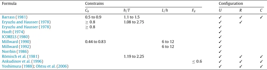
Barrass(1981) proposed a formulation based on model-scale experimental data and full-scale observations. His formula
Table 1
Empirical formulae constraints, adopted fromBriggs(2006).
Formula Constrains Configuration
Cb h/T L/h Fd U R C
Barrass(1981) 0.5 to 0.9 1.1 to 1.5 ✓ ✓ ✓
Eryuzlu and Hausser(1978) ≥0.8 1.08 to 2.75 ✓ ✓
Eryuzlu and Hausser(1978) ≥0.8 ✓
Hooft(1974) ✓
ICORELS(1980) ✓
Millward(1990) 0.44 to 0.83 6 to 12 ✓
Millward(1992) 6 to 12 ✓
Norrbin(1986) ✓
Römisch et al.(1981) 1.19 to 2.25 ✓ ✓ ✓
Ankudinov et al.(1996) ≤0.6 ✓ ✓ ✓
Yoshimura(1988);Ohtsu et al.(2006) ✓ ✓ ✓
* Trim, midship sinkage coefficient and squat.
other than the (Ankudinov et al., 1996), formulation, capable of calculating the stern squat as well as bow squat of a vessel,
which was developed based on model-scale experiments. Later,Millward(1990) proposed a solution, partly as a response
to the grounding of the ferry Herald of Free Enterprise (Millward, 1990). The formulas suggested in their paper are intended to be used as an aid in preliminary design calculations and were derived by analysing available experimental data. Later, in Millward(1992) the formulation was re-arranged to resemble the one proposed byTuck(1966). Following this,Eryuzlu et al. (1994) collected physical full-scale data and conducted model-scale tests on bulk carriers and cargo ships with bulbous bows in restricted and unrestricted waterways. Their investigation led to the development of a formula, which has one restriction less than the (Eryuzlu and Hausser, 1978) formulation. Namely, the validity of the formulae is not governed by the water depth.
To facilitate the comparison of the output from the different formulae detailed above, an in-house code was developed in this study. For this purpose, MATLAB was utilised due to the wealth of complex built-in, easy to understand and use
mathematical operators. The formulae coded, and their restrictions are shown inTable 1, whereUstands for horizontally
unrestricted waters,Rrepresents dredged/restricted channels andC– vertical walled canals:
2.2. Analytical methods
Interest in the field of shallow water hydrodynamics can be traced back to the famous paper by Michell(1898). In
his publication, he devised a thin-body method to predict the wave resistance of a ship moving in shallow water. The
fundamental assumption behind theMichell(1898) method is that the ship’s beam is small compared to its length. As
a consequence of this, the waves generated are also of small amplitude, which allows the linearisation of the free water surface. LaterJoukovski(1903) derived a similar formulation of the problem independently.
Havelock(1908) investigated the wave pattern created by the propagation of a point source in shallow water. His work led to the introduction of the non-dimensional depth Froude number (Fd)
Fd
=
V
√
gh (2)
WhereVis the vessel’s speed,gis the acceleration due to gravity (g
=
9.
81 m/
s) andhis the water depth. The depth Froudenumber can be thought of as the ratio of the ship’s speed to the maximum wave velocity in shallow water of depthh. The
well-known Kelvin wave pattern resulting from moving objects in water can be observed atFd
<
0.
57 (Tezdogan et al.,2015). As the ship’s velocity increases, the lateral wave lengths will increase untilFdbecomes1, which is called the critical
speed. The terms subcritical and supercritical speed are used for vessels propagating atFd
<
1 andFd>
1,
respectively. Ofgreater practical interest is the former scenario, namely when the depth Froude number is smaller than 1 (Beck et al., 1975). A critical paper, which can be said to have spiked the interest in shallow water hydrodynamics, was produced byKreitner (1934), who used a one-dimensional hydraulic theory to calculate ship squat. He showed that the equation for the flow velocity in a canal ceases to provide rational solutions as the critical speed is approached. This theoretical prediction made
has been extensively verified. It is well known from the work ofConstantine(1960), who investigated the relationship
between subcritical, critical and supercritical speed regimes and their effect on squat, that laterally restricted waterways have substantial effect on the dynamic squat of a vessel.
The wave-making resistance of ships in shallow seas and restricted waters was investigated by Inui (1954). The
abovementioned work showed that the wave-resistance of a ship in infinitely wide shallow water has a continuous character throughout the speed range. However, this does not hold for the first derivative of the resistance with respect to the velocity. On the other hand, the resistance itself is not a continuous function ofFdin the case of restricted shallow waters.Inui(1954)
Tuck(1966) reproduced Michell’s linearised Slender-body theory, using matched asymptotic expansions to solve for the hydrodynamic forces in shallow water. In his paper,Tuck(1966) explored the scenario where a ship is travelling in shallow waters of constant infinite width. He used the vertical forces and moments acting on the ship to successfully compute the sinkage and trim for sub- and supercritical speeds, and validated the results with model-scale experiments. The results
obtained showed good agreement with experimental results forFd
<
07 (Tuck, 1966). One of the main conclusions drawnin his study was that although the theory fails asFd
→
1 because the formulations used become singular, sinkage ispredominant in the subcritical range, while trim is the leading factor in the supercritical range. With regards to resistance,
the method developed byTuck(1966) predicts zero resistance in the subcritical range.Tuck(1966) postulates that if a
second order approximation is sought, non-zero resistance in the subcritical range would be achieved as a consequence of the introduction of additional finite-depth effects.
Later,Tuck(1967) investigated the effect of restricted channel width as well as depth on ship behaviour.Beck et al.(1975) expanded on the previously mentioned work to account for vessels in dredged canals (Fig. 2) with an infinite shallow water region of constant depth (h∞) extending on either side of the dredged section on the channel (of depthh0).
As reported inGourlay(2008), the theory described above is best suited for long, slender hulls such as high speed twin hull catamarans, frigates and destroyers. However, the Slender-Body theory has been successfully implemented on containership hulls whose beam (B) to length (L) ratio lies between 0.11 and 0.15. It is worth noting that the post-panamax containership (DTC) studied in this paper has a ratioB
/
L≈
0.
14, which falls within the restriction detailed above.Yasukawa(1993) presented a linearised method capable of calculating the wave-making resistance of a ship while taking into account the sinkage and trim based on double-body flow solutions. His approach was applied to the Wigley hull, and showed satisfactory predictions when compared to experimental data. Later, all linearised slender-body methods were
compiled and presented inGourlay(2008). He derived a general Fourier transform method to calculate the sinkage and trim
of a ship advancing in unrestricted shallow waters, canals and stepped channels as well as channels of arbitrary cross-section. The formulationsGourlay(2008) used in his paper focus exclusively on the subcritical range of motion. Later, he extended his modification of the Slender-body theory to calculate the sinkage and trim of a fast displacement catamaran propagating through horizontally unrestricted shallow water, which retains its validity for all speed regimes. Then,Gourlay(2008) went on to show how trim, resistance and sinkage are affected by a change in the spacing between the catamaran hulls. Although this method has not been verified against experimental results,Gourlay(2008) postulates that his theory could be used as a preliminary assessment of the sinkage a fast displacement catamaran will experience upon entering shallow waters.
Alderf et al.(2011) suggested the use of a finite element technique to assess the dynamic squat phenomenon. The model
developed in their paper was used to validate the stability model as an extension of the method proposed byJanssen and
Schijf(1953) by predicting the unstable squat positions for a vessel. Following this,Yao and Zou(2010) developed and tested their theory for a Series 60 hull (CB
=
0.
6). The approach used in their paper consists of a panel method, applied to calculatethe shallow water effects on a ship by discretising the hull, free and wall surfaces into panels on which Rankine sources of constant strength are distributed. The results obtained, which include sinkage, trim, resistance and wave patterns were calculated for sub- and supercritical speeds. The data was found to be in good agreement with experimental results.
Then,Alidadi and Calisal(2011) conducted a numerical study to predict the squat of the Wigley hull. A slender-body
theory approach was utilised to convert the three-dimensional ship problem into a series of 2-D cross sections distributed from the bow to the stern at equal intervals. They applied a boundary element method sequentially to each cross section to obtain the disturbance potential. By integrating the pressure over the hull, the forces acting on the hull were derived, which were then used to estimate the squat. A validation study was performed which compared the numerical results with those recorded from experiments at several speeds. The results between the two sets of data were agreeable.
Gourlay et al.(2015) performed a dynamic sinkage and trim comparison and analysis using the Slender-Body theory and Rankine-source method for different modern containership hull forms, including the DTC. The results were compared with experimental data for all case-studies. The key findings are that the Slender-Body theory provides good approximations when applied to wide canals or open water. However, it under predicts the sinkage in narrow canals. With regards to trim, Gourlay et al.(2015) showed that this parameter is accurately assessed for low speeds. The Rankine-source theory showed best performance when applied to the KCS, where the sinkage was similar to experimental results.
Finally,Feng et al.(2016) developed a Rankine source method which utilises the continuous distribution of source
panels along the free and seabed surfaces. In this way, no desingularisation was required, which facilitated the investigation performed byFeng et al.(2016) into the performance characteristics of a 2-D structure experiencing a forced oscillation, by removing any additional assumptions. To show the effect the proximity and topology of the seabed, several scenarios were investigated in their research article, including a deep water case-study, flat bottom shallow water, and various uneven
bottom topologies. One of the key findings made byFeng et al.(2016) was that the mean water depth is a key parameter
influencing the hydrodynamic performance of a body in shallow water.
2.2.1. Slender-Body theory
In this sub-section, the basis of the Slender-Body theory background is given. As a case-study the channels utilised by Beck et al.(1975) to derive their extension to the Slender-Body theory were used in this paper. The same notation used by Beck et al.(1975) is adopted to alleviate the nomenclature and results comparison. The basic concept is shown inFig. 2:
Fig. 2.Schematic drawing of a ship in dredged canal; a: Front view, b: Top view (Beck et al., 1975).
A crucial part of any physics modelling problem lies in the boundary conditions. For the dredged canal, the fluid velocity disturbance due to the presence of a vessel satisfies Laplace’s equation in both the interior and exterior regions. Ignoring the local behaviour of the fluid near the hull, the three-dimensional velocity potential can be reduced to 2-dimensions. Therefore, Laplace’s equation for the interior/exterior region takes the form of:
(
1
−
Fd2)
∂
2
ϕ
∂
x2+
∂
2ϕ
∂
y2=
0 (3)Where
ϕ
is used to denote the velocity potential. ForFd<
1, the solutions of Eq.(3)approximate an elliptical function; whileforFd
>
1 the solutions show a hyperbolic tendency. This paper will only deal with the cases where the solutions of Eq.(3)are elliptical, or in other words, the flow lies in the subcritical range. Then,Tuck(1966) goes on to describe the hull boundary condition, namely, the velocity normal to the hull is equal to zero:
∂ (
x+
ϕ)
∂
n=
0 (4)where
∂/∂
n is the derivative in the normal direction. Furthermore, the same boundary condition holds for the bottom of the channel∂ϕ∂z=
0.Utilising the results derived byTuck(1966), it follows from the mass conservation law that the velocity potential must satisfy the boundary condition, Eq.(5)(Gourlay, 2008):
∂ϕ
∂
y= ±
V
2h0
S′(x) aty
=
0i.
e.
at the hull (5)whereS(x) is the hull cross-sectional area at positionx, and prime is used to denote the derivativedSdx,h0is the interior water region depth, andVis the ship speed.
The second boundary condition contains two parts. Firstly, for a fluid extending infinitely in theydirection, the potential
ϕ
→
0 asy→ ±∞
forFd<
1. Secondly,ϕ
→
0 asx→ ±∞.
The bottom topography is described in the same terms as byBeck et al.(1975), to elaborate, the fluid extends throughout the region
−
h(
y) <
z<
0, whereh(y) can be described in terms of the interior region’s width as shown in Eq.(6):h(y)
{
ho
,
|
y|
< w/
2h∞
,
|
y|
> w/
2 (6)Eq.(6), implies that the location of the hull’s centreline and coordinate system coincide with the channel’s. Additionally, the
domain, occupied by the fluid can be separated in terms of two depth Froude numbersF∞
=
V/
√
gh∞which corresponds
to the exterior region andF0
=
V/
√
gh0, which corresponds to the interior region. In the paper byBeck et al.(1975), the flow in the interior region is always taken to be subcritical (F0
<
1). Therefore, the cases investigated are reduced to:1. The exterior region is subcritical (F∞
<
1) – the sub–sub case 2. The exterior region is supercritical (F∞>
1) – the sub–super caseIn both the studies ofBeck et al.(1975) andTuck(1966), the boundary condition, Eq.(5)is integrated by parts and the hull cross-sectional area is assumed to equal zero at the bow and stern. However, firstly, this assumption does not hold for modern transom ships (Gourlay, 2008). Secondly, for certain speeds, the flow cannot close immediately after the transom i.e. there is some flow separation in the stern section of the ship. Therefore,Gourlay(2008) proposed that the gradient of the sectional area should be taken as 0 ahead of and behind the vessel, instead. This allows for the boundary condition Eq.(5)to be used in its original form.Gourlay(2008) then employed the direct Fourier transform of the derivative of the cross-sectional area over the wetted length of the ship:
S′
(
k)
=
∫
∞−∞
According toGourlay(2008) this ensures the smooth detachment of the flow from the transom even at high speeds. Furthermore, in the abovementioned article, the author argues that the assumption of a ‘bang shut’ flow, i.e. no flow separation, behind the transom makes the derived theory less applicable to modern ships.
For stepped channels,Beck et al.(1975) proposed two methods for calculating the force and moment coefficients and
therefore the sinkage and trim. The first method uses the Fourier transform of the ship’s beam (b(k)) and the beam multiplied by the position (xb(k)). The alternative method utilises the convolution of the derivative of the cross-sectional area and the dimensionless parameterk(x)
,
mathematically defined as shown in Eq.(8):k
(
x)
=
⎡
⎣coth
π
xw
√
1−
F2 0−
1⎤
⎦
exp⎛
⎝
2θw
w
√
1−
F2 0⎞
⎠
(8) Whereθ
=
⎧
⎪
⎪
⎪
⎪
⎪
⎪
⎨
⎪
⎪
⎪
⎪
⎪
⎪
⎩
arctan⎛
⎝
h∞√
F2∞
−
1h0
√
1
−
F2 0⎞
⎠
forF∞<
1isgn(k)arctan
⎛
⎝
h∞√
1
−
F2 ∞h0
√
1
−
F2 0⎞
⎠
forF∞>
1(9)
wherei
=
√
−1 and
sgn(k) is the signum of the Fourier transform variablek.
Making use of the convolution method described byBeck et al.(1975), the resulting equations for the force and moment
coefficients (CfandCmrespectively):
Cm
=
∫
xb(x)−
∫
s′(ξ)
k(
x−
ξ)
dξ
dx2
w
L√
1
−
F02∫
b(
x)
x2dx(10)
Cf
=
∫
b
(
x)
∫
−s′(ξ)
k(
x−
ξ)
dξ
dx2
w
L√
1
−
F2 0∫
b(
x)
dx(11)
where
∫
−s′(ξ)
k(
x−
ξ)
dξ
dxis the convolution mentioned previously,∫
−is used to denote the Cauchy or principle value integral andξ
is the convolution variable.Eqs.(10)and(11), respectively, are used to calculate the sinkage and trim coefficients — Eqs.(12)and(13), respectively:
CS
=
Cf
−
α
Cm1
−
αβ
(12)Cϑ
=
Cm−
β
Cf1
−
αβ
(13)where the shape parameters
α
andβ
are defined in Eqs.(14)and (15):α
=
∫
xb
(
x)
dxL
∫
b(
x)
x2dx (14)β
=
L∫
b
(
x)
xdx∫
b
(
x)
x2dx (15)An interesting property that Eq.(14)to(15)exhibit is that they all vanish for a longitudinally (y-axis) symmetrical ship (Tuck, 1966). The explanation to this lies in the integration of the beam over the length, multiplied by the position function in Eqs.(14)and(15). For such a ship, the coefficients
α
andβ
must equal zero due to the integral in the numerator. Similarly, in E1.(10)integrating the beam over the length whenb(x) is a symmetrical curve yields zero.The expressions for the sinkage (Eq.(16)) and trim (Eq.(17)) proposed by (Tuck, 1966) retain their validity inBeck et al. (1975). To elaborate,
s
=
LCSF 2 0√
1
−
F2 0[m]
(16)t
=
CϑF 2 0√
1
−
F2 0The only change necessary to obtain a formulation for a ship advancing through a canal with vertical walls on either side or
h∞
/
h0=
1 and no infinite shallow water region, lies in the parameterθ
. As the ratio of the shallow water region to the deepwater region is part of the argument of the inverse tangent of
θ
, the parameterθ
→
0 for such a scenario. Therefore, nodifficulty arises in computing the coefficients of interest for different channel geometries. One of the key conclusions drawn byBeck et al.(1975) is that ash∞diminishes, the wave resistance increases. It is important to note that these results have yet to be validated. The current study incorporates several case-studies designed to investigate further into this prediction. An immediate inference drawn from this section is that most authors employ directly the Slender-Body theory, such as Gourlay et al.(2015),Gourlay(2007), (2008), (2009) andAlidadi and Calisal(2011). Alternatively, similar linearised methods are utilised in the literature to solve the problem of dynamic squat-induced sinkage, trim and resistance. One of the major shortcomings of these approaches is that the non-linear terms are neglected.Gourlay(2008) stated that these higher-order terms do not significantly affect the performance of slender bodies propagating in shallow waters. However, the behaviour of larger vessels that operate at relatively high speeds, such as containerships and car carriers, can be significantly influenced by this assumption.
2.3. Reynolds Averaged Navier–Stokes (RANS) based numerical techniques
In this section, the Computational Fluid Dynamics (CFD) contribution to the field of shallow water hydrodynamics is delineated. Unlike potential flow theories, CFD has not yet been used extensively to predict the sinkage, trim and resistance of
ships in shallow waters. For instance,Jachowski(2008) employed a commercially available RANS based numerical software
package to predict ship squat in shallow waters. He applied this technique to the KRISO Containership (KCS) model. In order to reduce the computational effort, all simulations performed in his paper were carried out in model scale. Additionally, a symmetry boundary condition was imposed due to the transverse symmetry of the flow around the hull (Jachowski, 2008). The results were compared to those calculated by empirical formulations and good agreement was found between the two methods.
Later,Prakash and Chandra(2013) performed a CFD analysis of a ship advancing through shallow waters using ANSYS
Fluent, a commercial RANS solver. Their paper consists of an investigation into the resistance of a river–sea ship at different speeds. The CFD based software was run in deep and shallow water, in model scale for different speeds, 5 of which in the subcritical, one critical and one in the supercritical range (Prakash and Chandra, 2013). The data obtained by CFD was
then compared to theHoltrop(1978) method for the deep water case. The method developed by Schlighting, an empirical
approach estimating the proportional increase in resistance when comparing deep and shallow water performance, was
used byPrakash and Chandra(2013) to validate the shallow water results (Lewis, 1988).
Wortley(2013) performed a CFD investigation of the sinkage and trim on the DTC containership in OpenFOAM, an alternative RANS solver.Wortley(2013) used two different software packages (Maxsurf and Michlet) to compare his results. Wortley(2013) reported that as a consequence of the insufficient resolution of the generated mesh in OpenFOAM, the wave resistance is overestimated. Furthermore, the sinkage and trim results obtained showed some disagreement with experimental results. As reported byTezdogan et al.(2016), provided that the CFD setup is refined, the results will agree well with the values obtained experimentally.
Castiglione et al.(2014) performed a numerical study on the interference effects of wave systems on a catamaran in shallow water. Their investigation was conducted using the CFDSHIP-Iowa RANS solver on the DELFT 372 catamaran model. As part of their study, two hull separation distances and three depth scenarios were computed for several speeds. Some of their key findings are that ship-generated waves and their interference change significantly and are more relevant in shallow, rather than deep water. Furthermore, shallow waters have a significant effect on the total resistance of a ship. To evaluate
the multi-hull performance of the catamaran,Castiglione et al.(2014) extended their research by incorporating mono-hull
case-studies as well.
Mucha and El-Moctar(2014) performed numerical analyses using potential flow and RANS methods and compared their results for sinkage, trim and resistance to available experimental data for the KCS model in shallow water. The resistance was predicted well by the RANS solver, while the potential flow method showed small deviations from experiments. One of the interesting findings from their study is that the frictional resistance of a ship is highly dependent on the underwater keel clearance (UKC). The results for sinkage and trim were also in good agreement with the available data. The RANS solver showed some deviation from the experimental data in the low speed range, which the authors attribute to reduced quality of the grid on the free surface. Finally, the authors concluded that there is a need for further systematic investigation into shallow water effects.
More recently,Tezdogan et al.(2016) investigated the performance and behaviour of the DTC in an asymmetric canal as
part of the Pre-Squat workshop initiated by the University of Duisburg–Essen (further information can be found in (Mucha et al., 2014)). Simulations were run for different even keel draughts and speeds to evaluate the effect of the asymmetric bottom
on the channel. To accomplish this,Tezdogan et al.(2016) employed CD-Adapco’s Star-CCM+ RANS solver and showed that
the results obtained in model scale are in good agreement with experimental results. Perhaps one of the most interesting findings was that a slightly increased large initial draught will magnify the effect of the shallow water region to a much greater extent than a significantly increased small initial draught (Tezdogan et al., 2016).
In this paper, the same vessel as the one used byTezdogan et al.(2016) is used and the numerical setup is the same
except the canal geometry. InTezdogan et al.(2016)’s study an asymmetric canal geometry was modelled as adopted from
Fig. 3.3D geometry of the DTC; modelled in Star-CCM+ (Tezdogan et al., 2016).
[image:10.544.39.514.333.427.2]Fig. 4.Hull sections of DTC (El-Moctar et al., 2012).
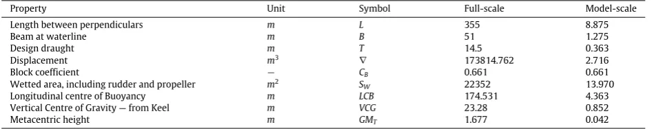
Table 2
DTC main particulars in full and model-scale (El-Moctar et al., 2012).
Property Unit Symbol Full-scale Model-scale
Length between perpendiculars m L 355 8.875
Beam at waterline m B 51 1.275
Design draught m T 14.5 0.363
Displacement m3 ∇ 173814.762 2.716
Block coefficient − CB 0.661 0.661
Wetted area, including rudder and propeller m2 S
W 22352 13.970
Longitudinal centre of Buoyancy m LCB 174.531 4.363 Vertical Centre of Gravity — from Keel m VCG 23.28 0.852
Metacentric height m GMT 1.677 0.042
3. Ship hull and channel geometry
As a case study for this paper, the DTC model was chosen for several reasons. Firstly, 3-D CAD (Computer-Aided Design) hull, propeller and rudder data are all readily available in the public domain. Secondly, as a response to the rapid developments of containership hull form design, the University of Duisburg–Essen developed this vessel for benchmarking purposes. The DTC was designed to be utilised as a model for numerous investigations, and various authors have made use of the DTC to conduct research (El-Moctar et al., 2012). A large number of experiments have been carried out in model scale
(1
:
40) and a wealth of data is available from different papers in both deep and shallow waters. Unfortunately, a steppedchannel model scale experiment is yet to be conducted, which is part of the reason why the present study incorporates this scenario.
For the reasons detailed above, the DTC is the perfect case-study for an investigation into the shallow water behaviour and performance of large vessels. A scale factor of 1:40 was chosen to match the experiments performed on this ship in other studies. A 3D model of the DTC as modelled in Star-CCM+ in shown inFig. 3and the hull sections are presented inFig. 4. As part of the initial conditions, an even-keel draught was set throughout the case-studies performed in this paper. The main particulars in full and model-scale are presented inTable 2.
Since the research idea behind this paper was to investigate the effect of the presence of a step in the channel, it is evident that this scenario will be focused upon. Furthermore, inBeck et al.(1975), great emphasis was placed on the height of the step in proportion to the overall depth. In this study, the abovementioned ratio (h∞
/
h0) was varied between 1 and 0 at threeequal intervals for each depth Froude number, as shown inTable 3. To increase the number of ways in which this study
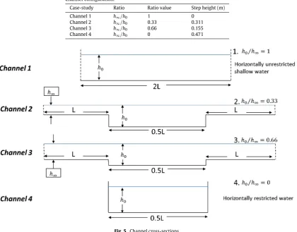
Table 3
Channel configuration.
Case-study Ratio Ratio value Step height (m) Channel 1 h∞/h0 1 0
Channel 2 h∞/h0 0.33 0.311
Channel 3 h∞/h0 0.66 0.155
Channel 4 h∞/h0 0 0.471
Fig. 5.Channel cross-sections.
The width of the inner region was chosen based on the results detailed byBeck et al.(1975). By reviewing the graphs
produced byBeck et al.(1975), it became evident that when the inner width to ship length ratio is equal to 0.5 the effect of the step is amplified. Therefore, this configuration was selected to investigate the influence of the depth discontinuity as this assumption is likely to produce the most palpable differences between configurations. The width of the domain in the research byBeck et al.(1975) is infinite, however, doing this in Star-CCM+, or in fact any CFD software is not possible, therefore, the transverse boundaries must be placed suitably, so that wave reflection does not influence the ship. According to the ITTC’s CFD guidelines, any boundary should be placed between 1 and 2 ship lengths away from the vessel (ITTC, 2011). To minimise the computational effort, the lateral boundaries were placed at a distance of 1 ship length away from the step on each side. This amounts to 1.25 ship lengths distance between the vessel’s centreline and the transverse boundaries on each side of the ship, as depicted inFig. 5.
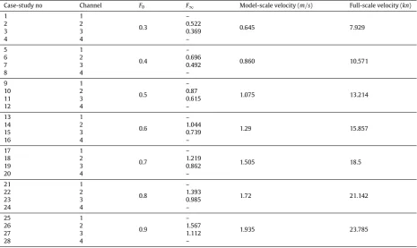
The case-studies detailed inTable 3are used in both the Slender-Body theory and CFD runs. To compare the performance
of these two different methods more accurately, as mentioned in the Introduction, each case-study is run for different speeds. Table 4shows in detail the model-scale and corresponding full-scale velocity for each run. Additionally, the channel cross-sections are shown inFig. 5.
4. Numerical modelling
Up to this point, this paper has been focused solely on the motivation and background of the theories and techniques used, and the logic behind the specific case-studies selected. In this section, the numerical modelling techniques will be discussed in detail. As stated previously, the numerical setup employed in this paper is similar to that explained in detail in Tezdogan et al.(2016).
4.1. Physics modelling
Table 4
Simulations cases applied to CFD.
Case-study no Channel F0 F∞ Model-scale velocity (m/s) Full-scale velocity (kn)
1 1
0.3
–
0.645 7.929
2 2 0.522
3 3 0.369
4 4 –
5 1
0.4
–
0.860 10.571
6 2 0.696
7 3 0.492
8 4 –
9 1
0.5
–
1.075 13.214
10 2 0.87
11 3 0.615
12 4 –
13 1
0.6
–
1.29 15.857
14 2 1.044
15 3 0.739
16 4 –
17 1
0.7
–
1.505 18.5
18 2 1.219
19 3 0.862
20 4 –
21 1
0.8
–
1.72 21.142
22 2 1.393
23 3 0.985
24 4 –
25 1
0.9
–
1.935 23.785
26 2 1.567
27 3 1.112
28 4 –
To model the turbulence in the fluid, a standardk
−
ε
model was employed with the all y+wall treatment, which has beenwidely used in similar studiesTezdogan et al.(2015,2016).Quérard et al.(2008) conducted a study in which the viscous
effects on ships were investigated. One of their key findings was that thek
−
ε
turbulence model is inexpensive in terms of CPU usage and can reduce the computational time significantly simultaneously providing solutions in good agreement with available data (ITTC, 2011;Quérard et al., 2008). The model selected here can be described as a two-equation model because it introduces two additional equations for the numerical software to solve, more specifically, one for the kinetic energy (k) and one for the dissipation (ε
). Moreover, as stated byCD-ADAPCO(2016), thek−
ε
model provides a good compromise betweenrobustness, computational cost and accuracy. As stated inTezdogan(2015) with a reference toCD-ADAPCO(2016) ‘‘the all
y+
wall treatment is a hybrid model, which provides a more realistic approach than the low-Re or the high Re treatments. To calculate shear stress, this well treatment uses blended wall laws, which present a buffer region that suitably blends the laminar and turbulent regions together. The result is similar to the low-Re y+
treatment as y+
→0 and similar to the high-Re
y+treatment for y+
values greater than 30’’.
To characterise the free surface, the volume of fluid (VOF) method was adopted to model and position the boundary between phases. This consists of a numerical technique for tracking and locating the fluid–fluid interface (CD-ADAPCO, 2016). The VOF model is defined in the Star-CCM+ user manual as ‘‘a simple multiphase model that is well suited to simulating flows of several immiscible fluids on numerical grids capable of resolving the interface between the mixture’s phases’’ (CD-ADAPCO, 2016). The suitability of this method for predicting the fine changes present in the free surface depends on the two immiscible fluids accounting for large structures in the domain, while their contact area should be relatively small (CD-ADAPCO, 2016). The concept of a flat wave is used to represent the movement of water particles relative to the ship hull in the context of this paper. The water surface is free to move, depending on the disturbance caused by the presence of the ship. An increased mesh resolution is imposed in the region where the free surface is expected to undergo sharp local gradients i.e. the formation of waves. The VOF model has shown excellent performance and high numerical efficiency in similar studies such as ones conducted byTezdogan et al.(2015,2016).
The convection terms in the Navier–Stokes equations are discretised using a second order upwind scheme. This was done to avoid the smearing of the free surface, which would likely happen if a lower order scheme had been adopted instead (CD-ADAPCO, 2016).
A segregated flow model was utilised to solve the governing Navier–Stokes equations in an uncoupled manner. To solve these equations, the Semi-Implicit Method for Pressure Linked Equations (SIMPLE) algorithm was utilised.
4.2. Time step selection
An important concept for convergence of numerically solved equations is the Convective Courant–Friedrichs–Lewy (CFL) number. The basic concept behind this dimensionless parameter is that if a flow is moving across a discrete spatial grid, its characteristics should be computed at each cell using a predetermined time step (∆t). This must be selected appropriately, so that the time it takes a fluid particle to move from one cell to the next, should be equal to or larger than the chosen value of∆t. Therefore, to ensure that all flow characteristics are captured within the generated grid of cellsCFLmust be
≤
1. Themathematical description of the Courant number is given in Eq.(18):
CFL
=
u∆t∆x
<
1 (18)whereuis the fluid velocity in m/s,∆tis the time step in seconds and∆xrepresents the length of the control volume or cell in metres. For the case-studies examined here, the Courant number was not kept constant. Instead, the time-step was modified to provide accurate solutions for the flow around the ship over the grid, which was not altered between the case-studies.
To control the time step, the Implicit Unsteady option of Star-CCM+ was selected. An alternative method for time-step selection, proposed by theITTC(2011) recommends that for resistance predictions,∆tis calculated as shown in Eq.(19):
∆t
=
0.
005∼
0.
01L/
V (19)whereLis the length in metres andVis the ship speed inm
/
s.In a similar study, where the DTC’s sinkage and resistance in shallow waters were analysed, a time-step convergence study was carried out, this suggested that∆tshould equal 0
.
0035L/
V, which is significantly lower than the formulation proposed by the ITTC (Tezdogan et al., 2016). Finally, the temporal discretisation was set as first order to discretise the time variant term in the governing Navier–Stokes equation. This model was selected because it offers a good compromise between accuracy and time required to run the simulation. Additionally, first order temporal discretisation has been shown to provide stable results and good convergence properties in similar studies suchTezdogan et al.(2016). Finally, one of the main advantages of employing first order time discretisation is that the Courant number must be lower than 1, rather than 0.5, which would be required had the alternative (2nd order) scheme been selected.4.3. Computational domain
In this section, justification behind the computational domain dimension selection is presented. Re-examining the
assumptions made byBeck et al.(1975), several guidelines for the domain arise: The width of the domain inBeck et al.
(1975) is infinite, however, doing this in Star-CCM+, or in fact in any CFD software is not possible, therefore, the transverse boundaries have been placed suitably.
CD-ADAPCO(2016), recommends that the velocity inlet of the computational domain for resistance prediction should be located at least one ship length upstream from the forward perpendicular, and the pressure outlet at least twice that distance downstream, from the respective perpendicular. The rationale behind this recommendation is that in rare occasions, wave reflection can occur, this can potentially render the results meaningless from a resistance analysis point of view. To conform
to these recommendations, the inlet boundary was set 1
.
22Lahead of the forward perpendicular and the pressure outlet2
.
23Ldownstream from the aft perpendicular (CD-Adapco, 2016, (Tezdogan et al., 2016)). To eliminate the possibility of a wave reflection from these boundaries, a VOF wave damping option was enforced, the length of which was set as to equal 1.
127L≈
10 m used in both longitudinal and transverse directions.There are several types of boundary conditions offered by the CFD software package. For the purposes of this study, only the enforced conditions will be discussed. The boundary in the positivex-direction was set as a velocity inlet, where the flat wave originates, and the negativex-direction was set as pressure outlet, which prevents backflow and fixes static pressure at the outlet. To allow the simulation to resemble real life towing tank experiments as close as possible, the domain
top was placed 1
.
127L≈
10 m away from the still waterline, where the Newman boundary condition was applied. Thisexpresses an assumption widely used in potential flow, which can also be useful in CFD modelling. Namely, the velocity normal to the surface is 0 as in Eq.(4). Next, the virtual towing tank bottom is set as a ‘wall’- this boundary condition, as
defined byPrabhakara and Deshpande(2004), expresses ‘‘that a moving fluid in contact with a solid body will not have any
velocity relative to the body at the contact surface’’. Employing the built-in (non-slip) function of Star-CCM+ describing this phenomenon, we have dealt with the domain bottom, sides and hull.
Thus, the computational domain is assembled and shown graphically inFig. 6for channel 2.
4.4. Mesh generation
Mesh generation was carried out in the facilities offered by Star-CCM+. This allows the user to make full use of the software’s automatic operations. Firstly, the region-based mesh generated is static in relation to the local coordinate system and therefore to the hull. Since the DTC’s appendages describe complex geometries (rudder, propeller), a high-quality
Fig. 6.Representative domain boundaries; Depicted: Channel 2 (h∞/h0=0.33).
Table 5
The number of cells, faces and vertices for each channel configuration generated by Star-CCM+.
Configuration Number of cells Number of faces Number of vertices
Channel 1 1971465 5894406 2085519
Channel 2 1915989 5721364 2030540
Channel 3 1920352 5734692 2035409
Channel 4 1833069 5465509 1935181
Fig. 7.Wall y+distribution on the hull surface.
The Prism Layer mesher was utilised to generate orthogonal prismatic cells next to the hull. This kind of layer mesh allows the software to resolve the near-wall flow accurately as well as capture the effects of flow separation (CD-ADAPCO, 2016). Resolving these parameters in sufficient detail depends on the flow velocity gradients normal to the wall, which are much steeper in the viscous turbulent boundary layer than would be implied by taking gradients from a coarse mesh.
Prism layer numbers were selected to ensure that the y+
value on the ship is maintained at a value lower than 1 in order to use the low-Re y+
treatment, as explained previously. This was also discussed in the Pre-Squat workshop byYahfoufi
and Deng(2014) as their results claim that accurate calculation of ship squat and resistance relies on the selection of the low-Re model. A graphical representation of the y+
wall function on the ship hull is given inFig. 7, where the average value is 0.00878.
A trimmed mesher option was selected, which is an efficient method of fabricating a high-quality grid for complex mesh
generation. The cells created by the trimmed mesher are predominantly hexahedral and have a minimal cell skewness.Fig.
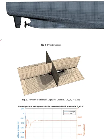
8shows the surface mesh on the hull with a focus on the stern of the ship. The computational mesh has areas refined in size around the hull, rudder and propeller as well as the areas where the free water surface is expected. The wake field behind the vessel also has a refined grid density to capture the complex flow properties (Fig. 9).
4.5. Convergence
Fig. 8.DTC stern mesh.
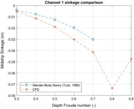
Fig. 9.3-D view of the mesh. Depicted: Channel 3 (h∞/h0=0.66).
Fig. 10.Convergence time–history of trim and sinkage for case-study No 16.
5. Results and discussion
[image:15.544.150.391.418.601.2]Fig. 11.In-house code output: Empirical formulae for channel 1.
Fig. 12.CFD and Slender-Body theory comparison for channel 1.
To begin with, perhaps the most interesting and most studied variable is analysed, namely, the squat. However, in order to obtain a full picture of the ship behaviour in shallow water, the trim the vessel experiences, considered an indispensable part in the overall ship assessment, is given for each case-study. The trim is given in radians, as the Slender-Body theory output uses this unit. The sinkage coefficients are also presented in this paper to facilitate future work.
5.1. Ship behaviour
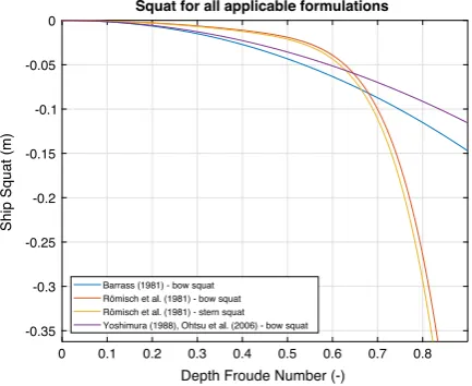
5.1.1. Channel 1
For this case-study, an attempt was made to approximate the scenario of a ship advancing through unrestricted shallow water. The theory developed byTuck(1966) describes this case-study, which has been shown to provide satisfactory results when compared to experimental data for low speeds. To perform the calculations, the Slenderflow code, which is validated in (Ha and Gourlay, in press) was used to provide results for all configurations investigated in order to ensure that the results are accurate. The empirical formulations for unrestricted waters were employed in the in-house code. The applicable formulae and the results computed using this method up toFd
=
0.
9 are shown inFig. 11.As discussed previously,Fig. 11highlights the main issue of this method of calculating ship squat. Namely, the results are highly divergent and disagree significantly, especially in the high-speed range.
[image:16.544.166.381.268.443.2]Fig. 13.Dynamic trim comparison for Channel 1; positive bow down.
Fig. 14.Wave patterns; Channel 1 atF0=a:0.3,b:0.5,c:0.7,d:0.9.
The results using the theory developed byTuck(1966) are continued up to and includingF0
=
0.
7 because non-linearand viscous effects become more important as we progress through the speed range. A slight underestimation of the CFD results can be observed throughout the velocities investigated, which is a consequence neglect of non-linear and viscous terms (Gourlay, 2008). As expected, the difference between the two sets of data gradually increases as the depth Froude number increases.
Finally, the trim comparison for this case-study is presented. The trim output from the in-house code developed for the empirical formulations is not shown as the results are several orders lower than the Slender-Body theory’s prediction or the CFD results.
Fig. 13reveals results, similar to those obtained byGourlay et al.(2015). To elaborate, the DTC trims by bow up toF0
=
0.
7, which is the upper limit investigated in the abovementioned work. The experimental results for the DTC both in a rectangular and non-rectangular canal, as inTezdogan et al.(2016), agree that the vessel squats by stern. The novel information presented here is that the DTC rapidly changes the trim mode to stern as the velocity increases pastF0=
0.
7.Fig. 15.In-house code output: Empirical formulae for channel 2.
Fig. 14reveals that atF0
=
0.
3 the disturbance caused by the DTC is hardly noteworthy, furthermore, the waves generated can scarcely be attributed to have been created by a moving ship, however, a depression around the hull is observed. As we increase the velocity, several noticeable changes occur. Firstly, the well-known Kelvin wake is developed. The bow wave begins to interact with the waves shed from the stern. This is more prominent inFig. 14bandc. Furthermore, the transverse length of the waves increases as we move up the velocity scale. Secondly, a depression in the water is observed originating from the bow and ending rather sharply as the stern is approached. The phenomenon termed hull speed, observed by William Froude, states that a ship can appear to be trapped between two wave crests at the Hull speed/displacement velocity in knots, mathematically defined in Eq.(20).Vh
=
1.
34√
L (20)
For the present case, after the units are converted intom
/
s,Vh=
2.
053 m/
s, which in terms of depth Froude number isF0
=
0.
955. Although the specific value has not been accounted for in the simulations carried out, the phenomenon hasalmost developed and is observable forF0
=
0.
9.InFig. 14a
,
bandca depression is present in the areas adjacent to the walls on either side ahead of the bow. This is most likely attributable to the fact that the DTC modifies the velocity, elevation and pressure in a region extending forward of the bow. This is most prominent in the low speed range, however, its origin is most clear in the high end ofF0.An important observation fromFig. 14is that the waves do not reflect from the side walls or interact with the ship
hull in any way. Therefore, the dimension selection detailed in the previous section accomplished its objectives, namely, to approximate an infinitely wide shallow water region for this configuration.
Finally, the change in the wave patterns observed atF0
≥
0.
7 coincides with the rapid change in the trend of the sinkage and trim values as shown inFig. 12andFig. 13, respectively. As alluded to previously, a consensus exists when it comes to high speeds in shallow waters. Namely, the trim increases, while the sinkage decreases in relative importance. This statement is valid for the present case-studies.5.1.2. Channel 2
In this section, the second case-study results are presented. For the two dredged channels (channel 2-h∞
/
h0=
0.
33 and channel 3-h∞/
h0=
0.
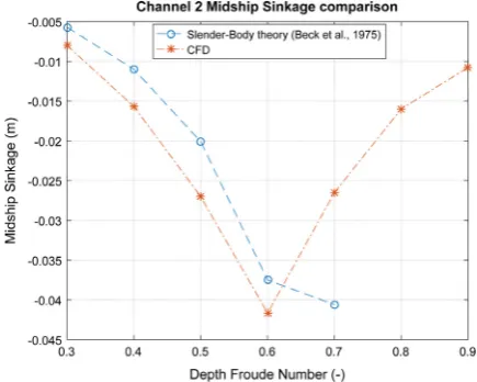
66), only the empirical formulations which retain their validity for restricted configurations are applicable, as shown inFig. 15. The first inference made here is regarding the results computed via the (Römisch et al., 1981) formulae for stern and bow squat. Due to the power at which the velocity is raised (34), the values become highly divergent towards the end of the velocity range.The results computed via the Slender-Body theory for dredged channels and CFD are shown inFig. 16.
The results for this case-study are of particular interest due to the exterior flow becoming supercritical (F∞
→
1)asF0
→
0.
6. As before, the Slender-Body theory under predicts the CFD values throughout the majority of the rangeinvestigated due to the absence of non-linear and viscous terms in the theory. Similarly to the first case-study, the sinkage
decreases in magnitude as the critical range is approached, as forecasted byTuck(1966). In the present case-study, the
sinkage curve slope is rapidly inverted afterF0
=
0.
6. Comparing the trend exhibited by the sinkage values for channel 1 (Fig. 12) and the current case-study reveals the significant influence of the exterior dredged section.Fig. 16.CFD and Slender-Body theory comparison for channel 2.
Fig. 17.Dynamic trim comparison for Channel 2; positive bow down.
exterior flow becoming supercritical at approximatelyF0
=
0.
6. The trim experienced by the DTC in the low speed rangeis significantly smaller, and changes from trim by bow to by stern much earlier than previously observed. Next, the wave elevation distributions in the computational domain are presented inFig. 18.
InFig. 18, dramatic changes are observed when compared to the channel 1 plot of wave elevation distributions (Fig. 14). Firstly, the step has a clear effect on the vertical displacement of the free surface. InFig. 18the water displacement is significantly influenced so that the position of the step is clearly visible around and ahead of the bow from the disturbance caused. Furthermore, the wave pattern behind the vessel is significantly modified by the depth discontinuity. As shown in Eq. (2), the wave velocity is expressed byC
=
√
gh, wherehis the water depth andgis the acceleration due to gravity. Now, in the interior region, this expression attains a higher value (C0=
√
gh0) when compared to the exterior region (C∞
=
√
[image:19.544.162.379.266.444.2]Fig. 18.Wave patterns; Channel 2 atF0=a:0.3,b:0.5,c:0.7,d:0.9.
pitch displacement seems to be more important in the higher end of the speeds investigated for channel 2 when compared to channel 1.
Finally, it is likely that the large displacement of the free surface under the computational domain has resulted in numerical inaccuracies. To elaborate, an insufficient section of the water surface has been modelled where the fluid interface is located beneath the computational domain. One way to tackle this would be imposing an overset mesh. In effect, this ‘overlapping’ or ‘Chimera’ mesh envelopes the moving body (in the current scenario, the DTC) into a finer resolution box-shaped mesh. The local coordinate system is then linked to this new region, rather than the entire computational domain, therefore, the influence of the large pitch displacement can be limited. However, in cases such as the one examined here, where the body is close to the boundaries of the domain, the overset mesh region is likely to collide with the towing tank bottom, thus rendering a similar result or causing the simulation to fail.
5.1.3. Channel 3
In this section, a case-study with a relatively deep exterior shallow water region (h∞
/
h0=
0.
66) is presented. The applicable empirical formulae retaining their validity are the same as those shown in the previous section for channel 2, asshown inFig. 19. As before, an upper limit equal to the ship’s draught was set for the results computed via the (Römisch
et al., 1981) formula. As shown inFigs. 19and15, the results are not highly affected by the change in the exterior shallow water region’s depth according to the empirical formulae.
The midship sinkage comparison between the Slender-Body theory and CFD is shown inFig. 20. The theory ofBeck et
al.(1975) behaves in a similar fashion as was the case for channel 2. The CFD results are underpredicted throughout the
investigated velocity range, however, the difference seems to increase more in proportion as we progress towards the critical speed. This is likely since viscous and non-linear terms attain a higher relative importance than was the case for channel 2. The typical decrease in sinkage magnitude is observed as the velocity in increased.
The trim comparison between CFD and the Slender-Body theory, for channel 3 is shown inFig. 21.
A similar trend is observed as for the previous case study inFig. 21. Namely, the trim distribution increases in magnitude as the velocity is increased. Furthermore, the two sets of data agree remarkably well in the low speed range. As the exterior flow becomes critical (atF0
≈
0.
8), the trim begins to exhibit significant increase in amplitude. More specifically, it changes from by bow to by stern rather sharply and attains a large amplitude towards the high end of speeds investigated. In alllikelihood, beyondF0
=
0.
7, nonlinear and hence viscous effects dominate the behaviour and performance of the DTC.Fig. 19.In-house code output: Empirical formulae for channel 3.
Fig. 20.CFD and Slender-Body theory comparison for channel 3.
[image:21.544.162.379.486.666.2]