A pipe organ-inspired ultrasonic transducer

A Pipe Organ-Inspired Ultrasonic Transducer

A

J. W

& A

J. M

*School of Science and Sport,

University of the West of Scotland,

Paisley,

PA1 2BE,

United Kingdom

† Department of Mathematics and Statistics,

University of Strathclyde,

Glasgow,

G1 1XH,

United Kingdom

Abstract

This article considers a number of backplate designs for the bandwidth improvement of electrostatic ultrasonic transducers in both transmission and reception modes. Motivated by the design of pipe organs, transducers with backplates which incorporate a number of acoustically resonating conduits are modelled using a transmission line mathematical model which describes the displacement of the electrostatic membrane. The model illustrates that by increasing the number and varying the length of these conduits, the trans-mission voltage response and the reception force response can be improved over the traditional design by around 50% and 35%, respectively. ultra-sound; transducer; pipe organ; electrostatic

1 INTRODUCTION 2

1

Introduction

Ultrasound is employed in a wide variety of applications including medical imag-ing, non-destructive evaluation, industrial cleaning and SONAR (see Ladabaum et al. (1998) and Leighton (2007)). Ultrasound is used by many animals such as bats (see Amichai et al. (2015)), dolphins (see Au (1993)) and insects (see Barber & Kawakara (2013)) using highly advanced, nonlinear generation and de-tection facilities. In the absence of these facilities, humans rely on electrostatic and piezoelectric transducers for the generation and detection of ultrasonic waves (see Mantheyet al.(1992) and Warring & Gibilisco (1985)).

Electrostatic transducers consist of a thin dielectric membrane stretched across a conducting backplate. The backplate is often grooved in order to trap air beneath the membrane and reduce its rigidity (see Schindelet al.(1995)). Recently, ultra-sonic transducers with acoustic amplifying conduits emanating from a machined cavity in the backplate have been designed, modelled and tested (see Campbell et al. (2006), Walker et al. (2008), Walker & Mulholland (2010) and Walker & Mulholland (2016)). These investigations have shown an improvement on two key factors, namely the gain of the transmission voltage response (TVR) and the reception force response (RFR). However, many applications require not only a high TVR/RFR gain, but a large bandwidth, so that the device can operate over a large frequency range. This would enable these devices to transmit and receive signals with a rich frequency content, such as chirps, as used in the animal world (see Maurello et al.(2000)). It would also improve the axial resolution of these devices as narrower impulses could be generated in the time domain. With this in mind, it is imperative that backplates can be designed which maximise the opera-tional bandwidth of electrostatic transducers.

This article considers a range of designs using an automatic sampling proce-dure, a self-similar design with a geometric progression of length scales and some designs inspired by the key features of pipe organs. A mathematical model is con-structed which outputs the operational bandwidths of the proposed transducers and these are then compared against similar outputs for a standard electrostatic transducer design. We find that all designs which incorporate acoustic ampli-fying conduits increase the operational bandwidth in the transmission mode and 95% of the designs increase the operational bandwidth in the reception mode. We also find that while the pipe organ-inspired transducer out-performs the standard transducer, it is in-turn outperformed by a self-similar design with a geometric progression of length scales.

2 PIPE ORGANS 3

2

Pipe Organs

Pipe organs produce sound by driving pressurised air through a series of pipes via a keyboard. The design of the individual pipes affects the sound produced, with design aspects consisting of length, radii, thickness, construction material, shape, scale (ratio of diameter to length) and presence or absence of a reed (see Bonavia-Hunt (1947), Barnes (1952), Fletcher (1977), Helmholtz (1895), Hop-kins (1855), McVicker (1987) and Rucz (2015)). A rank of pipes covers each note on a standard keyboard (normally 61 pipes) and pipe organs generally have a certain amount of ranks (normally at least ten, but often with hundreds). Each rank has a certain type of pipe and by pulling a certain ‘stop’, the organist can con-trol from which rank of pipes they will hear the key presses. In each rank, the stop refers to the largest pipe in the rank, each successive pipe is then slightly shorter to account for each of the 61 keys on a standard keyboard. For example, the pipe organ situated at the University of Strathclyde’s Barony Hall (see Figure 1) has 41 stops, ranging from 16-foot metal Quintadena pipes, through 8-foot metal Dulcian pipes with oak boots, to 4-foot oak Blockfl¨ote pipes with the smallest rank being 2-foot metal Cornet pipes (The University of Strathclyde (2016)). Furthermore, the diameter of each pipe is scaled according to normalmensur. That is, the diam-eter of each pipe is halved every 17 pipes (depending on type of pipe) where, in this case, 17 is the halving number. In normalmensur, the center C is generally an 8-foot stop with diameter 155.5 cm and every other pipe in the rank is calculated with respect to this design. The scaling of the pipes follows the 1 :√48 ratio, or

d_n= d1

2nh−−11

, (2.1)

wherednis the diameter of thenthpipe andhis the halving number. Each pipe will

relate to one specific note on the musical scale and sometimes length-adjusting collars are required in order to get the produced sound to the exact required fre-quency (see Joneset al.(1941), Nolle (1979) and Fletcher & Rossing (1991)).

2 PIPE ORGANS 4

Figure 1: The pipe organ situated at the University of Strathclyde’s Barony Hall.

3 MATHEMATICAL MODEL 5

3

Mathematical Model

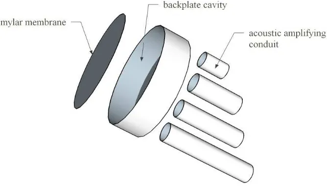
The mathematical model used in this article is a transmission line (1D in space) model introduced by Walker & Mulholland (2010) and discussed further by Walker & Mulholland (2016). The model outputs the transmission voltage response (TVR) and the reception force response (RFR) of the ultrasonic transducer, from which the bandwidths are calculated and compared against the standard transducer de-sign. As mentioned, standard electrostatic transducers operate by electrically ex-citing a stretch mylar membrane over a conducting backplate. The novel design considered in this approach uses acoustic amplifying conduits emanating from an air-filled cavity in the backplate. A simplified exploded sketch of the design is shown in Figure 2.

Figure 2: A simplified exploded schematic of the cavity/conduit de-sign. Note that tens or hundreds of acoustic amplifying conduits could emanate from the cavity.

3 MATHEMATICAL MODEL 6

3.1

Backplate Impedance Model

A single acoustic amplifying conduit, consisting of an open cylinder with radius rp and length lp, is first considered. Assuming that this conduit represents a

straight, open cylindrical pipe of a pipe organ, where the wavelength of the sound is large in comparison to the radius of the conduit (that is,c/f r_p, validated in Tables 1 and 2), the mechanical radiation impedance, Rp, at the open end of the

conduit is given by (see (Kinsleret al., 2000, p.272-274))

Rp=cρaγ

1 4(klp)

2_+0.6jkl p

, (3.1)

where f is the frequency of sound, cis the speed of sound, ρa is the density of

air, γ =πr2_p is the cross-sectional area of the conduit, k= (1+αj)ω/c is the

wavenumber of the sound, withα a nondimensional attenuation coefficient,ω the

angular frequency and j=√−1. Consequently, the specific acoustic impedance of the conduit at the conduit/cavity interface,Z_sp, is given by (see Walker & Mul-holland (2010))

Z_sp= cρa(Rp/(cρaγ) + jtan(klp))

1+j(R_p/(cρaγ))tan(klp)

. (3.2)

As mentioned, the backplate shall be designed with that of a pipe organ in mind. That is, the backplate shall incorporate an array of conduits. Consequently, each conduit’s impedance must be combined to form a lumped acoustic impedance which can then be used to calculate the impedance of the backplate. Defining Zp[i,j]as the acoustic impedance of the conduit in theith row and jth column of the array of conduits, the lumped acoustic impedance of the conduits is given by (see (Kinsleret al., 2000, p.288-291))

Zp=

1

∑N_j=1∑nj_i=11/Zp[i,j]

, (3.3)

wherenj is the number of conduits in row jand N is the number of rows in the

conduit array. Consequently, the specific acoustic impedance in the cavity,Z_sc, can be found via

Zc_s = cρa(Zp/(cρaSc) + jtan(klc))

1+ j(Z_p/(cρaSc))tan(klc)

, (3.4)

3 MATHEMATICAL MODEL 7

3.2

Transmission Line Model of Membrane Displacement

As shown by Walker & Mulholland (2016), the displacement of the membrane can be modelled via a pipe-driver system, a membrane model or a plate model. As each of these model produces similar results, we shall use the pipe-driver system detailed by Kinsler et al. (2000). Here, the membrane is assumed to act like a damped harmonic oscillator, which is excited by an external force f(t). Following the analysis by Walkeret al.(2008), Walker & Mulholland (2010) and Walker & Mulholland (2016), the dynamic equation for the membrane displacement ξ is

given by

d_mρsξ¨+

R_v S_m+Z

l s+

S_c S_mZ

c s ˙ ξ+

S_cZ_mc S_mV_c−

ε0V_dc2

d3 e

ξ = f(t), (3.5)

whered_mis the thickness of the membrane,ρsis the density of the membrane,Rv

is a damping constant, Sm is the surface area of the membrane, Zsl is the specific

acoustic impedance of the fluid load,Z_mc is the mechanical impedance of the cav-ity, V_c is the volume of the cavity, ε0 is the permittivity of free space,Vdc is the

direct current voltage, de is the distance between the electrodes and an overhead

dot represents the time derivative. The external force, which combines the voltage driving force applied to the membrane and any incoming pressure wave P(t), is given by

f(t) = ε0VdcVac(t)

d2 e

+P(t), (3.6)

whereV_ac(t)is the a.c. voltage. Clearly,V_ac(t) =0 in reception mode andP(t) =0 in transmission mode. Taking the Fourier transform (see Wright (2005)) of the differential equation (3.5) gives

Ξ(ω) = 1

jωZ_sm(ω)

¯

f(ω), (3.7)

whereΞ(ω)is the displacement of the membrane in the frequency domain,

¯

f(ω) =ε0VdcV¯ac(ω)/de2+P¯(ω), with ¯Vac(ω) the alternating current voltage in

the frequency domain, ¯P(ω)the incoming pressure wave in the frequency domain

and

Z_sm(ω) = jdmρs+

R_v

Sm

+Z_sl+ Sc

Sm

Z_sc

− j

ω

S_cZ_mc

SmVc

−ε0V

2 dc

d_e3

, (3.8)

is the specific acoustic impedance of the combined membrane/load system. Con-sequently, the velocity of the membrane in the frequency domain is

˙

Ξ(ω) = 1

Zm s (ω)

¯

3 MATHEMATICAL MODEL 8

The velocity of the mylar membrane’s deflections can then be used to compute the electrical impedance and hence the transmission and reception sensitivities of the device, as seen in the following section.

3.3

Electrical Impedance, Transmission and Reception

Sensi-tivities of the Device

A transducer converting electrical and mechanical energy forms a two-port net-work that relates electrical quantities at one port to mechanical quantities at the other (see Kinsleret al.(2000)). The canonical equations which describe this are given by

¯

V_ac=Z_EBI+TΞ˙, F =T I+ZmoΞ˙, (3.10)

whereI is the current at the electrical inputs,F is the force on/from the radiating surface, Z_EB is the blocked electrical impedance ( ˙Ξ=0), Zmo is the open-circuit

mechanical impedance (I=0) and T is the transduction coefficient (mechanical ↔electrical). In the short circuit case ¯V_ac=0 it can be shown

F ˙

Ξ =

Zmo−

T2 Z_EB

=Zm, (3.11)

whereZ_mis the mechanical impedance of the transducer. Hence equations (3.10) can be rewritten as

¯

Vac=ZEBI+βZEBΞ˙, F=βZEBI+ZmΞ˙, (3.12)

where the transformation factorβ is given byβ =T/ZEB. When the source

volt-age is of the form V_ac(t) =V_aceiωt_{, then by Caronti et al. (2002), Kinsler et al.}

(2000) and Walker & Mulholland (2010)

V_ac=

1 G+iωC0

I+ Vdc

iωx_dc ˙

Ξ, (3.13)

where G is the static conductance caused by electrical losses in the device, C₀ is the value of the capacitanceC at ˙Ψ=0 and xdc is the deflection of the

mem-brane caused by the d.c. voltage. Hence, comparing with equations (3.10) the transformation factor β can be found (see Walker & Mulholland (2010)) and,

consequently, the blocked electrical impedance is given by

Z_EB= 1

G+iωC0

4 COMPARISON OF TRANSDUCER DESIGNS 9

whereC₀=ε0Sm/(dm/εr+L+xdc), withεr the relative permitivitty of the

mem-brane andLthe distance between electrode and membrane.

In transmission mode, a voltage ¯V_ac is applied that results in a membrane ve-locity ˙Ξand hence a forceFbeing produced, whereF=−ZmΞ˙. The transmission

sensitivity, or transmission voltage response (TVR), is defined as the ratio of the transmitted pressure to the driving voltage (see Caronti et al. (2002)) and after some some algebraic manipulation, it can be shown that (see Walker & Mulhol-land (2010))

TVR= −ωVdcC0+iGVdc ωxdc 1+SmZms /Zl

. (3.15)

This can now be evaluated using the specific acoustic impedance of the combined membrane/load system, given in (3.8), and the acoustic impedance of the load, given by Kinsleret al.(2000) as

Zl= ρac

S_m



1−

J₁

2kpS_m/π

kpS_m/π

+j H₁

2kpS_m/π

kpS_m/π 

, (3.16)

where J_n is the Bessel function of the first kind of order n andH_n is the Struve function of ordern.

The reception sensitivity is defined as the ratio of the open-circuit (I =0) output voltage to the force on the membrane (see Carontiet al.(2002)). That is, the reception force response (RFR) is given by RFR=V¯ac/(PoSm), where Po is

the pressure produced at the membrane load. SettingI=0 (for the open-circuit) in equations (3.10) gives

¯

Vac=TΞ˙, F =ZmoΞ˙. (3.17)

Since F =P_oS_m then ˙Ξ=PoSm/Zmo and so it can be shown that (see Walker &

Mulholland (2010))

RFR= ΞZEB

S_mZm

s +T2/ZEB

. (3.18)

This can be evaluated via equation (3.14) and the specific acoustic impedance of the combined membrane/load system, given in (3.8), which is highly dependent on the design of the transducer’s backplate.

4

Comparison of Transducer Designs

4 COMPARISON OF TRANSDUCER DESIGNS 10

specific designs as described below. In order to successfully compare the devices, the material and other parameter values must be considered. Initial endeavours in manufacturing a variety of backplates have taken place by Hamid (2013) and Campbellet al.(2006) and form the basis for the backplate design parameter val-ues given in Table 1. The (constant) radius of the conduit(s) is chosen so that up to 100 conduits could fit in the backplate (see The Engineering Toolbox (2016)). Additional design and material parameter values are given in Table 2.

Design parameter Symbol Magnitude Dimensions

Thickness of membrane d_m 8 µm

Length of cavity lc 35 µm

Radius of conduit(s) r_p 26 µm

Surface area of membrane S_m π×3002 µm2

Surface area of cavity S_c π×3002 µm2

Table 1: Standard design values of the backplate.

Design Parameter Symbol Magnitude Dimensions

Speed of Sound in Air c 343 m/s

Damping Coefficient R_v 100 kg/m s

Applied Voltage V_ac 200 V

d.c. Voltage V_dc 200 V

d.c. Deflection on membrane x_dc 60 nm

Attenuation Coefficient α 0.001

-Permittivity of Free Space ε0 8.85×10−12 F/m

Membrane Dielectric Constant εr 5

-Density of Air in Resonator ρa 1.2 kg/m3

Density of Mylar Membrane ρs 1420 kg/m3

Table 2: Parameter and design values of the transducer.

We note here a justification of the lumped impedance model, described in Sec-tion 3, with the backplate design parameter values, given in Table 1. EquaSec-tion (3.1) refers to the mechanical radiation impedance of each conduit. These conduits have a radius which is 26µm and this is many times smaller than the acoustic

wave-length in air at 400 kHz, which is of the order of millimeters. The frequency range of interest is from 100 kHz to 400 kHz and so the corresponding wavelength range is from 800µm to 3430µm. The wavelength is also much greater than the radius

of the backplate which sits at 300µm. Hence, the requirement that c/f rp,

4 COMPARISON OF TRANSDUCER DESIGNS 11

In order to compare the different designs, the operational bandwidth of each device’s TVR and RFR is considered. For the TVR comparison, we let Abe the set of frequencies f for which the TVR sensitivity lies above a certain threshold. That is,

A={[ai,bi],i=1, . . . ,N: TV R(f)>τ,∀f ∈[ai,bi]}. (4.1)

Here, the thresholdτ is defined to be−3 dB below the maximum TVR sensitivity

of the standard design, which is described fully below. The operational bandwidth of the TVR of each device is then defined as

BW = N

∑

(b_i−a_i). (4.2)

The comparison of the RFR for each device follows a similar approach. Of course, care must be taken here as the set Acould consist of a series of disjoint intervals and so the frequency range over which the device is to be operated within could contain some bandgaps. Nevertheless, it is important to illustrate the total range of frequencies for which these new proposed devices outperform the standard devices. Note also that no damping has been included in either model and so, when introduced, this will serve to smooth out the peaks in these plots.

4.1

Standard Design

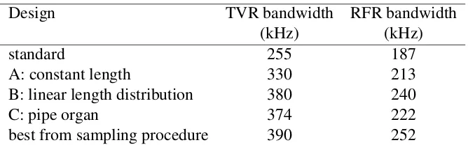
The standard cavity-only design has a closed cavity with length and surface area specified in Table 1. The bandwidth at the half-power point (−3 dB) is calculated for each metric and found to be around 255 kHz and 187 kHz for the TVR and RFR, respectively. It is these values which the new designs will be compared against, as illustrated in Equations (4.1) and (4.2). Plots of the TVR and RFR for the standard design can be found in Figures 4 (dotted line) and 6 (dash-dot-dot line).

4.2

Sampled Designs

Five thousand different designs were sampled where each design is given a ran-dom number of conduits between 10 and 100. Each conduit has the same radius, stipulated in Table 1 but each conduit length was randomly chosen from a lin-ear distribution with lp∈[0.4 mm,1.4 mm]. The TVR and RFR bandwidths are

4 COMPARISON OF TRANSDUCER DESIGNS 12

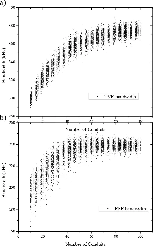
The ten devices with the smallest bandwidths have a number of conduits from the set {10,11,12}in transmission mode and from {10,11,12,14} in reception mode. In fact, changing the sampling procedure to choose from between 1-100 conduits means that the smallest ten bandwidths come from designs with a single figure number of conduits. Nevertheless, we see from Figure 3 that in transmission mode, every design outperforms the standard cavity-only device by at least 34 kHz (10 pipes) and up to 134 kHz (79 pipes) - an improvement of around 53%. In re-ception mode, we find that 95% of the sampled designs outperform the standard design, by 65 kHz in the best case (61 pipes), which equates to an improvement of around 35%. The worst case (10 pipes) shows a reduction in the bandwidth of 3 kHz, which equates to a reduction in bandwidth by around 5%. The TVR and RFR of the devices with the largest and smallest bandwidths are plotted in Fig-ure 4 alongside the cavity-only standard design, for comparison. We see that the inclusion of many pipes with different lengths creates multiple resonances which leads to a broader spectrum.

A frequency plot of the lengths of the conduits in the best and worst transmis-sion designs is presented in Figure 5. We note that there is no definite pattern as to what design produces the largest bandwidth for the TVR or RFR. The only clear metric which significantly changes the bandwidth is the number of pipes. How-ever, it could be postulated that a distribution of pipes where a linear progression of lengths is employed could fit much of the profile for best TVR and RFR seen in Fig. 5.

With this in mind, we now consider a number of specific designs which are made in order to test the hypothesis that the radii of the pipes are of no real signifi-cance, and that a linear array of pipe lengths should produce the largest bandwidth due to the coupling effect of resonances at many different frequencies.

4.3

Specific Designs

Three further designs are considered: designAinvolves 100 conduits all of con-stant length but with radii chosen according to the normalmensur equation (2.1) and designBinvolves 100 conduits all of constant radii, but with a linear progres-sion of pipe lengths in the rangelp∈[0.4 mm,1.4 mm]. DesignC, inspired by the

pipe organ, was detailed in Section 2: there are five ranks of 61 conduits each, the conduits in each rank have a length that is half of the previous rank, with the first rank designed to resonate at 100 kHz. Furthermore, the radius of the conduit in each rank is scaled according to the normalmensur scaling equation (2.1).

4 COMPARISON OF TRANSDUCER DESIGNS 13

0 20 40 60 80 100

280 300 320 340 360 380 400 TVR bandwidth B a n d w id th ( k H z )

Number of Conduits

(a)

0 20 40 60 80 100

160 180 200 220 240 260 RFR bandwidth B a n d w id th ( k H z )

Number of Conduits

(b)

Figure 3: TVR (a) and RFR (b) bandwidths of 5000 samples of device where the number of pipes is randomly sampled between 10 and 100. Each pipe has a length between 0.4 mm and 1.4 mm and a radius of 26µm. We see that, in general, more

pipes produce an improved bandwidth.

standard design with no conduits but illustrates that variety in conduit length is required.

4 COMPARISON OF TRANSDUCER DESIGNS 14

100 150 200 250 300 350 400

-60 -50 -40 -30 -20 -10 0

TVR (dB)

frequency (kHz)

best TVR from sample worst TVR from sample standard design

(a)

100 150 200 250 300 350 400

-60 -50 -40 -30 -20 -10 0

RFR (dB)

frequency (kHz)

best RFR from sample worst RFR from sample standard design

(b)

Figure 4: Best (solid) and worst (dashed) TVR (a) and RFR (b) against frequency from 5000 transducer design samples. Also included are outputs from the standard design (dotted).

an appropriate choice of conduit number and dimensions, the backplate can be designed to boost the device’s operating bandwidth at a desired frequency range.

4 COMPARISON OF TRANSDUCER DESIGNS 15

Figure 5: Frequency plots of the best TVR (dotted), best RFR (dash-dot), worst TVR (dash) and worst RFR (solid) devices from a sample of 5000 where the number of pipes is randomly sampled between 10 and 100. Each pipe has a length between 0.4 mm and 1.4 mm and a radius of 26µm. The best design has 79 pipes

in the transmission mode and 61 in the reception mode. The worst has 10 pipes in the transmission mode and 10 in the reception mode. No obvious pattern can be seen in the best case histogram other than more pipes generally equates to a better output.

distribution of pipes, nor the best randomly sampled device.

5 COMMENTS AND CONCLUSIONS 16

Design TVR bandwidth RFR bandwidth

(kHz) (kHz)

standard 255 187

A: constant length 330 213

B: linear length distribution 380 240

C: pipe organ 374 222

best from sampling procedure 390 252

Table 3: TVR and RFR bandwidths for standard design, specific designs and best design from the sampling procedure.

5

Comments and Conclusions

This article considers a number of backplate designs for the bandwidth improve-ment of electrostatic ultrasonic transducers. Based on the design of pipe organs, a transducer backplate design is presented and the transducer’s transmission volt-age response and reception force response are investigated. The output metrics are compared with that of a standard backplate design, some randomly sampled de-signs and some specific dede-signs which incorporate acoustic amplifying conduits. We find that all designs which incorporate acoustic amplifying conduits emanating from the backplate have a greater transmission mode bandwidth than that of the cavity-only device. This is due to the resonant behaviour of the conduits, which amplify the signal at specific frequencies. By incorporating conduits which have a range of length scales, the individual resonances couple to provide a signal with a wide bandwidth with up to a 50% improvement on the cavity-only device. It is seen that, in general, the more conduits there are (of varying lengths), the greater the bandwidth of the output signal. Specific designs for specific outputs (be that large gain at a particular frequency, or large bandwidth over a particular frequency range) can be modelled. The reception mode analysis shows a similar improve-ment over the standard design. Improveimprove-ments can be found of up to around 30% and, the designs can be tuned to operate over a specific bandwidth range.

5 COMMENTS AND CONCLUSIONS 17

100 150 200 250 300 350 400

-60 -50 -40 -30 -20 -10 0

TVR (dB)

frequency (kHz) best from sample design A design B design C standard design

(a)

100 150 200 250 300 350 400

-70 -60 -50 -40 -30 -20 -10 0

RFR (dB)

frequency (kHz) best from sample design A design B design C standard design

(b)

Figure 6: (a) TVR (dB) against frequency (kHz) for four specific designs (with conduits) and the standard design (no conduits), and (b) RFR (dB) against fre-quency (kHz) for four specific designs (with conduits) and the standard design (no conduits).

make use of rapid prototyping of the backplates and shall allow for some valida-tion of the mathematical model. Furthermore, they will allow for aspects such as the 2D internal air pressure and beam profile, which are not available in this 1D model, to be investigated.

REFERENCES 18

That is, similar sampling procedures could be put in place in order to test for the optimum design of these backplates. Whether these backplates can be built using rapid prototyping, instead of selective dissolution of polymer phases, re-mains to be seen. However, the advances in rapid prototyping technology allows for a multitude of new backplate designs to be considered.

This paper illustrates how using Monte Carlo sampling over many putative de-signs can provide a single design which far outperforms the standard device. This could be further improved by optimising the backplate design using a gradient based or stochastic optimisation algorithm and is the subject of ongoing work.

References

[ONLINE] AVAILABLE AT:

HTTP://WWW. ENGINEERINGTOOLBOX.COM/SMALLER-CIRCLES-IN-LARGER-CIRCLE-D 1849.HTML

[ACCESSED25 OCT. 2016].

[ONLINE] AVAILABLE AT:

HTTP://WWW.STRATH.AC.UK/MUSIC/THEBARONYORGAN/THEBARONYORGAN -TECHNICALSPECIFICATIONS/

[ACCESSED25 OCT. 2016].

Amichai, E., Blumrosen, G. & Yovel, Y. (2015) Calling louder and longer: how bats use biosonar under severe acoustic interference from other bats,Proc. Biol. Sci.282, p. 20152064.

Au, W.W.L. (1993)The Sonar of Dolphins,New York: Springer-Verlag.

Barber, J.R. & Kawahara, A.Y. (2013) Hawkmoths produce anti-bat ultrasound, Proc. Biol. Sci.9, p. 20130161.

Barnes, W.H. (1952)The Contemporary American Organ,New York: J. Fischer & Bro.

Bonavia-Hunt, N.A. (1947)The Modern British Organ,London: A. Weekes & Co.

REFERENCES 19

Caronti, A., Caliano, G., Iula, A. & Pappalardo, M. (2002) An accurate model for capacitive micromachined ultrasonic transducers,IEEE Trans. Ultrason. Fer-roelectr. Freq. Control,49(2), 159–168.

Fletcher, N.H. (1977) Scaling rules for organ flue pipe ranks, Acustica, 27 , pp. 131–138.

Fletcher, N.H. & Rossing, T.D. (1991) Physics of Musical Instruments, New York: Springer-Verlag.

Hamid, S.B.A. (2013)Enhancing signal to noise ratio for electrostatic transduc-ers, PhD thesis, University of Strathclyde.

Helmholtz, H.L.F. (1895)On the Sensations of Tone as a Physiological Basis for the Theory of Music,New York: Longmans, Green, & Co.

Hopkins, E.J. (1855)The Organ, Its History and Construction,London: Robert Cocks & Co.

Jones, A.T. (1941) End corrections of organ pipes, J. Acoust. Soc. Am., 12, p. 387.

Kinsler, L.E., Frey, A.R., Coppens, A.B. & J. V. Sanders (2000)Fundamentals of Acoustics,Chichester: John Wiley and Sons.

Ladabaum, I., Jin, X., Soh, H.T., Atalar, A. & Khuri-Yakub, B.T. (1998) Surface micromachined capacitive ultrasonic transducers,IEEE Trans. Ultrason. Ferro-electr. Freq. Control,45(3), 678–690.

Leighton, T.G. (2007) What is ultrasound?,Prog. Biophys. Mol. Biol.,93, 3–83.

Manthey, W., Kroemer, N. & M´agori, V. (1992) Ultrasonic transducers and trans-ducer arrays for applications in air,Meas. Sci. Technol.,3, 249–261.

Maurello, M.A., Clarke, J.A. & Ackley, R.S. (2000) Signature characteristics in contact calls of the white-nosed coati,J. Mammal.,81, 415–421.

McVicker, W.R. (1987)An analytical approach to open, cylindrical organ-pipe scaling from a historical perspective with specific reference to the scaling prac-tices of selected organ-builders, PhD thesis, Durham University.

Nolle, A.W. (1979) Some voicing adjustments of flue organ pipes, J. Acoust. Soc. Am.,66, 1612–1626.

REFERENCES 20

Schindel, D.W., Hutchins, D.A., Zou, L. & Sayer, M. (1995) The design and characterization of micromachined air-coupled capacitance transducers, IEEE Trans. Ultrason. Ferroelectr. Freq. Control,42(1), 42–50.

Walker, A.J. & Mulholland, A.J. (2010) A theoretical model of an electrostatic ultrasonic transducer incorporating resonating conduits,IMA J. Appl. Math.,75

(5), 796–810.

Walker, A.J. & Mulholland, A.J. (2016) A theoretical model of an ultrasonic transducer incorporating spherical resonators,IMA J. Appl. Math.,81(1), 1–25.

Walker, A.J., Mulholland, A.J., Campbell, E. & Hayward, G. (2008) A theoret-ical model of a new electrostatic transducer incorporating fluidic amplification, IEEE Ultrasonics Symposium, Beijing, China,1409–1412.

Warring, R.H. & Gibilisco, S. (1985)Fundamentals of Transducers, Pennsylva-nia: Tab Books.

A NOMENCLATURE 21

A

Nomenclature

The tables below provide a full nomenclature of terms used within the article. It is worth noting that, as far as notation is concerned, the available literature is not consistent and care should be taken when comparing with other work.

Notation Description

α Attenuation coefficient

β Transformation factor

γ Cross-sectional area of conduit ε0 Permitivitty of free space

εr Relative permitivitty of mylar membrane

Ξ Displacement of mylar membrane (frequency domain) ξ Displacement of mylar membrane (time domain)

ρa Density of air

A NOMENCLATURE 22

Notation Description

C Capacitance

C0 Value of capacitanceCat ˙ξ =0

c Speed of sound

d_e Distance between electrodes dm Thickness of mylar membrane

d_n Diameter of thenthpipe in organ designs F Force on/from radiating surface

f(t) Applied external force to membrane (time domain) ¯

f(ω) Applied external force to membrane (frequency domain)

G Static conductance

H_n Struve function of ordern

h Halving number

I Current at electrical inputs

J_n Bessel function of the first kind of ordern

j Imaginary number

k Wavenumber of sound

L Distance between electrode and membrane l_c Length of cavity

lp Length of conduit

N Number of rows of conduits n_j Number of conduits in a row

Po Pressure produced at membrane load

P(t) Incoming pressure wave (time domain) ¯

P(ω) Incoming pressure wave (frequence domain)

RFR Reception force response

R_p Mechanical radiation impedance

R_v Damping constant

rp Radius of conduit

S_c Surface area of cavity S_m Surface area of membrane T Transduction Coefficient TVR Transmission voltage response

V_ac Alternating current voltage (time domain) ¯

Vac Alternating current voltage (frequency domain)

V_c Volume of cavity V_dc Direct current voltage

x_dc Direct current deflection of membrane Z_EB Blocked electrical impedance

Z_m Mechanical impedance of entire system Z_mc Mechanical impedance of cavity

Z_mo Open-circuit mechanical impedance Z_sc Specific acoustic impedance of cavity Z_sl Specific acoustic impedance of fluid at load Z_sm Specific acoustic impedance of entire system Zsp Specific acoustic impedance of conduit