Development and evaluation of the RapidAir® dispersion model, including the use of geospatial surrogates to represent street canyon effects

Contents lists available atScienceDirect

Environmental Modelling & Software

journal homepage:www.elsevier.com/locate/envsoft

Development and evaluation of the RapidAir

®

dispersion model, including

the use of geospatial surrogates to represent street canyon e

ff

ects

Nicola Masey

, Scott Hamilton

, Iain J. Beverland

a_{Department of Civil and Environmental Engineering, University of Strathclyde, 75 Montrose Street, Glasgow, G1 1XJ, UK} b_{Ricardo Energy & Environment, 18 Blythswood Square, Glasgow, G2 4BG, UK}

A R T I C L E I N F O

Keywords:

Dispersion modelling Air pollution GIS NOx NO2 Street canyon

A B S T R A C T

We developed a dispersion model (RapidAir®) to estimate air pollution concentrations atfine spatial resolution over large geographical areas with fast run times. Concentrations were modelled at 5 m spatial resolution over an area of∼3500 km2_{in < 10 min. RapidAir}®_{was evaluated by estimating NO}

xand NO2concentrations at 86

continuous monitoring sites in London, UK during 2008. The model predictions explained 66% of the spatial variation (r = 0.81) in annual NOxconcentrations observed at the monitoring sites. We included discrete canyon

models or geospatial surrogates (sky view factor, hill shading and wind effect) to improve the accuracy of model predictions at kerbside locations. Geospatial surrogates provide alternatives to discrete street canyon models where it is impractical to run canyon models for thousands of streets within a large city dispersion model (with advantages including: ease of operation; faster run times; and more complete treatment of building effects).

1. Introduction

The estimation of population exposures to air pollution is increas-ingly important as numerous studies highlight the detrimental effects of air pollution on human health (World Health Organization, 2013, 2016). The use of air pollution monitors allows direct measurement of ambient concentrations, and the on-going development of portable real-time monitors is providing improvements in temporally resolved con-centration estimates (Dons et al., 2012; Spinelle et al., 2017,2015). However, monitoring only provides concentration estimates at specific locations, whereas it has been observed that pollution concentrations can vary substantially over small areas (Gillespie et al., 2017;Lin et al., 2016). Models can overcome some of the limitations associated with monitoring as concentrations can be estimated at multiple locations within a study area. However, inherent uncertainties within models require to be quantified by comparison of predictions against air pol-lution measurements.

Two main types of models are commonly used to estimate urban air pollution–land use regression (LUR) models and dispersion models (we do not include discussion of Computational Fluid Dynamics (CFD) models in this paper as CFD models have not been used widely in op-erational predictions of spatial patterns of urban air pollution due to excessive computational constraints when operating over large geo-graphical areas).

Land use regression (LUR) models use Geographical Information

Systems (GIS) to quantify relationships between measured pollutant concentrations and land use variables (including traffic and popula-tion), which can then be extrapolated to estimate human exposure to air pollution atfine spatial resolution (Briggs et al., 1997). LUR models have been widely applied in in cohort epidemiological studies (Gillespie et al., 2016;Johnson et al., 2013;Wang et al., 2013) and in personal monitoring studies (Dons et al., 2014a, 2014b). LUR models are fre-quently used to estimate longer-term (e.g. annual) pollution exposure and often do not take into account the effects of meteorology. Ad-ditionally the transfer of LUR models between study areas has been shown have substantial limitations including differences in monitoring location type which can lead to model bias (Gillespie et al., 2016; Mukerjee et al., 2012;Patton et al., 2015). Many regulatory organisa-tions are interested in source apportionment to inform policy on air pollution controls, which requires preparation of spatially accurate multi-source air quality emissions. However, LUR models seldom use direct quantitative estimates of emissions from sources (instead more commonly they assess the effects of receptor proximity to sources) and consequently LUR models have had limited application in air quality management policy development.

Dispersion models simulate atmospheric transport and transforma-tion of air pollutants emitted from sources to allow estimatransforma-tion of con-centrations at receptors. The most commonly used models are based on Gaussian plume concepts. Dispersion models can be used to estimate short term (e.g. hourly) variations in pollution concentrations (Gibson

https://doi.org/10.1016/j.envsoft.2018.05.014

Received 17 July 2017; Received in revised form 12 April 2018; Accepted 21 May 2018

∗_{Corresponding author.}

E-mail address:[email protected](S. Hamilton).

Available online 26 May 2018

1364-8152/ © 2018 The Authors. Published by Elsevier Ltd. This is an open access article under the CC BY license (http://creativecommons.org/licenses/BY/4.0/).

et al., 2013), and to estimate population exposures in cohort studies (Bellander et al., 2001; Nyberg et al., 2000). Additionally, projected emissions estimates (if available) can be used to estimate future con-centrations. Commercially available software packages have been de-veloped to simplify user inputs and modelling procedures, however this has often resulted in high license costs (Gulliver and Briggs, 2011), particularly when it is necessary to apply models over large geo-graphical areas. Furthermore, Gaussian dispersion model run-times for large urban area can quickly become prohibitive due the computational demands of calculating concentrations at what can extend to millions of discrete locations. This may necessitate the use of GIS interpolation routines to increase the spatial resolution of the model estimates which may introduce other errors into estimated exposures (Wong et al., 2004).

Some studies have addressed these challenges to achievefine spatial and temporal resolution by combining dispersion and LUR models (Korek et al., 2016;Michanowicz et al., 2016;Wilton et al., 2010); and/ or including meteorological information within LUR models (Su et al., 2008a;Tan et al., 2016). A hybrid GIS-dispersion model (STEMS-AIR) has been developed to enablefine spatial and temporal resolution while minimising run times with readily-available computer software (Gulliver and Briggs, 2011). The STEMS-Air model estimates pollution concentrations from emission sources in 45° upwind‘wedge’shaped GIS-buffer areas, scaled by the distance between sources and receptors. In built-up urban areas air pollution can become trapped in street canyons surrounded by tall buildings, especially if the wind is blowing from a direction perpendicular to the street, leading to recirculation of pollutants within the canyon. As a result, pollution concentrations in street canyons can become elevated and may be underestimated by

‘standard’ air pollution models, including LUR or Gaussian plume models. Exposure estimates may be improved by combining additional models that take into account urban topography in such locations with background pollution estimates from Gaussian-based air pollution models. Street canyon models range from complex computationalfluid dynamic (CFD) models to simpler empirical (e.g. USEPA STREET box-model described byDabberdt et al., 1973, andJohnson et al., 1973) and semi-empirical models (e.g. Danish Operational Street Pollution Model (OSPM) described byVardoulakis et al. (2003). Some dispersion models include additional software modules for street canyon effects, however these may increase model run time (Fallah-Shorshani et al., 2017; Jackson et al., 2016).

Geospatial surrogates can be used to estimate the effect of street canyons on air quality in urban locations. Such metrics are commonly used in studies of urban climate where temperature, and hence comfort levels, are affected by building density and height. For example, sky view factor (SVF, which estimates the percentage of sky that can be observed using afish-eye lens pointed vertically (Carrasco-Hernandez et al., 2015), with areas with low SVF corresponding to the presence of tall buildings) has been incorporated into a LUR model to estimate the presence of street canyons (Eeftens et al., 2013). Building height and/or volume information has also been observed to improve the accuracy of LUR model estimates (Gillespie et al., 2016;Su et al., 2008b;Tang et al., 2013). Geospatial surrogates can be readily applied across entire cities in automated processes which are likely to be more reproducible than

use of currently available GUI-based street canyon models, as the latter require user judgement to identify street canyon locations and detailed information (e.g. on trafficflow) for each location. The use of geospatial surrogates also has potential to improve the reproducibility of disper-sion model pollution estimates as the number of model design choices is reduced substantially (with corresponding substantial reduction in manpower costs).

In this paper we describe the development and evaluation of a new dispersion model (RapidAir®, Ricardo-AEA Ltd) that uses modern sci-entific computing methods based on open-source Python libraries (www.python.org). A key motivation for the development of RapidAir was our experience of a lack of a cost-effective operational city-scale dispersion model with convenient run times, which does not require large amounts of manpower to operate. We focused on operational convenience of the modelling process and accuracy of model predic-tions in a case study and compared our results to results from other published studies which evaluated other models in a similar geo-graphical study area. The design concept for RapidAir is similar to the STEMS-Air model described byGulliver and Briggs (2011)with some additional enhancements. RapidAir includes a dispersion model (AERMOD), with detailed treatment of boundary layer meteorology, and street canyon models. Additionally, we investigated the in-corporation of geospatial surrogates to represent street canyon effects on spatial variations in pollution concentrations; and we established methods for efficient post-processing of the output fromfine resolution dispersion models over large geographical areas using these surrogates. 2. Methods

2.1. Study area and receptor locations

We modelled concentrations of oxides of nitrogen (NOx) in Greater London (urban conurbation approximately bounded by the M25 orbital motorway). Although NOxand NO2were the pollutants of focus in this work, the RapidAir model can be run for any pollutants for which there are supporting emissions data, including PM2.5. Greater London was chosen as the study area because it contains a large network of air pollution monitoring sites, and has detailed traffic and building height data. Additionally this was the study area used in a previous Department for Environment, Food and Rural Affairs (DEFRA) Urban Model Evaluation exercise, which evaluated several commercially available and industry accepted models (Carslaw, 2011). We modelled annual average NOxand NO2concentrations for 2008, which was the same year as used in the DEFRA study to enable comparison between RapidAir and the models assessed in the DEFRA comparison. The Ra-pidAir model can be run at higher temporal resolutions provided that the model input data (described below) is also available at the same higher temporal resolution.

We evaluated the RapidAir model at 86 continuous monitoring lo-cations from the London Air Quality Network (LAQN) monitoring net-work (Fig. A1,Table A1) (London Datastore, 2016). All of these sites are maintained by the Environmental Research Group, Kings College London and local authorities in the city boroughs. The data collected were subject to national-ratification and detailed QA-QC procedures (DEFRA, 2017a,b; Targa and Loader, 2008). For model evaluation purposes the monitoring sites were classified as kerbside, roadside, suburban and urban background receptors according to proximity to road traffic: kerbside sites were located within 1 m of a busy road; roadside sites were located within 1–5 m of a busy road; suburban sites were located in a residential area on the edge of the urban conurbation; and urban background sites were located in urban areas but were free from the immediate influence of local sources to provide a good in-dication of background concentrations (DEFRA, 2016).

Similar to the DEFRA Urban Model Evaluation (Carslaw, 2011), we excluded sites which had less than 75% data during 2008. It was not possible to use exactly the same locations as the DEFRA Urban Model Software availability

Name of software RapidAir®

DeveloperRicardo Energy and Environment

Hardware Information General-purpose computer (4–16 Gb RAM, Intel(R) Core(TM) i5 processor, 64-bit operating system)

Evaluation: when we imported the locations used in the DEFRA into a GIS programme some were incorrect, in a few cases up to several kilometres from their true location. We relocated receptors to a best approximation of their true location using aerial photography and street level photographs but small discrepancies in the locations may still persist. This may have affected our evaluation of the accuracy of model predictions at measurement sites, and comparisons of our esti-mates with the estiesti-mates of other groups in this paper.

2.2. Model description

A summary of the RapidAir model is provided below, and a tech-nical description can be found in Appendix A. RapidAir uses open source python libraries to rapidly estimate concentrations atfine spatial resolution over extended geographical areas. RapidAir is conceptually similar to the STEMS-Air model (Gulliver and Briggs, 2011) with technical development primarily based on inclusion of open source AERMET and AERMOD software for automated processing of meteor-ological input data. In this evaluation study, surface and upper air meteorological data were obtained from the nearest meteorological stations to the study area: Heathrow Airport (National Climatic Data Centre NOAA, 2018) and Camborne (Earth Systems Research Laboratory NOAA, 2018) for surface and upper air data respectively.

AERMOD is used to produce dispersion model plume estimates (the kernel) for a small idealised area source. A theoretical source is located at the centre of the kernel in AERMOD, assigned with a nominal emission rate of 1 g/s, and a kernel of size 55 x 55 cells was produced. This kernel is rotated by 180° to represent the contribution of cells within the kernel to the central cell i.e. the cell in which we are trying to estimate the pollution concentration. This produces a plume which identifies pollution sources that contributed to the central cell and es-timates a scaling factor for each source that falls within the plume based on its distance and location to the source.

The RapidAir dispersion model then uses a kernel convolution procedure which is similar to algorithms used in image processing software. The kernel produced above is passed over a road traffic emission raster at the same resolution pixel by pixel so thefinal city-wide model comprises millions of overlapping plumes from the road source emissions (Fig. A2).

For each receptor cell (in this case at 5 m resolution) the sum of concentrations falling within the kernel plume, weighted by their dis-tance to the source, are written to the centre cell of the concentration raster (Fig. A3). In this way the pollution surface is created by the convolution step iterating over the gridded emission data. This means that model run time is linearly dependent on the spatial resolution of the output number of cells and is unaffected by the number of emissions sources in the domain. This is a key benefit compared with other Gaussian models whose run time is linearly dependent both on re-solution/number of receptors and number of sources. Our experience suggests that run times in the order of several days/weeks can be ex-pected for city-scale Gaussian models with only a few hundred thou-sand receptor locations, which are then interpolated to provide con-tinuous pollution surfaces. In contrast, the RapidAir model computes concentrations at > 100 million discrete receptors in less than 10 min using a 64-bit Intel i5 8 Gb processor.

NOxemissions data for each road link were obtained for London in 2008 from the London Atmospheric Emissions Inventory (LAEI) (London Atmospheric Emissions Inventory, 2008) (Fig. A1). Emissions from LAEI individual road links were converted to a 5 m raster using the ESRI ArcGIS‘Line Density’tool (ESRI, 2014) [subsequent versions of RapidAir use open source routines for preparing the emissions grid] and this emissions raster used in the convolution step described above.

1 × 1 km regional background concentrations calculated by the Pollution Climate Mapping (PCM) model (DEFRA, 2018) were added to the pollution raster (Fig. A4). Categorisations of the PCM model sources allowed us to remove road transport sources prior to adding the PCM

model to the modelled pollution concentrations above to prevent double-counting of traffic related pollutants.

2.3. Street canyon models

Concentrations of NOxwithin street canyons were estimated using two street canyon models: the STREET model (Dabberdt et al., 1973; Johnson et al., 1973) and the AEOLIUS Model (Buckland and Middleton, 1999). CFD models are complex, requiring very detailed emissions data which is difficult to obtain and have long run times. This means they are not an operationally feasible solution for large scale model correction for canyon effects, therefore were not considered during this study.

The STREET model estimates pollution concentrations empirically within a street canyon based on the emissions estimates within the canyon, and takes into account vehicle-induced turbulence and entry of air from the top of the canyon. Concentrations were calculated for the windward (CW) and leeward (CL) sides of the canyon using equations (1) and (2):

= ∗

+ ∗ ⎡

⎣ + + ⎤⎦

C K Q

U x z L

( 0.5) ( )

L

2 2 1₂

0 _[1]

= ∗ ∗ −

∗ + ∗

C K Q H z W U H

( )

( 0.5) W

[2] WhereKis a scaling constant (set to 14 here);Qis the emission rate (g/ m/s);Uis the wind speed (m/s);L0is the length of individual vehicles (set to 3 m);Wis the width of the canyon (m);His the average building height of the canyon (m);x is the distance from emission source to receptor (m); andzis the receptor height (set to 1 m).

The AEOLIUS model was developed by the UK Meteorological Office in the 1990s (Buckland and Middleton, 1999) and the scientific basis for the model is presented in a series of papers (Buckland, 1998;Manning et al., 2000; Middleton, 1999, 1998a; 1998b). The AEOLIUS model shares many common features with the Operational Street Pollution Model (OSPM) (Berkowicz, 2000;Hertel and Berkowicz, 1989) which underpins many street canyon models included in commercial road source dispersion models. There are three principal contributions to concentrations estimated by the AEOLIUS model: a direct contribution from the source to the receptor; a recirculating component within a vortex caused by windsflowing across the top of the canyon; and the urban background concentration. The RapidAir model only takes the recirculating component from the canyon model and sums this with the kernel derived concentrations. The AEOLIUS model is written in python 2.7 and implements the equations as described inAppendix A. 2.4. Surrogates for street canyons

Building height data were used to calculate simple surrogates that could readily indicate locations that were located within street canyons, and consequently allow modelled concentrations in these areas to be corrected accordingly. A 5 m raster of maximum building height was created from building height data for London (Emu Analytics, 2018) derived by the suppliers from national scale LiDAR surveys (Survey Open Data, 2018). We investigated three surrogates for street canyons (Fig. A5):

- Sky view factor (SVF) representing amount of sky visible from each location when looking vertically up to the sky with afish eye lens (dimensionless ratio between 0 and 1, where 1 is all visible sky). The Relief Visualization Toolbox (RVT) (Kokalj et al., 2011; Zaksek et al., 2011) was used to calculate SVF using building height raster as input and a search radius of 200 m (Eeftens et al., 2013). - Hill Shading (HS) identifying areas in shade of surrounding

wind direction in place of the direction of the sun and the‘shading’ identified was anticipated to represent areas of higher concentration on the windward side of a street canyon. The Analytical Hill-Shading option was run within RVT using an elevation angle of 45° (Kokalj et al. (2013)suggested this value to be most appropriate for steep terrain encountered in an urban environment). We calculated HS(dimensionless value between 0 and 255 representing shaded and unshaded areas respectively) for 8 sectors (i.e. every 45°) and averaged these calculated HS values for each 5 m raster cell in the study area.

- Wind Effect (WE) is a module in SAGA GIS (Conrad et al., 2015) which predicts if an area is wind shadowed or exposed, where di-mensionless values below and above 1 represent shadowed and exposed areas respectively (Böhner and Antonić, 2009).WE was calculated for 8 sectors and averaged values calculated as above. A search radius of 200 m was used.

Surrogate SVF,HS, & WEvalues for 5 m buffers around each re-ceptor location were calculated to allow for slight errors in the co-ordinates of receptor locations (e.g. receptors located‘within’buildings rather than on lampposts on the road).

2.5. NOxto NO2conversion

Legislative limit values specified by the European Union and UK government are for NO2, and not NOx, therefore we converted RapidAir NOxconcentrations to NO2concentrations using the DEFRA NOxto NO2 model (DEFRA, 2017a,b) which is recommended for use in UK air quality assessment for statutory purposes. Further information about the DEFRA NOxto NO2model is provided in theAppendix. Briefly, we derived a polynomial regression equation between predicted NOxand NO2concentrations from thefinite difference model within the DEFRA tool. The model was set to use the built-infleet composition for London (which automatically sets the fraction of NOxemissions as NO2(f-NO2)) and the average NOxbackground concentration over the study area from the PCM model. Estimated NO2 concentrations were plotted against NOx concentrations and fitted with a polynomial regression equation (Equation(3)andFig. A6) subsequently applied to the kernel model output to estimate NO2concentrations over the study area:

= − ∗ + ∗ + =

NO2 0.0001 (NOx)2 0.2737 NOx 18.648, R2 0.997 [3] where NOxand NO2 concentrations are in μg/m3_{. The expression is} valid between the upper and lower NOxconcentrations in the curve in Fig. A6.

The calculator uses estimates of regional NO2, NOx and O3 con-centrations from the PCM model for individual local authority areas being modelled. Since London comprises many local authorities we compared NO2conversion estimates for two local authorities within our study area, which had different regional NO2, NOxand O3 concentra-tions, and found little effect on the NOxto NO2conversion rate (Fig. A6).

2.6. Model evaluation

Modelled concentrations of NOxand NO2were extracted from the model outputs at the grid references for pollution monitoring sites to enable comparison. The R package OpenAir (Carslaw and Ropkins, 2012) was used to generate model evaluation statistics commonly used to evaluate pollution models, including FAC2, mean bias (MB), nor-malised mean bias (NMB), root mean square error (RMSE), coefficient of efficiency (COE) and index of agreement (IOA) (Carslaw, 2011; Chang and Hanna, 2004;Derwent et al., 2010). We used simple data assimilation methods to calibrate model output against observed pol-lution concentrations at monitoring sites (Gulliver and Briggs, 2011).

We present results of the evaluation of the kernel-modelled NOxvs. measured NOxand kernel-modelled NO2vs.measured NO2below. This

is followed by description of the estimation of NOxconcentrations from the kernel and street canyons/surrogates and subsequent evaluation of modelled NO2concentrations after accounting for street canyon effects.

3. Results and discussion

3.1. RapidAir model evaluation - NOx

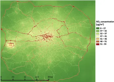
The baseline RapidAir kernel model (i.e. model not including urban morphology effects) highlighted expected contributions to NOx con-centrations from major roads in London, and Heathrow airport in the west of the study area (Fig. A10). The modelled concentrations at the monitoring sites were extracted and showed that the RapidAir model systematically underestimated observed NOxconcentrations (Table 1). Possible causes of this model underestimation are discussed further below.

Using a similar conceptual approach toGulliver and Briggs (2011), we corrected our modelled concentrations to account for potential systematic linear biases by linear regression between modelled and observed NOx. The receptor locations were randomly split intotraining (n= 57) and test (n= 29) data sets, with the latter used as an in-dependent verification data set. The linear regression using thetraining data (Fig. 1) was:

= ∗

Measured NOx 1.98 Kernel modelled NOx [4] WhereMeasured NOxandKernel modelled NOxare concentrations inμg/ m3_.

A map of the modelled NOxconcentrations in the study area after correction for the systematic biases discussed previously is provided in Fig. A10.

3.1.1. Discussion of causes of systematic bias in air pollution models Dispersion modelling involves multiple data inputs over several stages, any of which has potential to contribute to inaccuracies in pollution estimates. The under-prediction of NOxconcentrations in our analyses may be due to uncertainties in emissions and/or meteor-ological data, and/or uncertainties of representation of physical pro-cesses in AERMOD. The simplest errors to characterise are for road traffic emissions and meteorology data.

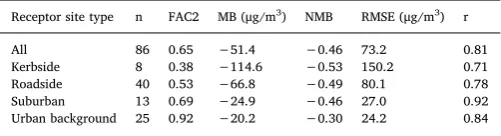
It is likely that road traffic NOxemissions data are underestimated in LAEI inventory we used. This inventory was prepared by a statutory body (Greater London Authority [GLA]) and remains the officially re-cognised emissions dataset for London. The European Environment Agency's COPERT road traffic emissions model, which was used by GLA to create the LAEI, has been observed to under-predict historical NOx emissions from diesel vehicles in the UKfleet (Carslaw et al., 2011). Consequently, it is likely that reported under-prediction of emissions in the dieselfleet biases the inventory towards under-prediction of at-mospheric concentrations. NOxemissions in the GLA inventory are re-ported to have been underestimated by approximately 31% in 2008 (Beevers et al., 2012b), consistent with predictions of a coupled re-gional CMAQ and road source dispersion model (CMAQ-urban) Table 1

Model evaluation statistics for measured NOxvs.unadjusted RapidAir modelled

NOx.

Receptor site type n FAC2 MB (μg/m3_{) NMB RMSE (μg/m}3_{) r}

All 86 0.65 −51.4 −0.46 73.2 0.81

Kerbside 8 0.38 −114.6 −0.53 150.2 0.71

Roadside 40 0.53 −66.8 −0.49 80.1 0.78

Suburban 13 0.69 −24.9 −0.46 27.0 0.92

Urban background 25 0.92 −20.2 −0.30 24.2 0.84

FAC2= fraction of modelled concentrations falling within a factor of 2 of the measured concentrations; MB= mean bias; NMB= normalised mean bias;

developed by other researchers for London [average NOx under-estimation by CMAQ-urban of 32% (Beevers et al., 2012a)]. A correc-tion for 31% underestimated emissions in our analyses would change the slope of modelled vs. observed concentrations (= 1/1.98) in the training dataset regression analyses above from 0.51 (49% under-estimation of observations) to 0.73 (27% underunder-estimation), which is of a consistent magnitude with the above underestimation of CMAQ-urban modelledvs.observed NOxconcentrations calculated byBeevers et al., (2012a). The effect of using the most recent release of COPERT road traffic emissions model on the emissions in London is discussed further in theAppendix(andTable A2).

Meteorological input data is a further potentially important source of systematic bias - concentrations are inversely proportional to wind speed in the Gaussian dispersion equation meaning uncertainties in wind speed estimates can lead to model bias. For example,Gulliver and Briggs (2011) noted that differences in windspeed measured at the

relatively open Heathrow airport meteorological station and wind-speeds measured during short duration periods at pollution monitoring sites in central London resulted in PM10 model predictions using windspeeds measured in central London being on average 67.5% lower than PM10 predicted using windspeeds measured at Heathrow. Simi-larly,Beevers et al. (2012a)noted that windspeeds measured at Hea-throw were systematically higher than windspeeds forecast using the Weather Research Forecast (WRF) model. Specifically, Beevers et al. illustrate how average midday windspeeds for 2006 measured at Hea-throw and modelled by WRF were∼5 m/s and∼3.5 m/s respectively (difference representing∼43% of WRF estimate approximated from Fig 7 inBeevers et al., 2012a). These differences suggest that use of mea-sured Heathrow windspeed data could result in an approximate 30% underestimation of pollution concentrations compared to equivalent concentrations estimated using WRF windspeed data. The impact of using wind speeds from modelvs.Heathrow for our study period and Fig. 1.Scatter plot of Measured vs. unadjusted RapidAir modelled NOxconcentrations for randomly selected training subset of receptors (n = 57).

the consequent impact on the kernels created is discussed further in the Appendix(andFigs A7 to A9, andTable A3).

The multiplicative combination of ∼31% underestimated NOx emissions from the LAEI and∼43% higher windspeeds from London Heathrow measurements (cf.WRF windspeed estimates used byBeevers et al., 2012a) suggests that the RapidAir pollution estimates in our analyses may have underestimated NOxconcentration observations in central London by approximately 48% (≡ 0.69/1.43) in context of above equivalent model-observation comparisons made for CMAQ-Urban (Beevers et al., 2012a). This difference is of similar magnitude to the underestimation of initial RapidAir model estimates compared to monitoring site observations (e.g. underestimation of 49% of observed concentrations represented inFig. 1).

3.2. RapidAir model evaluation–NO2

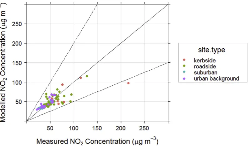
Concentrations of NO2 estimated from RapidAir (Fig. 2) were compared to NO2concentrations measured at the receptor locations in Table A1.

NO2concentrations predicted by RapidAir were similar to measured NO2concentrations at most monitoring stations; however the model underestimated concentrations at some very high concentration kerb-side measurement sites (Fig. 3,Table 2a). Underestimation by RapidAir model might be attributed to urban morphologies (including street canyon effects) or underestimation in the location-specific emissions rates used to predict the NOxconcentrations (Beevers et al., 2012b). The correlation between modelled and observed NO2concentrations (r= 0.77) was of similar magnitude to previous evaluations of disper-sion models (e.g.r= 0.74 reported byde Hoogh et al. (2014)during evaluation of a NOxdispersion model in the ESCAPE study).

DEFRA suggest that an air quality model is‘acceptable’for use if more than half of its observations fall within a factor of 2 of the ob-servations (Williams et al., 2011). The NO2RapidAir model meets the FAC2criterion for all site types, with the lowest FAC2 value calculated for kerbside sites (FAC2 = 0.88) (Table 2a). Kerbside concentrations represent the worst-case exposure scenarios that are not representative of population exposures over extended periods, and consequently an-nual limit values do not apply at these sites (DEFRA, 2016). Similar findings were reported in the DEFRA urban model evaluation exercise

for NO2which found thatFAC2values were lower for the kerbside sites than the three other site types tested, however all models met the above DEFRA criterion at the different site types (Carslaw, 2011). Another criterion suggested by DEFRA to indicate the acceptability of a model is that NMBvalues should lie between−0.2 and 0.2 (Williams et al., 2011).NMBvalues for RapidAir met this criterion when all sites were considered together; and for the individual site types, with the excep-tion of the kerbside sites (Table 2a). None of the models tested during the DEFRA model evaluation exercise met theNMB‘acceptance values’

proposed by DEFRA at the kerbside sites (Carslaw, 2011). The numbers of models meeting the criteria was progressively higher for kerbside, roadside and urban background site classifications–with all models meeting the NMBcriterion at urban background locations (Carslaw, 2011).

3.3. Accounting for street canyon effects in RapidAir

We investigated the inclusion of two techniques within the RapidAir model to describe the effects of street canyons on pollution con-centrations. Thefirst technique used geospatial surrogates to account for building morphologies within a study area, and the second applied industry-standard street canyon models to user-defined street canyon geometries. These techniques are discussed in the following sub-sec-tions.

3.3.1. GIS-surrogates for street canyons

We investigated if street canyon surrogates measured at each re-ceptor could be used to estimate, and subsequently correct for, the ef-fects of urban morphology on modelled NOxconcentrations, and NOx concentrations converted to NO2concentrations using the method de-scribed above.

The NOx receptors were split randomly into the same training (n= 57) andtest(n= 29) datasets used to derive the OLS correction for bias described at the start of Section3, with the former used to develop surrogate-correction equations and the latter used as an independent dataset to test the correction equations derived. A multiple-linear ca-libration equation was derived between Unadjusted modelled NOx, measured NOxandSurrogatefor each of the three surrogate values in-vestigated using thetrainingdataset (Table 3a).

Fig. 3.Scatter plot of NO2estimated by bias-corrected RapidAir kernel modelvs. observed concentrations at measurement stations (n = 86). Receptors are colour

The multiple linear calibrations developed were then applied to the testNOx.Table 3b shows theMeasuredvs.ModelledNOxafter applica-tion of the surrogate calibraapplica-tions for thetestdataset. The correlation between the concentrations and surrogates was unaffected by the sur-rogate used (r= 0.75).

3.3.2. Street canyon models

Of the 86 receptor locations we identified 19 sites that were located within urban street canyons through observations of the urban mor-phology using GIS and Google Maps Street View (Map data ©₂₀₁₇ Google) (Table A1).

A representative subset of the annual hourly meteorological data was used in the street canyon models to reduce model run times (dis-cussed inAppendix A). The effect of using a subset of meteorological data on computed annual average concentrations compared to the whole dataset was minimal for both canyon models. AEOLIUS was slightly more sensitive to the use of a sampled meteorological record (STREET model: slope = 1.00, intercept =−0.21,R2_{= 1.00; AEOLIUS} model: slope = 0.91, intercept = 0.71,R2= 0.99) (Fig. A11).

The windward and leeward concentrations predicted by each of the street canyon models were averaged on the assumption that over a year concentrations are well mixed within the street canyon. The con-centrations predicted within by the canyon model were then added to the baseline NOxconcentrations predicted by the RapidAir model (re-presenting the urban background in the area), and the models corrected Table 2

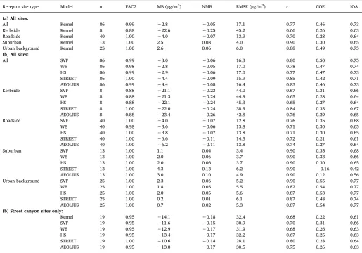
Summary model evaluation statistics for annual mean NO2at receptor locations (trainingandtestdata combined) split by site type: (a) kernel model only (all sites);

(b) kernel model with surrogate or street canyon correction (all sites); and (c) street canyon sites only. Statistics are given for the bias corrected Kernel only model, the kernel model after correction using the surrogates for street canyons and then bias corrected, and using the street canyon models with bias correction. SeeTable 1

caption for a description of the abbreviations used in the column headings.

Receptor site type Model n FAC2 MB (μg/m3_{) NMB RMSE (μg/m}3_{) r COE IOA}

(a) All sites:

All Kernel 86 0.99 −2.8 −0.05 17.1 0.77 0.46 0.73

Kerbside Kernel 8 0.88 −22.6 −0.25 45.2 0.66 0.26 0.63

Roadside Kernel 40 1.00 −4.0 −0.07 13.9 0.70 0.28 0.64

Suburban Kernel 13 1.00 2.5 0.08 4.0 0.90 0.30 0.65

Urban background Kernel 25 1.00 2.6 0.06 6.0 0.88 0.49 0.75

(b) All sites:

All SVF 86 0.99 −3.0 −0.06 16.3 0.80 0.50 0.75

WE 86 0.98 −2.8 −0.05 17.0 0.78 0.47 0.74

HS 86 0.99 −2.9 −0.06 17.0 0.77 0.47 0.73

STREET 86 1.00 −4.4 −0.09 15.9 0.85 0.42 0.71

AEOLIUS 86 0.99 −4.4 −0.08 16.4 0.83 0.46 0.73

Kerbside SVF 8 0.88 −21.1 −0.23 44.0 0.67 0.31 0.66

WE 8 0.88 −21.3 −0.24 44.9 0.65 0.28 0.64

HS 8 0.88 −22.1 −0.24 45.3 0.65 0.27 0.64

STREET 8 1.00 −22.0 −0.24 38.9 0.84 0.33 0.67

AEOLIUS 8 0.88 −23.4 −0.26 42.8 0.76 0.29 0.65

Roadside SVF 40 1.00 −4.0 −0.07 12.8 0.76 0.35 0.68

WE 40 0.98 −3.6 −0.06 13.8 0.71 0.30 0.65

HS 40 1.00 −3.8 −0.07 13.8 0.71 0.30 0.65

STREET 40 1.00 −6.6 −0.11 14.3 0.72 0.21 0.61

AEOLIUS 40 1.00 −6.2 −0.11 13.8 0.74 0.27 0.64

Suburban SVF 13 1.00 1.1 0.04 3.4 0.90 0.35 0.68

WE 13 1.00 2.0 0.06 3.7 0.90 0.33 0.66

HS 13 1.00 2.0 0.06 3.7 0.90 0.30 0.65

STREET 13 1.00 4.3 0.13 6.2 0.90 −0.16 0.42

AEOLIUS 13 1.00 3.0 0.10 4.9 0.90 0.12 0.56

Urban background SVF 25 1.00 2.3 0.06 5.2 0.90 0.55 0.77

WE 25 1.00 1.8 0.05 5.5 0.87 0.54 0.77

HS 25 1.00 2.0 0.05 5.6 0.87 0.53 0.77

STREET 25 1.00 0.2 0.01 6.1 0.87 0.48 0.74

AEOLIUS 25 1.00 0.7 0.02 5.3 0.87 0.54 0.77

(b) Street canyon sites only:

Kernel 19 0.95 −14.1 −0.18 32.4 0.68 0.22 0.61

SVF 19 0.95 −11.6 −0.15 30.9 0.70 0.31 0.66

WE 19 0.95 −12.9 −0.17 31.9 0.68 0.26 0.63

HS 19 0.95 −13.4 −0.17 32.2 0.67 0.25 0.63

STREET 19 1.00 −10.6 −0.14 28.1 0.80 0.28 0.64

AEOLIUS 19 0.95 −13.0 −0.17 30.5 0.75 0.26 0.63

Table 3

(a) Linear regression equations between measured NOx, kernel model NOx

(RapidAir_NOx) concentrations and the surrogate variables for thetrainingdata

set (n = 59), used to obtain a surrogate-adjusted RapidAir NOxconcentration

(‘Surrogate’_Adj_Mod_NOx); (b) Ordinary least squares regression equations

be-tween the measured (Measured_NOx) and surrogate-adjusted kernel model NOx

concentrations (baseline and after surrogate correction) for thetestdata set (the intercepts were insignificant therefore set to 0) (n = 29).

Surrogate (a)Training data:

Equations for surrogate-adjusted RapidAir NOx(μg/m3)

r

RapidAir RA_Adj_Mod_NOx= 1.98*RapidAir_NOx 0.93 SVF SVF_Adj_Mod_NOx= 1.87*RapidAir_NOx–

70.61*SVF + 55.90

0.84

WE WE_Adj_Mod_NOx= 2.00*RapidAir_NOx– 90.99*WE + 85.43

0.84

HS HS_Adj_Mod_NOx= 2.01*RapidAir_NOx– 54.04*HS + 49.57

0.83

Surrogate (b)Test data:

Measured vs Modelled NOx(μg/m3)

r

RapidAir Measured NOx= 0.79*RA_Adj_Mod_NOx 0.86 SVF Measured_NOx= 0.79*SVF_Adj_Mod_NOx 0.87

WE Measured_NOx= 0.78*WE_Adj_Mod_NOx 0.85

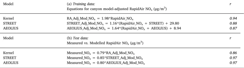
for systematic bias following the guidance in DEFRA Technical Guidance 2016 (DEFRA, 2016) (Table 4).

3.3.3. Evaluation of RapidAir NO2 estimates after accounting for street canyon effects

At the receptor locations in street canyons the underestimation of the receptor concentrations was lowest for the street canyon models, with the surrogates model and kernel models similarly under predicting the concentrations (NO2NMB =−0.18 for kernel, average NMB -0.16 for surrogates, −0.14 for STREET and −0.17 for AEOLIUS models (n = 19)) (Table 2b (NO2) andTable A4(NOx)). The STREET model predicted higher concentrations than the AEOLIUS model which re-sulted in the smaller NMB values (Fig. A12). The difference in modelled concentrations between the STREET and AEOLIUS models was very small which is similar to previously published findings (Ganguly and Broderick, 2011,2010;Gualtieri, 2010;Zhu et al., 2015).

When all types of receptor locations were considered, there was little difference between the pollution concentrations estimated at the receptor locations for the RapidAir model, surrogates and the street canyon models (Fig. A13). Consequently, there was limited difference in the model evaluation statistics when the surrogates and street canyon models were included (Table 2b (NO2) andTable A4(NOx)). Inclusion of the street canyon models reduced the NO2NMB values compared to the standard kernel model, however inclusion of the surrogates had little impact on NMB values at the kerbside sites (Kernel =−0.25, Surrogates =−0.24, STREET =−0.24 and AEOLIUS =−0.26) (Table 2b (NO2) and Table A4 (NOx)). LUR models for NO2 in-corporatingSVFstreet canyon surrogates also found little improvement in coefficient of determination values after surrogate inclusion (R2_{= 0.76vs.0.78) (Eeftens et al., 2013).}

Despite the negligible change in model evaluation statistics the combined kernel-canyon models required less adjustment for sys-tematic bias than the uncorrected kernel model (Table 4). Therefore, when a combined kernel-canyon model is applied to areas of the city which do not have any measurements the model may be subject to less over or under estimation than the kernel model which does not attempt to address urban morphology. For instance, the combined kernel-STREET model required adjustment using the linear regression equa-tionAdjusted NOX=1.04 * Modelled NOx+34.45.The slope here is significantly lower than the regression equation used to correct the kernel-only model (i.e. 1.04 vs.1.98). Predicted concentrations were similar for the combined kernel-STREET and combined kernel-AEOLIUS models. The inclusion of the street canyon models is therefore an im-portant step in accounting for urban morphology which can in practice be as influential to air pollution concentrations as spatial variations in emissions in an urban setting.

The use of surrogates to account for urban morphology effects,

including street canyons, has computational simplicity advantages over street canyon models. Surrogate values can be rapidly calculated in a GIS across a large study area. Canyon models require user selection of canyon locations, and require additional information about canyon widths, heights, and traffic information such as speed (and therefore cannot be easily computed for large areas).

Additionally, the transition from‘built up’to‘open’within the city (for example at boundaries between buildings and parkland) is treated in a gradual manner in surrogate models - unlike street canyon models which impose a hard boundary at the canyon edge which is‘smoothed’

artificially in a GIS with interpolation routines. Currently surrogates do not take wind speed into account which, for annual averages, we an-ticipate to have little influence on the model accuracy. However, if the surrogates were to be applied to a dispersion model with higher (e.g. hourly) temporal resolution then some modification of the surrogates to account for wind speed effects may be required in order to obtain si-milar modelled and measured pollution concentrations.

3.4. Advantages and limitations of RapidAir

The main aim of this work was to evaluate an air quality modelling platform designed for operational settings where time is often a priority and manpower/computational resources are limited. An example of an operational use of RapidAir is given inAppendix A. RapidAir succeeds as an operational air quality model in the context of very large urban areas and as a decision support tool but its efficiency comes with some drawbacks. Therefore, it is appropriate to outline the key benefits and limitations of the approach to enable practitioners to interpret this work in light of their current experiences in running city scale dispersion models.

Clearly a significant benefit with RapidAir is reduced computational burden. Run times of 10 min or less for a very large city with > 8 million inhabitants present a significant benefit for the operational modeller and decision makers who require fast but robust analyses. The RapidAir platform allows extremely efficient policy testing and other

“what if”model runs for new emission scenarios to be undertaken in a few minutes on a standard office computer which is to our knowledge not possible using existing platforms.

The model performance metrics for RapidAir inTable 2 are very similar to those computed for other dispersion modelling systems in the DEFRA inter comparison exercise. For example, the RapidAir outputs for kerbside locations in London have NO2 RMSE values of 38.91–45.26μg/m3 _{depending on the method taking street canyons} into consideration (r = 0.65–0.84, n = 8) where the models in the inter comparison have RMSE values ranging from 29.39 to 67.09μg/m3 (r = 0.15–0.93, n = 7). At roadside locations the RapidAir outputs have NO2RMSE values of 12.78–14.28μg/m3_{(r = 0.70–0.76, n = 40) where} Table 4

(a) Linear adjustment equations to account for systematic bias in kernel model performance. This data was derived from thetraining

dataset (n = 59). Equations are shown for the kernel model; and kernel model including street canyon model. The intercept was not significant for kernel and therefore the intercept was forced through the origin. (b) Ordinary least squares regression equations between the measured (Measured_NOx) and canyon-adjusted kernel model NOxconcentrations (baseline and after canyon correction)

for thetestdata set (the intercepts were insignificant therefore set to 0) (n = 29).

Model (a)Training data:

Equations for canyon model-adjusted RapidAir NOx(μg/m3)

r

Kernel RA_Adj_Mod_NOx= 1.98*RapidAir_NOx 0.94

STREET STREET_Adj_Mod_NOx= 1.16*(RapidAir_NOx+ STREET) + 29.80 0.88

AEOLIUS AEOLIUS_Adj_Mod_NOx= 1.64*(RapidAir_NOx+ AEOLIUS) + 8.94 0.87

Model (b)Test data:

Measured vs. Modelled RapidAir NOx(μg/m3)

r

Kernel Measured_NOx= 0.79*RA_Adj_Mod_NOx 0.86

STREET Measured_NOx= 0.85*STREET_Adj_Mod_NOx 0.97

the models in the inter comparison have RMSE values ranging from 9.94 to 19.69μg/m3 (r = 0.38–0.89, n = 30). Some of the variation between RapidAir and the other models will be due to the different number of receptors in each category (which in reality may help or hinder our model performance) but it is impossible for us to match the locations exactly for the reasons explained earlier. The model results also yielded good results for the COE and IOA when compared with the definitions for these metrics provided byCarslaw and Ropkins (2012). The key model metrics for the 2008 model run in London are very si-milar to standard modelling suites used in the UK and which are used and accepted by DEFRA for use in compliance assessments at the highest level of statutory European air quality reporting. The high spatial resolution possible with the RapidAir model makes it a suitable candidate for use as an exposure metric for epidemiology studies for example.

In our view the potential drawbacks of the model must be balanced against the benefits described above. There may be the suggestion that the kernel based model represents a significantly simplified treatment of urban dispersion compared with models currently in use in the UK which iterate over thousands of receptors and calculate contributions at those receptors as a function of those sources (with very significant run times). In fact, all Gaussian and empirical models are already a greatly simplified picture of reality in urban settings and the methodology in RapidAir does not significantly alter the overall level of simplification compared with the real situation. In any case the model results are compared against pollution measurements as with all other models using the same metrics and the results of that performance assessment are comparable with other platforms.

The performance statistics for the surrogates for urban morphology are reasonably close to those from the models which treat canyons discretely. Again our focus is on operational modelling where re-producible and efficient workflows are as important as the tools se-lected for use. Based on this work we would suggest that for compliance assessment RapidAir is used with either the STREET or AEOLIUS model options included as the run times are not significantly impacted by including these models. The model results should be compared with measured concentrations and the modeller may choose the best per-forming street canyon model for their case. The surrogate models should be used as screening tools and perhaps to spatially delineate locations where the street canyon models should be invoked, which is often difficult for a large and complex urban environment where re-sources do not permit thorough investigation and spatial treatment of the morphological conditions.

4. Conclusions

We developed a kernel-based dispersion model (RapidAir) com-bining AERMOD and open-source scientific computing methods to es-timate pollution concentrations atfine spatial resolution. Model input data was obtained from public sources to allow comparison with pol-lution models for the same location with the same input data. The RapidAir dispersion model took approximately 7 min to model the Greater London conurbation (∼3500 km2

) at 5 × 5 m resolution using an Intel i5 64-bit laptop with 8 Gb RAM.

We evaluated NOxand NO2 model predictions at 86 sites across London. After correction for systematic under estimation bias in the initial RapidAir model, FAC2 values for modelled concentrations were > 0.85 at the 86 evaluation sites. RMSE values decreased through the site categories: Kerbside, Roadside, Urban Background and Suburban (RMSE = 45, 14, 6 and 4μg/m3respectively). Thisfinding is consistent with results from other modelling groups participating in the DEFRA inter comparison, whose RMSE values ranged from 3 to 70μg/ m3respectively.

The larger RMSE values at the sites in proximity to traffic sources may have resulted from the presence of street canyons that trap pol-lutants leading to elevated concentrations –an effect that cannot be

described in dispersion models unless urban morphologies are taken into consideration. Correspondingly, we used geospatial surrogates (sky-view factor, hill shading and wind effect) and separate street canyon models (STREET and AEOLIUS) to improve modelled con-centrations at roadside sites. The STREET canyon model and street canyon surrogates improved the model RMSE at kerbside sites: RapidAir base-kernel = 45.2, sky-view factor surrogate = 44.0, STREET model = 38.9 and AEOLIUS = 42.8μg/m3. When all sites were considered the lowest RMSE values were observed for the kernel model combined with the STREET canyon model (RMSE RapidAir base-kernel = 17.1 vs. STREET model = 15.9μg/m3). Consequently, the combined models may be anticipated to provide more accurate esti-mates when extrapolated to locations without monitoring. The geos-patial surrogates have potential as simple means of incorporating canyon effects into a large city scale dispersion model. The advantage of using simple geospatial surrogates for street canyons instead of mod-elling canyons discretely include: reduced run times, smaller user input required and the transition from‘built up’to‘open’environments is treated gradually.

Acknowledgements

We gratefully acknowledge the work of Professor Bryan Harris at the University of Bath, who previously developed a Mathcad version of the AEOLIUS model and who diligently described the model formula-tions he obtained from the Met Office's original author Dr D. R. Middleton; and much of our implementation of the AEOLIUS model is based on Professor Harris' description of the system of equations which make up AEOLIUS (Harris, 2004) (seeAppendix A).

Nicola Masey is funded through a UK Natural Environment Research Council CASE PhD studentship (NE/K007319/1), with support from Ricardo Energy and Environment. We acknowledge access to the LAQN measurement data, and the PCM model data, which were obtained from uk-air.defra.gov.uk and are subject to Crown 2014 copyright, Defra, licensed under the Open Government Licence (OGL). RapidAir®is a registered trade mark of Ricardo-AEA Limited, used under permission of Ricardo-AEA Limited.

Appendix A. Supplementary data

Supplementary data related to this article can be found athttp://dx. doi.org/10.1016/j.envsoft.2018.05.014.

References

Beevers, S.D., Kitwiroon, N., Williams, M.L., Carslaw, D.C., 2012a. One way coupling of CMAQ and a road source dispersion model forfine scale air pollution predictions. Atmos. Environ. 59, 47–58.http://dx.doi.org/10.1016/j.atmosenv.2012.05.034. Beevers, S.D., Westmoreland, E., de Jong, M.C., Williams, M.L., Carslaw, D.C., 2012b.

Trends in NOx and NO2 emissions from road traffic in Great Britain. Atmos. Environ. 54, 107–116.http://dx.doi.org/10.1016/j.atmosenv.2012.02.028.

Bellander, T., Berglind, N., Gustavsson, P., Jonson, T., Nyberg, F., Pershagen, G., Järup, L., 2001. Using geographic information systems to assess individual historical ex-posure to air pollution from traffic and house heating in Stockholm. Environ. Health Perspect. 109, 633–639.

Berkowicz, R., 2000. OSPM - a parameterised street pollution model. Environ. Monit. Assess. 65, 323–331.http://dx.doi.org/10.1023/A:1006448321977.

Böhner, J., Antonić, O., 2009. Chapter 8 land-surface parameters specific to topo-clima-tology. In: Reuter, T.H., H.I. (Eds.), Developments in Soil Science,

GeomorphometryConcepts, Software, Applications. Elsevier, pp. 195–226.http://dx. doi.org/10.1016/S0166-2481(08)00008-1.

Briggs, D., Collins, S., Elliott, P., Fischer, P., Kingham, S., Lebret, E., Pryl, K., Van Reeuwijk, H., Smallbone, K., Van Der Veen, A., 1997. Mapping urban air pollution using GIS: a regression-based approach. Int. J. Geogr. Inf. Sci. 11, 699–718. Buckland, A.T., 1998. Validation of a street canyon model in two cities. Environ. Monit.

Assess. 52, 255–267.http://dx.doi.org/10.1023/A:1005828128097.

Buckland, A.T., Middleton, D.R., 1999. Nomograms for calculating pollution within street canyons. Atmos. Environ. 33, 1017–1036. http://dx.doi.org/10.1016/S1352-2310(98)00354-9.

340–348.http://dx.doi.org/10.1016/j.enbuild.2014.10.001.

Carslaw, D., 2011. Defra Urban Model Evaluation Analysis - Phase 1. King’s College London. https://uk-air.defra.gov.uk/library/reports?report_id=654. Carslaw, D., Beevers, S.D., Westmoreland, E., Williams, M., Tate, J., Murrells, T.,

Stedman, J., Li, Y., Grice, S., Kent, A., Tsagatakis, I., 2011. Trends in NOx and NO2 emissions and ambient measurements in the UK.https://uk-air.defra.gov.uk/library/ reports?report_id=645.

Carslaw, D.C., Ropkins, K., 2012. Openair—an R package for air quality data analysis. Environ. Model. Software 27–28, 52–61.http://dx.doi.org/10.1016/j.envsoft.2011. 09.008.

Chang, J.C., Hanna, S.R., 2004. Air quality model performance evaluation. Meteorol. Atmos. Phys. 87, 167–196.http://dx.doi.org/10.1007/s00703-003-0070-7. Conrad, O., Bechtel, B., Bock, M., Dietrich, H., Fischer, E., Gerlitz, L., Wehberg, J.,

Wichmann, V., Boehner, J., 2015. System for automated geoscientific analyses (SAGA) v. 2.1.4. Geosci. Model Dev. 8, 1991–2007. http://dx.doi.org/10.5194/gmd-8-1991-2015.

Dabberdt, W.F., Ludwig, F.L., Johnson, W.B., 1973. Validation and applications of an urban diffusion model for vehicular pollutants. Atmos. Environ. 1967 (7), 603–618. http://dx.doi.org/10.1016/0004-6981(73)90019-X.

de Hoogh, K., Korek, M., Vienneau, D., Keuken, M., Kukkonen, J., Nieuwenhuijsen, M.J., Badaloni, C., Beelen, R., Bolignano, A., Cesaroni, G., Pradas, M.C., Cyrys, J., Douros, J., Eeftens, M., Forastiere, F., Forsberg, B., Fuks, K., Gehring, U., Gryparis, A., Gulliver, J., Hansell, A.L., Hoffmann, B., Johansson, C., Jonkers, S., Kangas, L., Katsouyanni, K., Künzli, N., Lanki, T., Memmesheimer, M., Moussiopoulos, N., Modig, L., Pershagen, G., Probst-Hensch, N., Schindler, C., Schikowski, T., Sugiri, D., Teixidó, O., Tsai, M.-Y., Yli-Tuomi, T., Brunekreef, B., Hoek, G., Bellander, T., 2014. Comparing land use regression and dispersion modelling to assess residential ex-posure to ambient air pollution for epidemiological studies. Environ. Int. 73, 382–392.http://dx.doi.org/10.1016/j.envint.2014.08.011.

DEFRA, 2017a. The data verification and ratification process [www Document].https:// uk-air.defra.gov.uk/assets/documents/The_Data_Verification_and_Ratification_ Process.pdf, Accessed date: 4 January 2017.

DEFRA, 2016. Local Air Quality Management Technical Guidance (TG16) (No. TG16). Defra. https://laqm.defra.gov.uk/technical-guidance/.

DEFRA, 2017b. NOx to NO2 tool version 3.2. https://laqm.defra.gov.uk/review-and-assessment/tools/background-maps.html, Accessed date: 20 March 2017. DEFRA, 2018. URLhttps://uk-air.defra.gov.uk/data/modelling-data(accessed 27.03.

2018).

Derwent, D., Fraser, A., Abbott, J., Jenkin, M., Willis, P., Murrells, T., 2010. Evaluating the Performance of Air Quality Models. Defra (No. Issue 3).

Dons, E., Int Panis, L., Van Poppel, M., Theunis, J., Wets, G., 2012. Personal exposure to Black Carbon in transport microenvironments. Atmos. Environ. 55, 392–398.http:// dx.doi.org/10.1016/j.atmosenv.2012.03.020.

Dons, E., Van Poppel, M., Int Panis, L., De Prins, S., Berghmans, P., Koppen, G., Matheeussen, C., 2014a. Land use regression models as a tool for short, medium and long term exposure to traffic related air pollution. Sci. Total Environ. 476–477, 378–386.http://dx.doi.org/10.1016/j.scitotenv.2014.01.025.

Dons, E., Van Poppel, M., Kochan, B., Wets, G., Int Panis, L., 2014b. Implementation and validation of a modeling framework to assess personal exposure to black carbon. Environ. Int. 62, 64–71.

Earth Systems Research Laboratory NOAA, 2018. URLhttp://www.esrl.noaa.gov/raobs/ (accessed 27.03.2018).

Eeftens, M., Beekhuizen, J., Beelen, R., Wang, M., Vermeulen, R., Brunekreef, B., Huss, A., Hoek, G., 2013. Quantifying urban street configuration for improvements in air pollution models. Atmos. Environ. 72, 1–9.http://dx.doi.org/10.1016/j.atmosenv. 2013.02.007.

Emu Analytics, 2018. URLhttp://buildingheights.emu-analytics.net/(accessed 27.03. 2018).

ESRI, 2014. ArcGIS Desktop Version 10.2.2. Environmental Systems Research Institute, CA, USA.

Fallah-Shorshani, M., Shekarrizfard, M., Hatzopoulou, M., 2017. Integrating a street-canyon model with a regional Gaussian dispersion model for improved character-isation of near-road air pollution. Atmos. Environ. 153, 21–31.http://dx.doi.org/10. 1016/j.atmosenv.2017.01.006.

Ganguly, R., Broderick, B.M., 2011. Application of urban street canyon models for pre-dicting vehicular pollution in an urban area in Dublin. Ireland. Int. J. Environ. Pollut 44, 71–77.http://dx.doi.org/10.1504/IJEP.2011.038404.

Ganguly, R., Broderick, B.M., 2010. Estimation of CO concentrations for an urban street canyon in Ireland. Air Qual. Atmosphere Health Dordr 3, 195–202.https://doi.org/ 10.1007/s11869-010-0068-5.

Gibson, M.D., Kundu, S., Satish, M., 2013. Dispersion model evaluation of PM2.5, NOx and SO2 from point and major line sources in Nova Scotia, Canada using AERMOD Gaussian plume air dispersion model. Atmospheric Pollut. Res. 4, 157–167.http:// dx.doi.org/10.5094/APR.2013.016.

Gillespie, J., Beverland, I.J., Hamilton, S., Padmanabhan, S., 2016. Development, eva-luation, and comparison of land use regression modeling methods to estimate re-sidential exposure to nitrogen dioxide in a cohort study. Environ. Sci. Technol. 50, 11085–11093.http://dx.doi.org/10.1021/acs.est.6b02089.

Gillespie, J., Masey, N., Heal, M.R., Hamilton, S., Beverland, I.J., 2017. Estimation of spatial patterns of urban air pollution over a 4-week period from repeated 5-min measurements. Atmos. Environ. 150, 295–302.http://dx.doi.org/10.1016/j. atmosenv.2016.11.035.

Gualtieri, G., 2010. A street canyon model intercomparison inflorence, Italy. Water Air Soil Pollut. Dordr 212, 461–482.https://doi.org/10.1007/s11270-010-0360-x. Gulliver, J., Briggs, D., 2011. STEMS-Air: a simple GIS-based air pollution dispersion

model for city-wide exposure assessment. Sci. Total Environ. 409, 2419–2429.

Harris, B., 2004. An Implementation of the OSPM/AEOLIUS air pollution model in MATHCAD and its application for a small Wiltshire town [WWW Document].web. onetel.com/∼bandmaharris/AeoliusInMathcad1.pdf, Accessed date: 20 March 2017. Hertel, O., Berkowicz, R., 1989. Modelling Pollution from Traffic in a Street Canyon:

Evaluation of Data and Model Development.http://dx.doi.org/10.13140/RG.2.1. 2251.6326.Rep. DMU LUFT A129.

Jackson, M., Hood, C., Johnson, C., Johnson, K., 2016. Calculation of urban morphology parameterisations for London for use with the ADMS-urban dispersion model. Int. J. Adv. Remote Sens. GIS 0, 1678–1687.

Johnson, M., MacNeill, M., Grgicak-Mannion, A., Nethery, E., Xu, X., Dales, R., Rasmussen, P., Wheeler, A., 2013. Development of temporally refined land-use re-gression models predicting daily household-level air pollution in a panel study of lung function among asthmatic children. J. Expo. Sci. Environ. Epidemiol. 23, 259–267. http://dx.doi.org/10.1038/jes.2013.1.

Johnson, W.B., Ludwig, F.L., Dabberdt, W.F., Allen, R.J., 1973. An urban diffusion si-mulation model for carbon monoxide. J. Air pollut. Control Assoc. 23, 490–498. http://dx.doi.org/10.1080/00022470.1973.10469794.

Kokalj, Z., Zaksek, K., Ostir, K., 2011. Application of sky-view factor for the visualisation of historic landscape features in lidar-derived relief models. Antiquity 85, 263–273. Kokalj, Z., Zaksek, K., Ostir, K., Pehani, P., Cotar, K., 2013. Relief Visualization Toolbox

Version 1.3 - Manual.

Korek, M., Johansson, C., Svensson, N., Lind, T., Beelen, R., Hoek, G., Pershagen, G., Bellander, T., 2016. Can dispersion modeling of air pollution be improved by land-use regression? An example from Stockholm, Sweden. J. Expo. Sci. Environ. Epidemiol.http://dx.doi.org/10.1038/jes.2016.40.

Lin, C., Feng, X., Heal, M.R., 2016. Temporal persistence of intra-urban spatial contrasts in ambient NO2, O3 and Ox in Edinburgh, UK. Atmospheric Pollut. Res. 7, 734–741. http://dx.doi.org/10.1016/j.apr.2016.03.008.

London Atmospheric Emissions Inventory, 2008. URLhttps://data.london.gov.uk/ dataset/laei-2008(accessed 27.03.2018).

London Datastore, 2016. Air quality summary statistics [www Document].https://data. london.gov.uk/dataset/air-quality-summary-statistics, Accessed date: 27 March 2018.

Manning, A.J., Nicholson, K.J., Middleton, D.R., Rafferty, S.C., 2000. Field study of wind and traffic to test a street canyon pollution model. Environ. Monit. Assess. 60, 283–313.http://dx.doi.org/10.1023/A:1006187301966.

Michanowicz, D.R., Shmool, J.L.C., Cambal, L., Tunno, B.J., Gillooly, S., Olson Hunt, M.J., Tripathy, S., NaumoffShields, K., Clougherty, J.E., 2016. A hybrid land use regres-sion/line-source dispersion model for predicting intra-urban NO2. Transport. Res. Part Transp. Environ 43, 181–191.http://dx.doi.org/10.1016/j.trd.2015.12.007. Middleton, D.R., 1999. Development of AEOLIUS for street canyon screening. Clean. Air

29, 155–161.

Middleton, D.R., 1998a. Dispersion Modelling: a Guide for Local Authorities, Met Office Turbulence and Diffusion Note Number 241. The Meteorological Office, Bracknell, Bercks.

Middleton, D.R., 1998b. A new box model to forecast urban air quality: boxurb. Environ. Monit. Assess. 52, 315–335.http://dx.doi.org/10.1023/A:1005817202196. Mukerjee, S., Smith, L., Neas, L., Norris, G., 2012. Evaluation of land use regression

models for nitrogen dioxide and benzene in four us cities. Sci. World J. 2012, e865150.http://dx.doi.org/10.1100/2012/865150.

National Climatic Data Centre NOAA, 2018.ftp://ftp.ncdc.noaa.gov/pub/data/noaa/, Accessed date: 27 March 2018.

Nyberg, F., Gustavsson, P., Järup, L., Bellander, T., Berglind, N., Jakobsson, R., Pershagen, G., 2000. Urban air pollution and lung cancer in Stockholm. Epidemiol. Camb. Mass 11, 487–495.

Patton, A.P., Zamore, W., Naumova, E.N., Levy, J.I., Brugge, D., Durant, J.L., 2015. Transferability and generalizability of regression models of ultrafine particles in urban neighbourhoods in the boston area. Environ. Sci. Technol. 49, 6051–6060. http://dx.doi.org/10.1021/es5061676.

Spinelle, L., Gerboles, M., Villani, M.G., Aleixandre, M., Bonavitacola, F., 2017. Field calibration of a cluster of low-cost commercially available sensors for air quality monitoring. Part B: NO, CO and CO2. Sensor. Actuator. B Chem. 238, 706–715. http://dx.doi.org/10.1016/j.snb.2016.07.036.

Spinelle, L., Gerboles, M., Villani, M.G., Aleixandre, M., Bonavitacola, F., 2015. Field calibration of a cluster of low-cost available sensors for air quality monitoring. Part A: ozone and nitrogen dioxide. Sensor. Actuator. B Chem. 215, 249–257.http://dx.doi. org/10.1016/j.snb.2015.03.031.

Su, J.G., Brauer, M., Ainslie, B., Steyn, D., Larson, T., Buzzelli, M., 2008a. An innovative land use regression model incorporating meteorology for exposure analysis. Sci. Total Environ. 390, 520–529.http://dx.doi.org/10.1016/j.scitotenv.2007.10.032. Su, J.G., Brauer, M., Buzzelli, M., 2008b. Estimating urban morphometry at the

neigh-bourhood scale for improvement in modeling long-term average air pollution con-centrations. Atmos. Environ. 42, 7884–7893.http://dx.doi.org/10.1016/j.atmosenv. 2008.07.023.

Survey Open Data, 2018. URLhttp://environment.data.gov.uk/ds/survey/index.jsp#/ survey(accessed 27.03.2018).

Tan, Y., Dallmann, T.R., Robinson, A.L., Presto, A.A., 2016. Application of plume analysis to build land use regression models from mobile sampling to improve model trans-ferability. Atmos. Environ. 134, 51–60.http://dx.doi.org/10.1016/j.atmosenv.2016. 03.032.

Tang, R., Blangiardo, M., Gulliver, J., 2013. Using building heights and street confi g-uration to enhance intraurban PM10, NOX, and NO2 land use regression models. Environ. Sci. Technol. 47, 11643–11650.http://dx.doi.org/10.1021/es402156g. Targa, J., Loader, A., 2008. Diffusion Tubes for Ambient NO2 Monitoring: a Practical

quality in street canyons: a review. Atmos. Environ. 37, 155–182.http://dx.doi.org/ 10.1016/S1352-2310(02)00857-9.

Wang, M., Beelen, R., Basagaña, X., Becker, T., Cesaroni, G., de Hoogh, K., Dėdelė, A., Declercq, C., Dimakopoulou, K., Eeftens, M., Forastiere, F., Galassi, C.,

Gražulevičienė, R., Hoffmann, B., Heinrich, J., Iakovides, M., Künzli, N., Korek, M., Lindley, S., Mölter, A., Mosler, G., Madsen, C., Nieuwenhuijsen, M., Phuleria, H., Pedeli, X., Raaschou-Nielsen, O., Ranzi, A., Stephanou, E., Sugiri, D., Stempfelet, M., Tsai, M.-Y., Lanki, T., Udvardy, O., Varró, M.J., Wolf, K., Weinmayr, G., Yli-Tuomi, T., Hoek, G., Brunekreef, B., 2013. Evaluation of land use regression models for NO2 and particulate matter in 20 european study areas: the ESCAPE project. Environ. Sci. Technol. 47, 4357–4364.http://dx.doi.org/10.1021/es305129t.

Williams, M., Barrowcliffe, R., Laxen, D., Monks, P., 2011. Review of Air Quality Modelling in Defra. Defra.

Wilton, D., Szpiro, A., Gould, T., Larson, T., 2010. Improving spatial concentration esti-mates for nitrogen oxides using a hybrid meteorological dispersion/land use

regression model in Los Angeles, CA and Seattle, WA. Sci. Total Environ. 408, 1120–1130.http://dx.doi.org/10.1016/j.scitotenv.2009.11.033.

Wong, D.W., Yuan, L., Perlin, S.A., 2004. Comparison of spatial interpolation methods for the estimation of air quality data. J. Expo. Sci. Environ. Epidemiol. 14, 404–415. http://dx.doi.org/10.1038/sj.jea.7500338.

World Health Organization, 2016. Ambient Air Pollution: a Global Assessment of Exposure and Burden of Disease. Geneva, Switzerland.

World Health Organization, 2013. Review of Evidence on Health Aspects of Air Pollution –REVIHAAP Project: Technical Report. Copenhagen, Denmark.

Zaksek, K., Ostir, K., Kokalj, Z., 2011. Sky-view factor as a relief visualization technique. Rem. Sens. 3, 398–415.http://dx.doi.org/10.3390/rs3020398.