The effect of extreme trim operation on propeller cavitation in self-propulsion conditions

A. Yücel Odabaşı Colloquium Series 3rd _{International Meeting - Progress in Propeller Cavitation and its Consequences:} Experimental and Computational Methods for Predictions 15th _{– 16}th _{November 2018, Istanbul, Turkey}

The Effect of Extreme Trim Operation on Propeller Cavitation in

Self-Propulsion Conditions

Matthias Maasch, Osman Turan and Sandy H. Day

Department of Naval Architecture and Marine Engineering, University of Strathclyde, 100 Montrose Street, Glasgow G4 0LZ, UK

Abstract: Experimental and numerical studies have shown that operating an LNG Carrier in extreme bow-up trim conditions can lead to substantial savings of over 25% in nominal ship resistance. The present study applies the Extreme Trim Concept to RANSE self-propulsion simulations including the prediction of propeller cavitation. It was investigated how the transient cavitation location and volume changed with varying ship displacements and trim angles over a range of ship speeds. Further, the effect of extreme trim and cavitation development on the ship delivered power was analyzed. Results have shown that by operating an LNG Carrier in extreme trim, power consumption and the extent of cavitation were reduced considerably. This study proved that the Extreme Trim Concept can be a valuable operating approach for reducing the environmental impact of LNG Carriers.

Keywords: Extreme Trim Concept, LNG Carrier, Self-propulsion simulation, Cavitation prediction.

1 INTRODUCTION

LNG Carriers operate a well-defined trading pattern in which a significant period of time is spent in unladen ballast conditions. During ballast voyage, in order to reach an operable ship draft, large amounts of ballast water are carried. Given that ballast water is unpaid load it is desirable to reduce the ballast loading while at the same time being operable on an efficient level. Therefore, the Extreme Trim Concept proposes to operate an LNG Carrier at extreme bow-up trim, thus realizing an operable draft at the aft, i.e. the propulsor is well submerged, with a minimum amount of ballast water carried. Previous experimental and numerical studies have shown that by applying extreme bow-up trim, over 25% reduction in nominal resistance compared to level trim operation is possible (Maasch et al., 2017).

Operating at an optimal trim at a constant displacement is thought to improve the flow field around the ship and hence decrease the wave making resistance. The impact on the frictional resistance component is marginal since, at a constant displacement, the hull wetted surface area does not change significantly. Another aspect of trim optimization is the influence on the propulsive performance, i.e. the inflow to the propeller and the propeller submergence. The latter often limits the range of bow-down trim angles to be tested since the propeller comes closer to the water surface with larger trim angles. (Reichel et al., 2014)

Experimental towing tank trim tests on the chosen LNG Carrier test case have shown that operating this ship at moderate trim angles either to stern or bow does not improve the ship’s performance significantly (Day et al., 2010). The same trend was validated by numerical

simulations. Hence, former results show that small changes to the ships trim do not have a positive effect on the wave making component of the total resistance or the propulsive performance, indicating that the hull is well designed for level trim operation at the tested loading condition. Mewis and Hollenbach outline that for each loading condition an ideal trim angle (including level trim) reduces the power consumption of a ship. In particular, modern cargo ships that feature a wide flat (submerged) transom and a pronounced bulbous bow do benefit from an optimized trim in off-loading conditions. (Mewis and Hollenbach, 2007)

Due to a small rotation of the hull (hydrostatic trim), a wet transom could emerge out of the water surface quite significantly, thus improving the wave making resistance. Also, a wide bulbous bow could be rotated to a more suitable water depth where its intended purpose of improving the bow free surface flow would be re-established. The LNG Carrier test case, however, operated in ballast loading conditions, features a dry and narrow flat transom and a relatively slender bulbous bow which could explain the hulls insensitivity to a standard trim optimization.

carrying large amounts of ballast water to operate at level trim conditions, the ballast water volume was reduced to a minimum in order to reach an extreme bow-up trim.

The present study extends the work published in (Maasch et al., 2017) by simulating the model scale LNG Carrier in four loading conditions over a speed range of 14-20 knots (full-scale) in self-propulsion conditions including propeller cavitation prediction.

2 NUMERICAL BACKGROUND

In order to investigate the effects of the Extreme Trim Concept on the propulsive performance of the LNG Carrier, numerical self-propulsion simulation at model scale were performed within this study.

This type of simulation, similar to self-propulsion towing tank experiments, is able to predict the performance of a vessel by simulating the hydrodynamic interaction of the hull, its propulsion system (in this CFD study the only relevant propulsion-system component was the propeller) and its rudder with each other and as a multi-component system with the environment, i.e. a domain of water and air. To solve the underlying flow physics, a state of the art commercial flow solver was used. In particular, the flow in the 3D dimensional numerical mesh was solved in time by an implicit unsteady flow scheme for the Reynolds-Averaged Navier-Stokes Equations (RANSE). In order to obtain a numerical solution for the flow field around a ship hull, the RANSE (see Eq. 1) solver allowed to divide the flow velocities and pressures into a time-averaged part (𝑢, 𝑣, 𝑤, 𝑝) and a fluctuating part (𝑢′_{, 𝑣}′_{, 𝑤}′_).

(1)

Here, the Reynolds stresses contain the turbulent fluctuations (see Eq. 2) that required a turbulence model in order to find a numerical solution. (Bertram, 2000a)

(2)

The turbulent flow was computed by the k-Omega SST model which blends the k-Epsilon model with the k-Omega model depending on the distance to the wall (i.e. ship hull). (SIEMENS, 2017a)

The free surface was solved using a Volume of Fluid (VOF) model under the assumption that both phases, water and air, share velocity and pressure (SIEMENS, 2017b). To be able to predict the generation of cavitation for different simulated loading conditions at various ship speeds, the transient growth and collapse of vapor volume in the computational domain needed to be accounted for in the Volume of Fluid model by an additional source term.

Since the standard formulation of the VOF method does not compute phase-transition, i.e. for a two-phase fluid including transition due to cavitation, a suitable cavitation model was added to the simulation setup (Schnerr and Sauer, 2001). The growth and collapse of vapor over time can be expressed by Eq. 3. For cavitation to occur, the vapor bubbles needed a surface on which to nucleate. Hence, a number (𝑁) of uniformly distributed seeds which provide that surface were required to be present in the computational domain.

𝑄𝑉= 𝑁 ∙ 4 ∙ 𝜋 ∙ 𝑅2∙ 𝑣𝑟 (3)

Assuming a spherical vapor bubble with the radius 𝑅, the bubble growth velocity 𝑣𝑟 remained as an unknown quantity in the physical setup. Further neglecting bubble-bubble interaction and bubble-bubble coalescence, the bubble-bubble growth velocity can be generally modelled by the Rayleigh-Plesset Cavitation Model (see Eq. 4).

𝑅𝑑𝑣𝑟 𝑑𝑡 +

3 2𝑣𝑟

2 ₌𝑝𝑆𝑎𝑡− 𝑝 𝜌𝑙

− 2 ∙ 𝜎 𝜌𝑙∙ 𝑅

− 4 𝜇𝑙 𝜑𝑙∙ 𝑅

𝑣𝑟 (4)

However, for a simulation case where the local pressure, e.g. at propeller blade depth, is sufficiently low and the pressure difference of local pressure and ambient pressure, e.g. at a larger distance to the propeller blade, is large, the reduced formulation of the Rayleigh-Plesset Cavitation Model, also called Schnerr-Sauer Cavitation Model can be applied to compute the bubble growth velocity. This simplified approach neglects the influence of bubble growth acceleration (𝑅 ∙ 𝑑𝑣𝑟/𝑑𝑡), viscous effects (4 ∙ 𝜇𝑙∙ 𝑣𝑟/(𝜑𝑙∙ 𝑅)) and the surface tension effects (2 ∙ 𝜎/(𝜌𝑙∙ 𝑅)), yielding Eq. 5. (SIEMENS, 2017c)

𝑣𝑟2= 2 3(

𝑝𝑆𝑎𝑡− 𝑝 𝜌𝑙

) (5)

The local pressure at the bubble boundary was represented by the saturation pressure 𝑝𝑆𝑎𝑡. With the above described setup, a number of self-propulsion simulation were performed to compute the required power delivered to the propeller and propeller cavitation.

3 SIMULATION SETUP

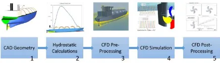
For setting up the self-propulsion simulations efficiently, repeatable steps in the pre-processing, the simulation run and the post-processing were automated. Therefore, a software chain was established as shown in Figure 11.

Figure 1 Automated Simulation Setup

of the LNG Carrier CAD model were calculated according to the draft at the aft perpendicular and the fore perpendicular where four sets of trim positions were considered as shown in Table 11.

Table 1 Loading Conditions, TL: Draft at fully laden conditions, TB: Draft at heavy ballast loading conditions

# ID Draft

Aft Fore

1 Fully Laden – Level Trim TL TL

2 Heavy Ballast – Level Trim TB TB

3 Min. Ballast – Extreme Trim TB 0

4 Heavy Ballast – Extreme Trim TL 0

Along with setting the hydrostatic floating position of the LNG Carrier, the CAD model was automatically divided in geometric parts so that custom meshing settings could be applied while generating the numerical mesh. Further, mesh refinement volumes were generated that adapted its shape to the ship hull for each loading condition automatically. Thus, the total number of cells in the numerical mesh was kept small. Figure 2 illustrates the refinement volume generation for two different loading conditions for the bow and the stern region.

Figure 2 Numerical Mesh Pre-processing

In particular, the figure shows how the refinement volume around the bow (green transparent shape) of the LNG Carrier adapts its shape to cover the region near the hull surface only.

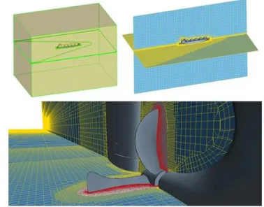
Figure 3 Global Numerical Mesh and Mesh Detail

In addition, global volumes for the numerical mesh control were prepared in the same manner. Refinement regions for the hull, the free surface, the rotating domain of the propeller and the ship wake were created automatically. Figure 3 shows the domain pre-processing in the top-left corner and the resulting numerical mesh from a global perspective in the top-right corner. A detailed view of the stern mesh and the rotating domain mesh is given as well. This approach allowed to produce a suitable numerical mesh of around 7 million cells, with approximately 4.3 million cells in the rotating domain, for each loading condition automatically.

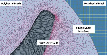
For the domain setup to be suitable to work as a numerical towing tank, the box shaped tank volume was set up consisting of velocity inlets at the front (upstream), the bottom and the top, a pressure outlet at the back (downstream) and symmetry planes at the sides (port and starboard). Using a velocity inlet condition allowed to avoid a velocity gradient between the fluid (either water or air) and the domain boundaries. The ship hull and its appendages, to allow interaction of the structure and the fluid, were of type no-slip wall. In order to simulate the rotating propeller, a sliding mesh domain was created around it. Whereas the stationary domain was meshed using hexahedral cells, the rotating domain consisted of polyhedral cells. A hexahedral cell mesh is a typical choice for a simulation with a free surface, as it can be accurately aligned with the undisturbed free surface. For flow regions, where rotational or multi-directional flow dominates, polyhedral cells are the preferred choice. While hexahedral cells have three optimal flow directions (normal to each set of parallel faces), polyhedral cells with e.g. 10 or 12 faces have five or six optimal flow directions. In addition, polyhedral cells have a higher number of neighbor cells which allows for a better approximation of flow gradients. (Peric and Ferguson, 2005)

Figure 4 Numerical Mesh of Rotating and Stationary Domain

The fine cells at the propeller blade surface also allowed to resolve the boundary layer flow with a 𝑌+~1, whereas the LNG Carrier hull boundary layer was modelled with a 𝑌+≫ 30.

The first objective of this study, the delivered power to the propeller, was computed from the propeller torque 𝑄 and the propeller rotation rate 𝑟𝑝𝑠 as shown in Eq. 6.

𝑃𝐷 = 2 ∙ 𝜋 ∙ 𝑟𝑝𝑠 ∙ 𝑄 (6)

By taking the Skin Friction Correction Force 𝐹0 (see Eq. 7) into account, the LNG Carrier was operating at its full-scale self-propulsion point (ITTC, 2017a).

𝐹0= [(1 + 𝑘)(𝐶𝐹𝑀− 𝐶𝐹𝑆) − ∆𝐶𝐹]0.5 ∙ 𝜌𝑙∙ 𝑆 ∙ 𝑣2 (7)

with

∆𝐶𝐹= 0.044 [( 𝑘𝑆 𝐿𝑊𝐿)

1 3

− 10𝑅𝑒− 13_{] + 1.25 ∙ 10}−4 ₍₈₎

and

𝑘𝑆= 150 ∙ 10−6 (9)

The form factor 𝑘 for each operating condition was found by experimental Prohaska model tests prior to the self-propulsion simulations. The frictional force coefficients 𝐶𝐹𝑀 for model scale and 𝐶𝐹𝑆 full scale were calculated by the ITTC friction line (see Eq. 10) (ITTC, 2017b).

𝐶𝐹=

0.075 (𝑙𝑜𝑔10𝑅𝑒 − 2)2

(10)

To obtain the self-propulsion point within a reasonable time frame, the simulation was initialized with a high time step 𝑡𝑆𝑃 (see Eq. 11) as described in (ITTC, 2014) and the propeller rotation was smoothly ramped up from zero to its approximate final value.

𝑡𝑆𝑃= 𝐿𝑃𝑃 𝑣𝑆∙ 200

(11)

After the flow field converged, the time step was reduced to a value 𝑡𝐶𝐴𝑉 (see Eq. 12), suitable to predict the performance of marine propellers (ITTC, 2014) and to

track the generation and the collapse of cavitation, which was the second objective of this study. This time step setting corresponded to approximately 1.8° propeller rotation per time step. Further, this time step allowed to realize a Courant number of 𝐶𝐹𝐿 < 1 in all relevant regions near the hull.

𝑡𝐶𝐴𝑉= 1 𝑟𝑝𝑠 ∙ 200~

1.8°

∆𝑡 (12)

After another short period of convergence time, the propeller rotation rate was adapted manually until the self-propulsion point was reached within a limit of 1% as shown in Eq. 13.

|𝑇 ∙ 100 𝑅𝑇− 𝐹0

− 100| < 1% (13)

Then, the domain reference pressure 𝑝𝑅𝑒𝑓 was reduced from the initial atmospheric pressure (101325 Pa) to a reference pressure based on the local full scale cavitation number at the dimensionless propeller radius 𝑟/𝑅 = 0.7 to allow cavitation to develop. The local cavitation number was calculated according to Eq. 14.

𝜎0.7=

𝑝0.7− 𝑝𝑣

0.5 ∙ 𝜌 ∙ 𝑣_𝑎0.72 (14)

The local velocity in the propeller plane at the radius 𝑟/𝑅 = 0.7 was calculated according to Eq. 15.

𝑣𝑎0.7= √𝑣𝑎2+ (0.7 ∙ 𝜋 ∙ 𝐷 ∙ 𝑟𝑝𝑠)2 (15)

The advance velocity 𝑣𝑎 was calculated based on the nominal wake fraction computed by numerical towing tank simulation for the same loading conditions prior to this project and under the assumption of advance ratio (𝐽) similarity of model to full scale. The local pressure 𝑝0.7 was defined as shown in Eq. 16.

𝑝0.7= 𝑝𝑅𝑒𝑓− 𝜌 ∙ 𝑔 ∙ 𝑧0− 𝜑 ∙ 𝑔 ∙ 0.7 ∙ 𝑅 (16)

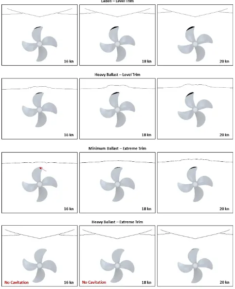
To post-process the cavitation development, an average cavitation volume over one propeller rotation was calculated and plotted for comparison. In addition, the wake angle range over which cavitation appeared was computed along with the amount of sheet cavitation as percentage of propeller blade area. A visual comparison of propeller cavitation was also performed by extracting a front-view image of the propeller at an instance of maximum cavitation volume.

4 SIMULATION RESULTS

At the end of each simulation run, further data describing the cavitation pattern and volume were extracted automatically and again, post-processed and compared in order to evaluate the influence of extreme trim on propeller cavitation. In addition, the influence of cavitation on the propeller performance was assessed. Results will be presented in a comparative manner, labelling each loading conditions with #1 - #4 according to Table1.

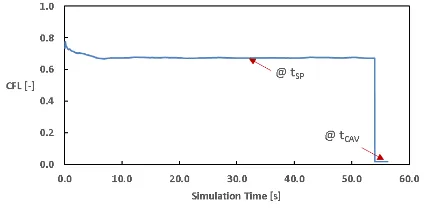
During each simulation run, the accuracy of the numerical solver was monitored by recording a time and cell value history of the Courant number (𝐶𝐹𝐿) and the 𝑌+ on the hull and the propeller respectively. For further information about the theoretical background of both 𝐶𝐹𝐿 and 𝑌+ the reader can refer to (ITTC, 2014).

Figure 5 Time History of CFL Number on and near LNG Carrier Hull

Figure 5 shows the average Courant number in the cells on and near the LNG Carrier hull for fully laden conditions at 14 knots full-scale speed. For both, the large time step (see Eq. 11) and the small time step (see Eq. 12) a value of 𝐶𝐹𝐿 < 1 was computed. Since the time step was coupled to the ship speed a similar CFL time history was recorded for each speed and loading condition. The same velocity-dependent approach was used for the generation of the near wall mesh which determined the 𝑌+ (see Figure 66).

Figure 6 Average Y+ on the LNG Carrier Hull

For monitoring the 𝐶𝐹𝐿 and the 𝑌+ on the propeller blades, a more detailed histogram plot was chosen to track the values per number of cells.

Figure 7 Histogram of Courant Number in Cells of Propeller Blades

Whereas the flow within the majority of cells, i.e. 80%, on the propeller blades was solved with a 𝐶𝐹𝐿 < 1, 20% of the cells were solved with values of 1 < 𝐶𝐹𝐿 < 30. Those cells were mainly distributed along the blade leading edge where high flow velocities appeared.

Figure 8 Histogram of Y+ in Cells of Propeller Blades

Approximately the same distribution of cells (80%/20%) was found for the 𝑌+< 2 and 2 < 𝑌+< 6.

4.1 Performance at Self-Propulsion Point

In effective (self-propulsion) operating conditions, i.e. the propeller rotates behind the ship hull, in order to operate at the self-propulsion point, the generated thrust by the propeller is higher than the resistance of the bare ship hull in nominal conditions. The additional resistance induced by the propeller originates from an increase of flow velocities at the aftbody of the hull – resulting in an increase in frictional resistance, and a decrease of the pressure at the aftbody – resulting in an increase in inviscid resistance. This phenomena can be expressed by the thrust deduction factor, which relates the nominal resistance to the thrust created by the propeller in effective conditions. (Bertram, 2000b)

If results from nominal resistance simulations/tests and self-propulsion simulations/tests are available, as for the present study, the thrust deduction factor can be calculated as shown in Eq. 17 (Carlton, 2011).

𝑡 =𝑇 + 𝐹0− 𝑅𝑇,𝑛𝑜𝑚𝑖𝑛𝑎𝑙

Figure 9 Thrust Deduction Fraction

Compared to values for thrust deduction factors that can be calculated from empirical equations for this type of single-screw ship (for empirical equations see (Carlton, 2011)), the above values are relatively high for lower ship speeds and reasonable for higher ship speeds. Overall, the interaction between propeller and ship hull improves at higher ship speeds. In particular, for the level trim conditions #1 and #2, the performance decreases at heavy ballast draft (#2) as the propeller operates close to the free surface. The extreme trim conditions #3 and #4 show a better performance compared to the level trim conditions. This can be explained by the much smaller imprint of the ship hull on the wake field (i.e. wake fraction), hence a more uniform propeller inflow (see reader may refer to (Maasch et al., 2017) for details). Since the ship power delivered to the propeller is calculated from propeller 𝑟𝑝𝑠 and torque, it is worthwhile to present those quantities in a comparative manner, too. Hence, Figure 10 and Figure 11 compare 𝑟𝑝𝑠 and torque for the calculated loading conditions. The propeller 𝑟𝑝𝑠 was mainly driven by the ship speed and displacement as for low speed and low displacement a low 𝑟𝑝𝑠 was computed. Consequently, the fully laden condition #1 showed the highest 𝑟𝑝𝑠, followed by the heavy ballast loading level trim condition #2 and the heavy ballast extreme trim condition #3. For the minimum ballast extreme trim condition #4 the propeller operated with the lowest 𝑟𝑝𝑠 due to largely reduced ship displacement.

Figure 10 Propeller RPS

The propeller torque, shown below in Figure 11, reflects the quality of the operating conditions for the propeller at more detail and somewhat independent of small differences in ship displacement. It is evident that the load on the propeller largely reduces in extreme trim conditions. However, for both, the level trim conditions #1 and #2 and the extreme trim conditions #3 and #4, the torque values

are close with almost no difference between #3 and #4. This demonstrates that the propeller works efficiently in extreme trim conditions.

Figure 11 Propeller Torque

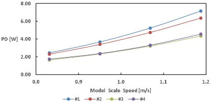
Following Eq. 6, both propeller 𝑟𝑝𝑠 and propeller torque yield the power delivered to the propeller. As presented in Figure 12, the required power is similar to the trend of the propeller torque. Since the propeller showed a good performance in heavy ballast extreme trim conditions #4, there is only a small difference to the minimum ballast extreme trim condition #3, despite the higher displacement.

Figure 12 Power Delivered to the Propeller

This phenomena can be explained by the increased submergence of the aftship which allowed the propeller to work in a more favorable flow environment.

4.2 Propeller Cavitation

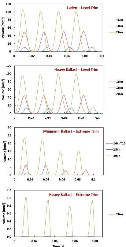
speeds. At heavy ballast level trim conditions (#2) the lower draft caused a slightly higher cavitation volume, despite the reduced propeller rps. For the minimum ballast extreme trim condition (#3), hardly any cavitation was detectable when checking the vapor volume visually during the simulation run. However, the solver computed cavitation volume, here presented as ten times as much (see 3rd chart in Figure 13) as actually recorded. For the heavy ballast extreme trim loading condition (#4), no cavitation was computed for the three lower speeds. Only at the speed corresponding to 20 knots full-scale, cavitation occurred.

Figure 13 Transient Cavitation Volume per Propeller Rotation

From the transient recordings of the cavitation volume, an average was calculated, allowing to compare each speed and loading condition with less detail (see Figure ).

Figure 14 Average Cavitation Volume per Propeller Rotation

Due to the low draft at condition #2 the propeller operated very close to the water surface, hence producing a similar average cavitation volume as the LNG Carrier operating in fully laden conditions. This can also be seen in Figure 14. In extreme trim conditions at a minimum ballast, only little cavitation volume occurred.

Finally, the percentage of sheet cavitation on the propeller blade area was calculated as shown in Figure 15. Using this quantity, one can estimate if and by how much the thrust generated by the propeller breaks down due to cavitation. If the thrust breaks down due to cavitation, one would need to operate at higher propeller 𝑟𝑝𝑠 since the decreased thrust leads to a higher power consumption for a constant speed (Lewis, 1988).

Figure 15 Area of Sheet Cavitation as Percentage of Propeller Blade Area

5 CONCLUSION AND OUTLOOK

Within the presented study, numerical self-propulsion simulations including the prediction of propeller cavitation for an LNG Carrier geometry at model scale were performed. Four loading conditions were computed, two at level trim and two at an extreme bow-up trim angle. This was done to show how the self-propulsion performance of the ship improves when operated at an extreme trim angle.

The presented simulation setup, which was largely automated by coupling commercial software tools suitable to perform a marine CFD study, allowed to pre-process, run and post-process the simulations with only little interaction of the user compared to an approach where repeatable steps in the setup would have been executed manually. Thus, a set of 16 numerical simulations were prepared, executed and assessed in a short period of time.

Two objectives were investigated within this study, the effect of the Extreme Trim Concept on the power delivered to the propeller and on the propeller cavitation.

It was shown that by operating the LNG Carrier at an extreme bow up trim angle, the power consumption was reduced by around 25%. This substantial reduction was reached by reducing the ship displacement while at the same time keeping a favorable inflow to the operating propeller. Fortunately, the heavy ballast extreme trim loading condition showed similar improvements in the required power reduction as the extreme trim operation condition at minimum ballast. Thus, due to the higher displacement, it is likely that an improved ship stability would be reached when operating in waves.

Due to the propeller operating at lower 𝑟𝑝𝑠 in extreme trim conditions compared to level trim, the propeller cavitation was reduced substantially, too. At level trim conditions, the propeller cavitated at speeds corresponding to 16, 18 and 20 knots full-scale. At the most favorable loading condition (heavy ballast extreme trim), only at 20 knots cavitation was detectable. For all simulated cases the cavitation did not cause a thrust breakdown.

In order to extend the work done within this project, the LNG Carrier performance should be investigated at higher speeds with a more refined numerical mesh in order to capture more details of cavitation. In addition, the influence of the Extreme Trim Concept on both the seakeeping performance and the ship stability would need to be assessed, too.

ACKNOWLEDGEMENT

This research has been funded by the Engineering and Physical Research Council (EPSRC) through the project, “Shipping in Changing Climates. All supports are greatly appreciated. EPSRC grant no. EP/K039253/1.

Results were obtained using the EPSRC funded ARCHIE-WeSt High Performance Computer (www.archie-west.ac.uk). EPSRC grant no. EP/K000586/1. The authors would like to further acknowledge Lloyds Register and SHELL as sponsors of this study.

REFERENCES

BERTRAM, V. 2000a. Practical Ship Hydrodynamics. 1.4 Numerical approaches (computational fluid dynamics) Butterworth-Heinemann.

BERTRAM, V. 2000b. Practical Ship Hydrodynamics. 3.1 Resistance and propulsion concepts. Butterworth-Heinemann.

CARLTON, J. S. 2011. Marine Propellers and Propulsion. Chapter 12 - Ship Resistance and Propulsion. Butterworth-Heinemann.

DAY, S., CLELLAND, D. & TURAN, O. 2010. Tests of LNG Carrier in Calm Water and Waves - Summary of Results. University of Strathclyde.

HOLLENBACH, U., KLUG, H. & MEWIS, F. 2007. Container Vessels – Potential for Improvements in Hydrodynamic Performance. 10th International Symposium on Practical Design of Ships and Other Floating Structures. Design of Ships and Other Floating Structures: American Buero of Shipping.

ITTC 2014. ITTC – Recommended Procedures and Guidelines. 7.5-03-02-03 Practical Guidelines for Ship CFD Applications.

ITTC 2017a. ITTC – Recommended Procedures and Guidelines. 7.5-02-03-01.1 Propulsion/Bollard Pull Test.

ITTC 2017b. ITTC – Recommended Procedures and Guidelines. 7.5-02-02-01 Resistance Test.

LEWIS, E. W. 1988. Principles of Naval Architecture Second Revision. In: LEWIS, E. W. (ed.) Volume II - Resistance, Propulsion and Vibration. The Society of Naval Architects and Marine Engineers.

MAASCH, M., TURAN, O., KHORASANCHI, M. & FANG, I. 2017. Calm water resistance and self propulsion simulations including cavitation for an LNG carrier in extreme trim conditions. Shipping in Changing Climates SCC 2017. London.

MEWIS, F. & HOLLENBACH, U. 2007. Hydrodynamic Measures for Reducing Energy Consumption during Ship Operation. STG Sprechtag „Möglichkeiten der Energieeinsparung im Schiffsbetrieb“. Hamburg.

PERIC, M. & FERGUSON, S. 2005. The advantage of

polyhedral meshes. Available:

https://pdfs.semanticscholar.org/51ae/90047ab44f538491 96878bfec4232b291d1c.pdf.

REICHEL, M., MINCHEV, A. & LARSEN, N. L. 2014. Trim Optimisation - Theory and Practice. 20th International Conference on Hydrodynamics in Ship Design and Operation. Wrocław: FORCE Technology. SCHNERR, G. H. & SAUER, J. 2001. Physical and Numerical Modeling of Unsteady Cavitation Dynamics. ICMF-2001, 4th International Conference on Multiphase Flow. New Orleans, USA.

SIEMENS 2017b. STAR-CCM+ Documentation. Using the Volume Of Fluid (VOF) Multiphase Model.