City, University of London Institutional Repository
Citation
: Brain, M. ORCID: 0000-0003-4216-7151, Niemetz, A., Preiner, M., Reynolds, A.,
Barrett, C. and Tinelli, C. (2019). Invertibility Conditions for Floating-Point Formulae. In:
Computer Aided Verification. CAV 2019. Lecture Notes in Computer Science, 11562. (pp.
116-136). Cham: Springer. ISBN 978-3-030-25542-8
This is the published version of the paper.
This version of the publication may differ from the final published
version.
Permanent repository link:
http://openaccess.city.ac.uk/id/eprint/22749/
Link to published version
:
Copyright and reuse:
City Research Online aims to make research
outputs of City, University of London available to a wider audience.
Copyright and Moral Rights remain with the author(s) and/or copyright
holders. URLs from City Research Online may be freely distributed and
linked to.
Formulas
Martin Brain3,4 , Aina Niemetz1 , Mathias Preiner1(B) ,
Andrew Reynolds2 , Clark Barrett1 , and Cesare Tinelli2
1 Stanford University, Stanford, USA
preiner@cs.stanford.edu
2 The University of Iowa, Iowa City, USA 3 University of Oxford, Oxford, UK 4 City, University of London, London, UK
Abstract. Automated reasoning procedures are essential for a number of applications that involve bit-exact floating-point computations. This paper presents conditions that characterize when a variable in a floating-point constraint has a solution, which we call invertibility conditions. We describe a novel workflow that combines human interaction and a syntax-guided synthesis (SyGuS) solver that was used for discovering these con-ditions. We verify our conditions for several floating-point formats. One implication of this result is that a fragment of floating-point arithmetic admits compact quantifier elimination. We implement our invertibility conditions in a prototype extension of our solver CVC4, showing their usefulness for solving quantified constraints over floating-points.
1
Introduction
Satisfiability Modulo Theories (SMT) formulas including either the theory of floating-point numbers [12] or universal quantifiers [24,32] are widely regarded as some of the hardest to solve. Problems that combine universal quantification over floating-points are rare—experience to date has suggested they are hard for solvers and would-be users should either give up or develop their own incomplete techniques. However, progress in theory solvers for floating-point [11] and the use of expression synthesis for handling universal quantifiers [27,29] suggest that these problems may not be entirely out of reach after all, which could potentially impact a number of interesting applications.
This paper makes substantial progress towards a scalable approach for solv-ing quantified floatsolv-ing-point constraints directly in an SMT solver. Developsolv-ing procedures for quantified floating-points requires considerable effort, both foun-dationally and in practice. We focus primarily on establishing a foundation for lifting to quantified floating-point formulas a procedure for solving quantified bit-vector formulas by Niemetz et al. [26]. That procedure relies on so-called
This work was supported in part by DARPA (award no. FA8650-18-2-7861), ONR (award no. N68335-17-C-0558) and NSF (award no. 1656926).
c
The Author(s) 2019
I. Dillig and S. Tasiran (Eds.): CAV 2019, LNCS 11562, pp. 116–136, 2019.
invertibility conditions, intuitively, formulas that state under which conditions an argument of a given operator and predicate in an equation has a solution. Building on this concept and a state-of-the-art expression synthesis engine [29], we generate invertibility conditions for a majority of operators and predicates in the theory of point numbers. In the context of quantifier-free floating-point formulas, floating-floating-point invertibility conditions may enable us to lift the propagation-based local search approach for bit-vectors in [25] to the theory of floating-point numbers.
This work demonstrates that invertibility conditions exist and show promise for solving quantified floating-point constraints. More specifically, it makes the following contributions:
– In Sect.3, we present invertibility conditions for the majority of operators and predicates in the SMT-LIB standard theory of floating-point numbers. – In Sect.4, we present a custom methodology based on syntax-guided synthesis
and decision tree learning that we developed for the purpose of synthesizing the invertibility conditions presented here.
– In Sect.5, we present a quantifier elimination procedure for a fragment of the theory that is based on invertibility conditions, and give experimental evidence of its potential, based on quantified floating-point problems coming from a verification application.
Related Work. To our knowledge, no previous work specifically discusses tech-niques for solving universally quantified floating-point formulas. Brain et al. [11] provide a comprehensive review of decision procedures for quantifier-free bit-exact floating-point using both SMT-based as well as other approaches. They identify four groups of techniques: bit-blasting approaches that use floating-point circuits to generate bit-vector formulas [13,16,20,33], interval techniques that use partitioning and interval propagation [10,22,23,31], optimization and numer-ical approaches that work with complete valuations [4,7,18,21], and axiomatic techniques that use partial or total axiomatizations of the theory of floating-point numbers in other theories such as real arithmetic [14,15].
On the other hand, approaches for universal quantification have been devel-oped in modern SMT solvers that target other background theories, includ-ing linear arithmetic [8,17,29] and bit-vectors [26,27,32]. At a high level, these approaches use model-based refinement loops that lazily add instances of univer-sal quantifiers until they reach a conflict at the quantifier-free level, or otherwise saturate with a model.
2
Preliminaries
We assume the usual notions and terminology of many-sorted first-order logic with equality (denoted by≈). LetΣbe asignatureconsisting of a setΣsof sort symbols and a setΣfof interpreted (and sorted) function symbols. Each function symbolf
has a sortτ1×...×τn→τ, with arityn≥0 andτ1, ..., τn, τ ∈Σs. We assume that
We further assume the usual definition of well-sorted terms, literals, and (quanti-fied) formulas with variables and symbols fromΣ, and refer to them asΣ-terms,
Σ-atoms, and so on. For aΣ-term orΣ-formulae, we denote thefree variables ofe(defined as usual) asF V(e) and usee[x] to denote that the variablexoccurs free ine. We writee[t] for the term or formula obtained fromeby replacing each occurrence ofxinebyt.
AtheoryT is a pair (Σ, I), whereΣis a signature andIis a non-empty class ofΣ-interpretations (themodelsofT) that is closed under variable reassignment, i.e., every Σ-interpretation that only differs from an I ∈I in how it interprets variables is also inI. AΣ-formulaϕisT-satisfiable (resp.T-unsatisfiable) if it is satisfied by some (resp. no) interpretation inI; it isT-validif it is satisfied by all interpretations inI. We will sometimes omitTwhen the theory is understood from context.
We briefly recap the terminology and notation of Brain et al. [12] which defines an SMT-LIB theoryTFP of floating-point numbers based on the IEEE-754 2008 standard [3]. The signature of TFP includes a parametric family of sorts Fε,σ where ε and σ are integers greater than or equal to 2 giving the number of bits used to store the exponent e and significand s, respectively. Each of these sorts contains five kinds of constants: normal numbers of the form 1.s∗2e, subnormal numbers of the form 0.s∗2−2σ−1−1, two zeros (+0 and−0), two infinities (+∞ and −∞) and a single not-a-number (NaN). We assume a map vε,σ for each sort, which maps these constants to their value in the set R∗=R∪ {+∞,−∞,NaN}. The theory also provides a rounding-mode sortRM, which contains five elements{RNE,RNA,RTP,RTN,RTZ}.
Table1 lists all considered operators and predicate symbols of theory TFP. The theory contains a full set of arithmetic operations{|. . .|,+,−,·,÷,√,max,
min}as well asrem(remainder),rti(round to integral) andfma(combined mul-tiply and add with just one rounding). The precise semantics of these operators is given in [12] and follows the same general pattern: vε,σ is used to project the arguments to R∗, the normal arithmetic is performed inR∗, then the rounding mode and the result are used to select one of the adjoints of vε,σ to convert the result back toFε,σ. Note that the full theory in [12] includes several addi-tional operators which we omit from discussion here, such as floating-point min-imum/maximum, equality with floating-point semantics (fp.eq), and conversions between sorts.
TheoryTFP further defines a set of ordering predicates {<, >,≤,≥} and a set of classification predicates{isNorm,isSub,isInf,isZero,isNaN,isNeg,isPos}. In the following, we denote the rounding mode of an operation above the operator symbol, e.g.,aRTZ+baddsaandband rounds the result towards zero. We use the infix operator style for isInf (. . . ≈ ±∞), isZero (. . . ≈ ±0), andisNaN (. . . ≈
NaN) for conciseness. We further use minn/maxn and mins/maxs for
3
Invertibility Conditions for Floating-Point Formulas
In this section, we adapt the concept of invertibility conditions introduced by Niemetz et al. in [26] to our theoryTFP. Intuitively, an invertibility conditionφc
for a literall[x] is the exact condition under whichl[x] has a solution forx, i.e.,
φc is equivalent to ∃x. l[x] inTFP.
Definition 1 (Floating-Point Invertibility Condition).Letl[x] be aΣF P-literal. A quantifier-free ΣF P-formula φc is an invertibility condition for x in l[x] if
x∈F V(φc) andφc⇔ ∃x. l[x] is TFP -valid.
As a simple example of an invertibility condition, given literal |x| ≈ t where
|x| denotes the absolute value of x, a solution for x exists if and only if t is not negative, i.e., if ¬isNeg(t) holds. We introduce additional terminology for the sake of the discussion. We define thedimension of an invertibility condition problem ∃x. l[x] as the number of free variables it contains. For example, if s
andtare variables, then the dimension of∃x. x+s≈tis two, the dimension of
∃x.isZero(x+s) is one, and the dimension of∃x.isZero(|x|) is zero. A literall[x] isfully invertibleif its invertibility condition is. A termeis an (unconditional) inverse forx in l[x] if l[e] is equivalent to . For example, the literal−x≈ t
is fully invertible and −t is an inverse for x in this literal. We say that e is a conditional inverse forl[x] ifl[e] is an invertibility condition for l[x].
[image:5.439.68.388.448.574.2]Our primary goal in this work is to establish invertibility conditions for all floating-point constraints that contain exactly one operator and one predicate. These conditions collectively suffice to characterize when any literal l[x] con-taining exactly one occurrence ofx, the variable to solve for, has a solution. In total, we were able to establish 167 out of 188 invertibility conditions (count-ing commutative cases only once) us(count-ing a syntax-guided synthesis framework which we describe in more detail in Sect.4. In this section, we present a subset of these invertibility conditions, highlighting the most interesting cases where
Table 1.Considered floating-point predicates/operators, with SMT-LIB 2 syntax.
Symbol SMT-LIB syntax Sort isNorm,isSub fp.isNormal, fp.isSubnormal Fε,σ→Bool isPos,isNeg fp.isPositive, fp.isNegative Fε,σ→Bool isInf,isNaN,isZero fp.isInfinite, fp.isNaN, fp.isZero Fε,σ→Bool
≈,<,>,≤,≥ =, fp.lt, fp.gt, fp.leq, fp.geq Fε,σ×Fε,σ→Bool
|. . .|,− fp.abs, fp.neg Fε,σ→Fε,σ
rem fp.rem Fε,σ×Fε,σ→Fε,σ √,rti fp.sqrt, fp.roundToIntegral RM×Fε,σ→Fε,σ
we succeeded (or failed) to establish an invertibility condition. Due to space restrictions, we omit the conditions for the remaining cases.1
Table 2.Invertibility conditions for floating-point operators (excl.fma) with≈. Literal Invertibility condition
x+R s≈t t≈(tRTP−s)+R s∨t≈(tRTN−s)+Rs∨s≈t
x−R s≈t t≈(sRTP+t)−R s∨t≈(sRTN+t)−Rs∨(s≈t∧s≈ ±∞ ∧t≈ ±∞) s−R x≈t t≈s+ (R tRTP−s)∨t≈s+ (R tRTN−s)∨s≈t
xR·s≈t t≈(tRTP÷s)R·s∨t≈(tRTN÷s)R·s∨(s≈ ±∞ ∧t≈ ±∞)∨(s≈ ±0∧t≈ ±0) x÷R s≈t t≈(sRTP· t)÷R s∨t≈(sRTN· t)÷Rs∨(s≈ ±∞ ∧t≈ ±0)∨(t≈ ±∞ ∧s≈ ±0) s÷R x≈t t≈s÷R (sRTP÷t)∨t≈s÷R (sRTN÷t)∨(s≈ ±∞ ∧t≈ ±∞)∨(s≈ ±0∧t≈ ±0) xrems≈t t≈trems
sremx≈t ? R
√x≈t t≈R
(tRTP· t)∨t≈R
(tRTN· t)∨t≈ ±0 |x| ≈t ¬isNeg(t)
−x≈t R
rti(x)≈t t≈rtiR(t)
Table2 lists the invertibility conditions for equality with the operators
{+,−,·,÷,rem,√,|. . .|,−,rti}, parameterized over a rounding modeR (one of
RNE,RNA,RTP,RTN, or RTZ). Note that operators{+,·}and the multiplica-tive step offmaare commutative, and thus the invertibility conditions for both variants are identical.
Each of the first six invertibility conditions in this table follows a pattern. The first two disjuncts are instances of the literal to solve for, where a term involving rounding modes RTP and RTN is substituted for x. These disjuncts are then followed by disjuncts for handling special cases for infinity and zero. From the structure of these conditions, e.g., for +, we can derive the insight that if there is a solution forxin the equationx+R s≈tand we are not in a corner case where
s=t, then eithertRTP−sortRTN−smust be a solution. Based on extensive runs of our syntax-guided synthesis procedure, we believe this condition is close to having minimal term size. From this, we conclude that an efficient yet complete method for solvingx+R s≈tchecks whethert−srounding towards positive or negative is a solution in the non-trivial case when s and t are disequal, and otherwise concludes that no solution exists. A similar insight can be derived for the other invertibility conditions of this form.
We found that t is a conditional inverse for the case of R
rti(x)≈t and
xrems≈t, that is, substituting t for x is an invertibility condition. For the latter, we discovered an alternative invertibility condition:
|tRTP+t| ≤ |s| ∨ |tRTN+t| ≤ |s| ∨ite(t≈ ±0, s≈ ±0, t≈ ±∞) (1)
In contrast to the condition from Table2, this version does not involve rem. It follows that certain applications of floating-point remainder, including those whose first argument is an unconstrained variable, can be eliminated based on this equivalence. Interestingly, for sremx≈t, we did not succeed in finding an invertibility condition. This case appears to not admit a concise solution; we discuss further details below.
Table3gives the invertibility conditions for≥. Since these constraints admit more solutions, they typically have simpler invertibility conditions. In particular, with the exception ofrem, all conditions only involve floating-point classifiers.
When considering literals with predicates, the invertibility conditions for cases involving x+s and s−x are identical for every predicate and rounding mode. This is due to the fact that s−x is equivalent to s+ (−x), indepen-dent from the rounding mode. Thus, the negation of the inverse value of xfor an equation involving x+s is the inverse value of xfor an equation involving
s−x. Similarly, the invertibility conditions for x·s and s÷x over predicates
[image:7.439.67.379.411.588.2]{<,≤, >,≥,isInf,isNaN,isNeg,isZero} are identical for all rounding modes. For all predicates except {≈,isNorm,isSub}, the invertibility conditions for operators {+,−,÷,·}contain floating-point classifiers only. All of these condi-tions are also independent from the rounding mode. Similarly, for operatorfma over predicates {isInf,isNaN,isNeg,isPos}, the invertibility conditions contain
Table 3.Invertibility conditions for floating-point operators (excl.fma) with≥.
Literal Invertibility condition
x+Rs≥t (isPos(s)∨ite(s≈ ±∞,(t≈ ±∞ ∧isNeg(t)),isNeg(s)))∧t≈NaN
x−Rs≥t ite(isNeg(s), t≈NaN,ite(s≈ ±∞,(t≈ ±∞ ∧isNeg(t)),(isPos(s)∧t≈NaN)))
s−Rx≥t (isPos(s)∨ite(s≈ ±∞,(t≈ ±∞ ∧isNeg(t)),isNeg(s)))∧t≈NaN
xR·s≥t (isNeg(t)∨t≈ ±0∨s≈ ±0)∧s≈NaN∧t≈NaN
x÷Rs≥t (isNeg(t)∨t≈ ±0∨s≈ ±∞)∧s≈NaN∧t≈NaN
s÷Rx≥t (isNeg(t)∨t≈ ±0∨s≈ ±0)∧s≈NaN∧t≈NaN
xrems≥t ite(isNeg(t), s≈NaN,(|tRNE+t| ≤ |s| ∧t≈ ±∞))∧s≈ ±0
sremx≥t ?
R
√
x≥t t≈NaN |x| ≥t t≈NaN −x≥t t≈NaN
R
only floating-point classifiers. All of these conditions except forisNeg(fma(x, s, t)) andisPos(fma(x, s, t)) are also independent from the rounding mode.
For all floating-point operators with predicateisNaN, the invertibility condi-tion is , i.e., an inverse value for xalways exists. This is due to the fact that every floating-point operator returns NaN if one of its operands isNaN, hence
NaNcan be picked as an inverse value of x. Conversely, we identified four cases for which the invertibility condition is⊥, i.e., an inverse value forxnever exists. These four cases areisNeg(|x|),isInf(xrems),isInf(sremx), andisSub(rti(x)). For the first three cases, it is obvious why no inverse value exists. The intuition for
isSub(rti(x)) is that integers are not subnormal, and as a result ifxis rounded to an integer it can never be a subnormal number. All of these cases can be easily implemented as rewrite rules in an SMT solver.
For operator fma, the invertibility conditions over predicates {isInf,isNaN,
isNeg,isPos} contain floating-point classifiers only. For predicate isZero, the invertibility conditions are more involved. Equations (2) and (3) show the invert-ibility conditions for isZero(fma(x, s, t)) andisZero(fma(s, t, x)) for all rounding modesR.
R
fma(−(tRTP÷s), s, t)≈±0∨fmaR (−(tRTN÷s), s, t)≈±0∨(s≈±0∧t≈±0) (2)
R
fma(s, t,−(sRTP· t))≈±0∨fmaR (s, t,−(sRTN· t))≈±0 (3)
These two invertibility conditions contain case splits similar to those in Table2and
indicate that, e.g.,−tRTP÷sis an inverse value forxwhen R
fma(−(tRTP÷s), s, t)≈±0 holds.
As we will describe in Sect.4, an important aspect of synthesizing these invertibility conditions was considering their visualizations. This helped us deter-mine which invertibility conditions were relatively simple and which exhibited complex behavior.
s
t
(a)x+s≈t
s
(b)x·s≈t
s
(c)x÷s≈t
s
[image:8.439.43.385.425.540.2](d)s÷x≈t
s t
(a)xrems≈t
s t
[image:9.439.125.330.56.171.2](b)sremx≈t
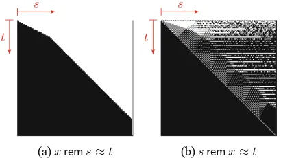
Fig. 2.Invertibility conditions forremover≈forF3,5.
Figure1 shows the visualizations of the invertibility conditions for operators
{+,·,÷}over≈from Table2for sortF3,5with rounding modeRNE(each of the
literals is two-dimensional). We use 227×227 pixel maps over all possible values ofsandt, where the pixel at point (s, t) is white if the invertibility condition is true, and black if it is false.2 The values ofsare plotted on the horizontal axis
and the values of t are plotted on the vertical axis. The leftmost two columns (resp. topmost two rows) give the value of the invertibility condition fors=±0 (resp.t=±0); the rightmost column (resp. bottom row) gives its value forNaN; the next two columns left of (resp. next two rows on top of)NaN give its value for ±∞; the remainder plots the values of the subnormal and normal values of
s andt, left-to-right (resp. top-to-bottom) in increasing order of their absolute value, alternating between positive and negative values. These visualizations give an intuition of the complexity of the behavior of invertibility conditions, which is a consequence of the complex semantics of floating-point operations.
Figure2 gives the invertibility condition visualizations for remainder over
≈ with sort F3,5 and rounding mode RNE. The visualization on the left hand
shows that solving forxas the first argument is relatively easy. It suggests that an invertibility condition for this case involves a linear inequality relating the absolute values ofsandt, which we were able to derive in Eq. (1). Solving forx
as the second argument, on the other hand, is much more difficult, as indicated by the right picture, which has a significantly more complex structure. We con-jecture that no simple solution exists for the latter problem. The visualization of the invertibility condition gives some of the intuition for this: the diagonal divide is caused by the fact that outputtwill always have a smaller absolute value than the input s. The top-left corner represents subnormal/subnormal computation, this acts as fixed-point and behaves differently from the rest of the function. The stepped blocks along the diagonal occur whensandthave the same expo-nent and thus the pattern is similar to the invertibility condition for + shown in Fig.1. Portions right of the main diagonal appear to exhibit random behavior.
2 Notice that we consider all possible (2σ−1−1)∗2NaNvalues ofT
s
t
(a)xrems > t
s
(b)xrems≥t
s
(c)sremx > t
s
[image:10.439.49.384.53.169.2](d)sremx≥t
Fig. 3.Invertibility conditions forremover inequalities forF3,5. s
t
(a)fma(x, s, t)≈ ±0
s
(b)fma(s, t, x)≈ ±0
s
(c)isSub(fma(x, s, t))
s
[image:10.439.41.384.209.314.2](d)isSub(fma(s, t, x))
Fig. 4.Invertibility conditions forfmaover{isZero,isSub}forF3,5and rnd. modeRNE.
We believe this is the result of repeated cancellations in the computation of the remainder for those values, which suggests a behavior that we believe is similar to the Blum-Blum-Shub random number generator [9].
For remainder with inequalities, we succeeded in determining invertibility conditions for ≤ and ≥ if x is the first argument. However, for xrems over
{<, >}, andsremxover{≥,≤, <, >} we did not. This is particularly surprising considering that the invertibility conditions for non-strict and strict inequalities are nearly identical (varying only by a handful of pixels), as shown in Fig.3. Note that for xas the first argument, all variations of the concise invertibility conditions for non-strict inequality we considered failed as solutions for the strict inequality. This behavior is representative of the many subtle corner cases we encountered while synthesizing these conditions.
4
Synthesis of Floating-Point Invertibility Conditions
Deriving invertibility conditions in TFP is a highly challenging task. We were unable to derive these conditions manually despite our substantial background knowledge of floating-point numbers. As a consequence, we developed a custom extension of the syntax-guided synthesis (SyGuS) paradigm [1] with the goal of finding invertibility conditions automatically, which resulted in the conditions from Sect.3. While the extension was optimized for this task, we stress that our techniques are theory-agnostic and can be used for synthesis problems over any finite domain. Our approach builds upon the SyGuS capabilities of the SMT solver CVC4 [5,29], which has recently been extended to support reasoning about the theory of floating-points [11]. We use the invertibility condition for floating-point addition with equality here as a running example.
Establishing an invertibility condition requires solving a synthesis problem with three levels of quantifier alternation. In particular, for floating-point addi-tion with equality, we are interested in finding a soluaddi-tion for predicate IC that satisfies the conjecture:
∃IC.∀s, t.(IC(s, t)⇔(∃x. x+R s≈t)) (4)
for some rounding mode R. In other words, this conjecture states that IC(s, t) holds exactly when there exists anxthat, when rounding the result of addingx
to s according to modeR, yieldst. Furthermore, we are interested in finding a solution forICthat holdsindependently of the format ofx, s, t. Note that SMT solvers are not capable of reasoning about constraints that are parametric in the floating-point format. To address this challenge, following the methodology from previous work [26], our strategy for establishing (general) invertibility conditions first solves the synthesis conjecture for a fixed format Fε,σ, and subsequently checks whether that solution also holds for other formats. The choice of the number of exponent bitsεand significand bitsσin Fε,σ balances two criteria:
1. ε,σshould be large enough to exercise many (or all) of the behaviors of the operators and relations in our synthesis conjecture,
2. ε,σshould be small enough for the synthesis problem to be tractable.
Assume we have chosen to synthesize the invertibility condition for conjec-ture (4) for format F3,5 and rounding mode RNE. Notice that current SyGuS
solvers [2,29] support only two levels of quantifier alternation. However, we can expand the innermost quantifier in this conjecture to obtain the conjecture:
∃IC.∀st.(IC(s, t)⇔(
226
i=0
iRNE+s≈t)) (5)
where for simplicity of notation we use i = 0, . . . ,226 to denote the values of F3,5. This methodology was also used in Niemetz et al. [26], where invertibility
conditions for bit-vector operators were synthesized for bit-width 4 by giving the conjecture of the above form to an off-the-shelf SyGuS solver. In contrast to that work, we found that the synthesis conjecture above is too challenging to be solved efficiently by current state-of-the-art enumerative SyGuS solvers. The reason for this is twofold. First, the smallest viable floating-point format is 3 + 5 = 8 bits, which requires the body of (5) to have a significantly large number of disjuncts (227), which is more than ten times larger than the 16 disjuncts required when synthesizing 4-bit invertibility conditions for bit-vectors. Second, floating-point formulas are much harder to solve than bit-vector formulas, due to the complexity of their bit-blasted encodings. Thus, a significantly challenging satisfiability query must be solved for each candidate considered within the SyGuS solver.
To address the above challenges, we perform a more extreme preprocessing step on our synthesis conjecture, which computes the input/output behavior of the invertibility condition on all points in the domain ofsandt. In other words, we rephrase our synthesis conjecture as:
∃IC.
226
i=0 226
j=0
(IC(i, j)⇔ci,j) (6)
where eachci,jis a Boolean constant (eitheror⊥) determined by a quantifier-free satisfiability query. In particular, for each pair of floating-point values (i, j), constantci,jisifx+i≈jis satisfiable, and⊥if it is unsatisfiable. In practice, we represent the above conjecture as a 227×227 table, which we call the full I/O specification of invertibility condition IC. In our experiments, computing this table for most two-dimensional invertibility conditions of sortF3,5required
15 min (for 227∗227 = 51,529 quantifier-free queries), and 2 h for sort F4,5
(requiring 483∗483 = 233,289 queries). This process was accelerated by first applying random sampling over possible values ofxto quickly test if a query was satisfiable. For some operators, notably remainder, this required significantly more time than for others (up to a factor of 2). Due to the high cost of this preprocessing step, we generated a database with the full I/O specifications for all invertibility conditions from Sect.3 using a cluster of 50 nodes with Intel Xeon E5-2637 with 3.5 GHz and 32 GB memory, and then shared this database among multiple developers. Computing the full I/O specifications forF3,5,F4,5,
398.5 forF4,6). Despite the heavy cost of this step, it was crucial for accelerating
our framework for synthesizing invertibility conditions, described next.
PBE SyGuS Solver
Samples
SyGuS Grammar Side Condition
IC Candidate
User IC Problem
Verifier
Full I/O Spec solve
filter
[image:13.439.60.394.99.228.2]cex-guided sampling
Fig. 5.Architecture for synthesizing invertibility conditions for floating point formulas.
Figure5 summarizes our architecture for solving synthesis conjectures of the above form. The user first selects an invertibility condition problem to solve, where we assume the full I/O specification has been computed using the afore-mentioned techniques. At a high level, our architecture can be seen as an inter-active synthesis environment, where the user manages the interaction between two subprocedures:
1. a SyGuS solver with support for decision tree learning, and
2. a solution verifier storing the full I/O specification of the invertibility condition.
We use a counterexample-guided loop, where the SyGuS solver provides the solution verifier with candidate solutions, and the solution verifier provides the SyGuS solver with an evolving subset of sample points taken from the full I/O specification. These points correspond to counterexamples to failed candidate solutions, and are sampled in a uniformly random manner over the domain of our specification. To accelerate the speed at which our framework converges on a solution, we configure the solution verifier to generate multiple counterexample points (typically 10) for each iteration of the loop. The process terminates when the SyGuS solver generates a candidate solution that is correct for all points according to its full I/O specification.
a side condition, whose purpose is to focus on finding an invertibility condition that is correct for one of these subdomains. The side condition acts as a filter-ing mechanism on the counterexample points generated by the solution verifier. For example, given the side conditionisNorm(s)∧isNorm(t), the solution verifier checks candidate solutions generated by the SyGuS solver only against points (s, t) where both arguments are normal, and consequently only communicates counterexamples of this form to the SyGuS solver. The solution verifier may also be configured to establish that the current candidate solution generated by the SyGuS solver isconditionally correct, that is, it is true on all points in the domain that satisfy the side condition.
There are several advantages to the form of the synthesis conjecture in (6) that we exploit in our workflow. First, its structure makes it easy to divide the problem into sub-cases: our synthesis workflow at all times sends only a subset of the conjuncts of (6) for some (i, j) pairs. As a result, we do not burden the underlying SyGuS solver with the entire conjecture at once, which would not scale in practice. A second advantage is that it is in programming-by-examples (PBE) form, since it consists of a conjunction of concrete input-output pairs. As a consequence, specialized algorithms can be used by the SyGuS solver to generate solutions for (approximations of) our conjecture in a way that is highly scalable in practice. These techniques are broadly referred to as decision tree learning or unification algorithms. As a brief review (see Alur et al. [2] for a recent SyGuS-based approach), a decision tree learning algorithm is given as input a set of good examples c1 → , . . . , cn → and a set of bad examples
d1→ ⊥, . . . , dm→ ⊥. The goal of a decision tree algorithm is to find a predicate,
or classifier, that evaluates to true on all the good examples, and false on all the bad examples. In our context, a classifier is expressed as an if-then-else tree of Boolean sort. Sampling the space of conjecture (6) provides the decision tree algorithm with good and bad examples and the returned classifier is a candidate solution that we give to the solution verifier. The SyGuS solver of CVC4 uses a decision-tree learning algorithm, which we rely on in our workflow. Due to the scalability of this algorithm and the fact that only a small subset of our conjecture is considered at any given time, candidate solutions are typically generated by the SyGuS solver in our framework in a matter of seconds.
Another important aspect of the SyGuS solver in Fig.5is that it is configured to generate multiple solutions for the current set of sample points. Due to the way the SyGuS-based decision-tree learning algorithm works, these solutions tend to becomemore generalover the runtime of the solver. As a simple example (assuming exact integer arithmetic), say the solver is given input points (1,1)→
, (2,0)→ , (1,0)→ ⊥and (0,1)→ ⊥for (s, t). It enumerates predicates over
s andt, starting with simplest predicates first, say s≈0,t≈0,s≈1,y ≈1,
s+t > 1, and so on. After generating the first four predicates, it constructs the solution ite(s ≈ 1, t ≈ 1, t ≈ 0), which is a correct classifier for the given set of points. However, after generating the fifth predicate in this list, it returns
Since more general candidate solutions have a higher likelihood of being actual solutions in our experience, our workflow critically relies on the ability of users to manually terminate the synthesis procedure when they are satisfied with the last generated candidate. Our synthesis procedure logs a list of candidate solutions that satisfy the conjecture on the current set of sample points. When the user terminates the synthesis process, the solution verifier will check the last solution generated in this list. Users have the option to rearrange the elements of this list by hand, if they have an intuition that a specific candidate is more likely to be correct—and so should be tested first.
Experience. The first challenging invertibility condition we solved with our framework was addition with equality for rounding modeRNE. Initially, we used a generic grammar that contained the entire floating-point signature. As a first key step towards solving this problem, the synthesis procedure suggested the sin-gle literal t≈sRNE+ (tRNE−s) as candidate solution. Although counterexamples were found for this candidate, we noticed that it satisfied over 98% of the specification, and a visualization of its I/O behavior showed similar patterns to the invertibil-ity condition we were solving for. Based on these observations, we focused our grammar towards literals of this form. In particular, we used a function that takes two floating-pointsx, yand two rounding modesR1, R2 as arguments and
returnsxR1+(yR2−x) as a builtin symbol of our grammar. We refer to such a function as aresidual computation ofy, noting that its value is often approximatelyy. By including various functions for residual computations, we focused the effort of the synthesizer on more interesting predicates. The end solution involved multi-ple residual computations, as shown in Table2. Our initial solution was specific to the rounding modeRNE. After solving for several other rounding modes, we were able to construct a parametric solution that was correct for all rounding modes. In total, it took roughly three days of developer time to discover the generalized invertibility condition for addition with equality. Many of the sub-sequent invertibility conditions took a matter of hours, since by then we had a good intuition for the residual computations that were relevant for each case.
Invertibility conditions involvingrem, fma,isNorm, and isSubwere challeng-ing and required further customizations to the grammar, for instance to include constants that corresponded to the minimum and maximum normal and sub-normal values. Three-dimensional invertibility conditions (which in this work is limited to cases offmawith binary predicates) were especially challenging since the domain of their conjecture is a factor of 227 larger forF3,5than the others.
Following our strategy for solving the invertibility conditions for specific formats and rounding modes, in ongoing work we are investigating solving these cases by first solving the invertibility condition for a fixed value c for one of its free variables u. Solving a two-dimensional problem of this form with a solutionϕ
may suggest a generalization that works for all values ofuwhere all occurrences ofc inϕare replaced byu.
For instance, for some cases it was very easy to find invertibility conditions that held when bothsandtwere normal (resp., subnormal), but very difficult when
swas normal and twas subnormal or vice versa.
We also implemented a fully automated mode for the synthesis loop in Fig.5. However, in practice, it was more effective to tweak the generated solutions manually. The amount of user interaction was not prohibitively high in our experience.
Finally, we found that it was often helpful to visualize the input/output behavior of candidate solutions. In many cases, the difference between a candi-date solution and the desired behavior of the invertibility condition would reveal a required modification to the grammar or would suggest which parts of the domain of the conjecture to focus on.
4.1 Verifying Conditions for Multiple Formats and Rounding
Modes
We verified the correctness of all 167 invertibility conditions by checking them against their corresponding full I/O specification for floating-point formatsF3,5, F4,5, andF4,6and all rounding modes, which required 1.6 days of CPU time. This
is relatively cheap compared to computing the specifications, since checking is essentially constant evaluation of invertibility conditions for all possible input values. However, this quickly becomes infeasible with increasing precision, since the time required for computing the I/O specification roughly increases by a factor of 8 for each bit.
As a consequence, we generated quantified floating-point problems to verify the 167 invertibility conditions for formatsF3,5,F4,5,F4,6,F5,11(Float16),F8,24
(Float32), andF11,53(Float64) and all rounding modes. Each problem checks the
TFP-unsatisfiability of formula ¬(φc ⇔ ∃x. l[x]), where l[x] corresponds to the
[image:16.439.44.382.424.514.2]floating-point literal, andφc to its invertibility condition. In total, we generated
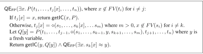
Fig. 6.Recursive procedureQEFPfor computing quantifier elimination forxin the unit
3786 problems (116∗5 + 513 for each floating-point format) and checked them
using CVC4 [5] (master 546bf686) and Z3 [16] (version 4.8.4).
We consider an invertibility condition to be verified for a floating-point format and rounding mode if at least one solver reports unsatisfiable. Given a CPU time limit of one hour and a memory limit of 8 GB for each solver/benchmark pair, we were able to verify 3577 (94.5%) invertibility conditions overall, with 99.2% of F3,5, 99.7% ofF4,5, 100% ofF4,6, 93.8% ofF5,11, 90.2% ofF8,24, and 84% ofF11,53.
This verification with CVC4 and Z3 required a total of 32 days of CPU time. All verification jobs were run on cluster nodes with Intel Xeon E5-2637 3.5 GHz and 32 GB memory.
5
Quantifier Elimination for Unit Linear Floating-Point
Formulas
Based on the invertibility conditions presented in Sect.3, we can define a quan-tifier elimination procedure for a restricted fragment of floating-point formulas. The procedure applies to unit linear formulas, that is, formulas of the form
∃x. P[x] where P is a ΣF P-literal containing exactly one occurrence of x. Figure6gives a quantifier elimination procedureQEFPfor unit linear floating-point formulas∃x. P[x]. We writegetIC(y, Q[y]) to indicate the invertibility con-dition foryin Q[y], which amounts to a table lookup for the appropriate condi-tion as given in Sect.3. Note that our procedure is currently a partial function because we do not have yet invertibility conditions for some unit linear formulas. The recursive procedure returns a conjunction of conditions based on the path on which xoccurs in P. Ifx occurs beneath multiple nested function applica-tions, a fresh variabley is introduced and used for referencing the intermediate result of the subterm we are currently solving for. We demonstrate this in the following example.
Example 2. Consider the unit linear formula ∃x.(xR·u)+R s ≥ t. Invoking the procedure QEFP on this input yields, after two recursive calls, the conjunction
getIC(y1, y1
R
+s≥t)∧getIC(y2, y2
R
·u≈y1)∧getIC(x, x≈y2)
where y1 and y2 are fresh variables. The third conjunct is trivially equivalent
to . This formula is quantifier-free and has the properties specified by the following theorem.
Theorem 1. Let ∃x. P be a unit linear formula and let I be a model of TFP. Then,Isatifies¬∃x. P if and only if there exists a modelJ ofTFP (constructible from I) that satisfies¬QEFP(∃x. P).
3 116 invertibility conditions from rounding mode dependent operators and 51
Niemetz et al. [26] present a similar algorithm for solving unit linear bit-vector literals. In that work, a counterexample-guided loop was devised that made use of Hilbert-choice expressions for representing quantifier instantiations. In contrast to that work, we provide here only a quantifier elimination procedure. Extending our techniques to a general quantifier instantiation strategy is the subject of ongoing work. We discuss our preliminary work in this direction in the next section.
6
Solving Quantified Floating-Point Formulas
We implemented a prototype extension of the SMT solver CVC4 that lever-ages the results of the previous section to determine the satisfiability of quanti-fied floating-point formulas. To handle quantiquanti-fied formulas, CVC4 uses a basic model-based instantiation loop (see, e.g., [30,32] for instantiation approaches for other theories). This technique maintains a quantifier-free set of constraints F
corresponding to instantiations of universally quantified formulas. It terminates with the response “unsatisfiable” ifF is unsatisfiable, and terminates with “sat-isfiable” if it can show that the given quantified formulas are satisfied by a model ofTFP that satisfiesF. ForTFP, the instantiations are substitutions of univer-sally quantified variables to concrete floating-point values, e.g.∀x. P(x)⇒P(0), which can be highly inefficient in the worst case for higher precision.
We extend this basic loop with a preprocessing pass that generates theory lemmas based on the invertibility conditions corresponding to literals of quanti-fied formulas∀x.P with exactly one occurrence ofx, as explained in the example below.
Example 3. Suppose the current set S of formulas contains a formula ϕof the form ∀x.¬((x·u) +s≥t∧Q(x)) where u,s andt are ground terms; then we add the following formula toS wherey1andy2are fresh (free) variables:
(getIC(y1, y1+s≥t)⇒y1+s≥t)∧(getIC(y2, y2·u≈y1)⇒y2·u≈y1)
The addition of this lemma is satisfiability preserving because, if the invertibility condition holds for y1+s≥t (resp.,y2·u≈y1), theny1 (resp.,y2) a solution
for that literal. We then add the instantiation lemma ϕ⇒ ¬((y2·u) +s≥t∧
Q(y2)). Althoughxis not necessarily linear in the body ofϕ, if both invertibility
conditions hold, then the combination of the above lemmas implies (y2·u)+s≥t, which together with the instantiation lemma allows the solver to infer that the remaining portion of the quantified formulaQcannot hold fory2. An inference
of this form may be more productive than enumerating the possible values ofx
in instantiations.
with equality and inequality. We implemented all cases of invertibility conditions for solving these cases. We extended our SMT solver CVC4 (GitHub master 5d248c36) with the above preprocessing pass (GitHub cav19fp 9b5acd74), and compared its performance with (configuration CVC4-ext) and without (configu-ration CVC4-base) the above preprocessing pass enabled to the SMT solver Z3 (version 4.8.4). All experiments were run on the same cluster mentioned earlier, with a memory limit of 8 GB and a 1800 s time limit. Overall, CVC4-base solved 35 benchmarks within the time limit (with no benchmarks uniquely solved com-pared to CVC4-ext), CVC4-ext solved 42 benchmarks (7 of these uniquely solved compared to the base version), and Z3 solved 56 benchmarks. While CVC4-ext solves significantly fewer benchmarks than Z3, we believe that the improvement over CVC4-base is indicative that our approach for invertibility conditions shows potential for solving quantified floating-point constraints in SMT solvers. A more comprehensive evaluation and implementation is left as future work.
7
Conclusion
We have presented invertibility conditions for a large subset of combinations of floating-point operators over floating-point predicates supported by SMT solvers. These conditions were found by a framework that utilizes syntax-guided synthe-sis solving, customized for our problem and developed over the course of this work. We have shown that invertibility conditions imply that a simple frag-ment of quantified floating-points admits compact quantifier elimination, and have given preliminary evidence that an SMT solver that partially leverages this technique can have a higher success rate on floating-point problems coming from a software verification application.
For future work, we plan to extend techniques for quantified and quantifier-free floating-point formulas to incorporate our findings, in particular to lift pre-vious quantifier instantiation approaches (e.g., [26]) and local search procedures (e.g., [25]) for bit-vectors to floating-points. We also plan to extend and use our synthesis framework for related challenging synthesis tasks, such as finding con-ditions under which more complex constraints have solutions, including those having multiple occurrences of a variable to solve for. Our synthesis framework is agnostic to theories and can be used for any sort with a small finite domain. It can thus be leveraged also for solutions to quantified bit-vector constraints. Finally, we would like to establish formal proofs of correctness of our invertibility conditions that are independent of floating-point formats.
References
2. Alur, R., Radhakrishna, A., Udupa, A.: Scaling enumerative program synthesis via divide and conquer. In: Legay, A., Margaria, T. (eds.) TACAS 2017. LNCS, vol. 10205, pp. 319–336. Springer, Heidelberg (2017). https://doi.org/10.1007/978-3-662-54577-5 18
3. IEEE Standards Association 754-2008 - IEEE standard for floating-point arith-metic (2008).https://ieeexplore.ieee.org/servlet/opac?punumber=4610933 4. Barr, E.T., Vo, T., Le, V., Su, Z.: Automatic detection of floating-point exceptions.
SIGPLAN Not.48(1), 549–560 (2013)
5. Barrett, C., et al.: CVC4. In: Gopalakrishnan, G., Qadeer, S. (eds.) CAV 2011. LNCS, vol. 6806, pp. 171–177. Springer, Heidelberg (2011). https://doi.org/10. 1007/978-3-642-22110-1 14
6. Barrett, C., Stump, A., Tinelli, C.: The satisfiability modulo theories library (SMT-LIB) (2010).www.SMT-LIB.org
7. Ben Khadra, M.A., Stoffel, D., Kunz, W.: goSAT: floating-point satisfiability as global optimization. In: FMCAD, pp. 11–14. IEEE (2017)
8. Bjørner, N., Janota, M.: Playing with quantified satisfaction. In: 20th International Conferences on Logic for Programming, Artificial Intelligence and Reasoning -Short Presentations, LPAR 2015, Suva, 24–28 November 2015, pp. 15–27 (2015) 9. Blum, L., Blum, M., Shub, M.: A simple unpredictable pseudo-random number
generator. SIAM J. Comput.15(2), 364–383 (1986)
10. Brain, M., Dsilva, V., Griggio, A., Haller, L., Kroening, D.: Deciding floating-point logic with abstract conflict driven clause learning. Formal Methods Syst. Des.45(2), 213–245 (2014)
11. Brain, M., Schanda, F., Sun, Y.: Building better bit-blasting for floating-point problems. In: Vojnar, T., Zhang, L. (eds.) TACAS 2019, Part I. LNCS, vol. 11427, pp. 79–98. Springer, Cham (2019).https://doi.org/10.1007/978-3-030-17462-0 5 12. Brain, M., Tinelli, C., R¨ummer, P., Wahl, T.: An automatable formal semantics
for IEEE-754 floating-point arithmetic. In: 22nd IEEE Symposium on Computer Arithmetic, ARITH 2015, Lyon, 22–24 June 2015, pp. 160–167. IEEE (2015) 13. Brillout, A., Kroening, D., Wahl, T.: Mixed abstractions for floating-point
arith-metic. In: FMCAD, pp. 69–76. IEEE (2009)
14. Conchon, S., Iguernlala, M., Ji, K., Melquiond, G., Fumex, C.: A three-tier strategy for reasoning about floating-point numbers in SMT. In: Majumdar, R., Kunˇcak, V. (eds.) CAV 2017. LNCS, vol. 10427, pp. 419–435. Springer, Cham (2017).https:// doi.org/10.1007/978-3-319-63390-9 22
15. Daumas, M., Melquiond, G.: Certification of bounds on expressions involving rounded operators. ACM Trans. Math. Softw.37(1), 1–20 (2010)
16. De Moura, L., Bjørner, N.: Z3: an efficient SMT solver. In: Ramakrishnan, C.R., Rehof, J. (eds.) TACAS 2008. LNCS, vol. 4963, pp. 337–340. Springer, Heidelberg (2008).https://doi.org/10.1007/978-3-540-78800-3 24
17. Dutertre, B.: Solving exists/forall problems in yices. In: Workshop on Satisfiability Modulo Theories (2015)
18. Fu, Z., Su, Z.: XSat: a fast floating-point satisfiability solver. In: Chaudhuri, S., Farzan, A. (eds.) CAV 2016. LNCS, vol. 9780, pp. 187–209. Springer, Cham (2016). https://doi.org/10.1007/978-3-319-41540-6 11
19. Heizmann, M., et al.: Ultimate automizer with an on-demand construction of Floyd-Hoare automata. In: Legay, A., Margaria, T. (eds.) TACAS 2017, Part II. LNCS, vol. 10206, pp. 394–398. Springer, Heidelberg (2017). https://doi.org/10. 1007/978-3-662-54580-5 30
21. Liew, D.: JFS: JIT fuzzing solver.https://github.com/delcypher/jfs
22. Marre, B., Bobot, F., Chihani, Z.: Real behavior of floating point numbers. In: SMT Workshop (2017)
23. Michel, C., Rueher, M., Lebbah, Y.: Solving constraints over floating-point num-bers. In: Walsh, T. (ed.) CP 2001. LNCS, vol. 2239, pp. 524–538. Springer, Hei-delberg (2001).https://doi.org/10.1007/3-540-45578-7 36
24. de Moura, L., Bjørner, N.: Efficient e-matching for SMT solvers. In: Pfenning, F. (ed.) CADE 2007. LNCS, vol. 4603, pp. 183–198. Springer, Heidelberg (2007). https://doi.org/10.1007/978-3-540-73595-3 13
25. Niemetz, A., Preiner, M., Biere, A.: Precise and complete propagation based local search for satisfiability modulo theories. In: Chaudhuri, S., Farzan, A. (eds.) CAV 2016, Part I. LNCS, vol. 9779, pp. 199–217. Springer, Cham (2016).https://doi. org/10.1007/978-3-319-41528-4 11
26. Niemetz, A., Preiner, M., Reynolds, A., Barrett, C., Tinelli, C.: Solving quantified bit-vectors using invertibility conditions. In: Chockler, H., Weissenbacher, G. (eds.) CAV 2018, Part II. LNCS, vol. 10982, pp. 236–255. Springer, Cham (2018).https:// doi.org/10.1007/978-3-319-96142-2 16
27. Preiner, M., Niemetz, A., Biere, A.: Counterexample-guided model synthesis. In: Legay, A., Margaria, T. (eds.) TACAS 2017, Part I. LNCS, vol. 10205, pp. 264–280. Springer, Heidelberg (2017).https://doi.org/10.1007/978-3-662-54577-5 15 28. Raghothaman, M., Udupa, A.: Language to specify syntax-guided synthesis
prob-lems, May 2014
29. Reynolds, A., Deters, M., Kuncak, V., Tinelli, C., Barrett, C.: Counterexample-guided quantifier instantiation for synthesis in SMT. In: Kroening, D., P˘as˘areanu, C.S. (eds.) CAV 2015, Part II. LNCS, vol. 9207, pp. 198–216. Springer, Cham (2015).https://doi.org/10.1007/978-3-319-21668-3 12
30. Reynolds, A., King, T., Kuncak, V.: Solving quantified linear arithmetic by counterexample-guided instantiation. Formal Methods Syst. Des.51(3), 500–532 (2017)
31. Scheibler, K., Kupferschmid, S., Becker, B.: Recent improvements in the SMT solver iSAT. MBMV13, 231–241 (2013)
32. Wintersteiger, C.M., Hamadi, Y., de Moura, L.M.: Efficiently solving quantified bit-vector formulas. Formal Methods Syst. Des.42(1), 3–23 (2013)
Open Access This chapter is licensed under the terms of the Creative Commons Attribution 4.0 International License (http://creativecommons.org/licenses/by/4.0/), which permits use, sharing, adaptation, distribution and reproduction in any medium or format, as long as you give appropriate credit to the original author(s) and the source, provide a link to the Creative Commons license and indicate if changes were made.