City, University of London Institutional Repository
Citation:
Yu, J., Tang, C. S., Sodhi, M. ORCID: 0000-0002-2031-4387 and Knuckles, J. (2019). Optimal subsidies for development supply chains. Manufacturing and Service Operations Management,This is the accepted version of the paper.
This version of the publication may differ from the final published
version.
Permanent repository link:
http://openaccess.city.ac.uk/id/eprint/21903/Link to published version:
Copyright and reuse: City Research Online aims to make research
outputs of City, University of London available to a wider audience.
Copyright and Moral Rights remain with the author(s) and/or copyright
holders. URLs from City Research Online may be freely distributed and
linked to.
City Research Online: http://openaccess.city.ac.uk/ [email protected]
Optimal Subsidies for Development Supply Chains
Jiayi Joey Yu
Department of Industrial Engineering, Tsinghua University, Beijing 100084, China. [email protected].
Chistopher S. Tang
UCLA Anderson School, University of California Los Angeles, CA 90095, USA. [email protected].
ManMohan S Sodhi
Cass Business School, City, University of London, London EC1Y 8TZ, UK. [email protected].
James Knuckles
Cass Business School, City, University of London, London EC1Y 8TZ, UK. [email protected]
Problem definition: When donors subsidize products for sale to low-income families, they need to address who to subsidize in the supply chain and to what extent, and whether such supply chain structures as retail
competition, substitutable products, and demand uncertainty matter.
Academic/practical relevance: By introducing and analyzing development supply chains in which trans-actions are commercial but subsidies are needed for affordability, we explore different supply chain structures,
with product substitution and retail competition motivated by a field study in Haiti of subsidized
solar-lantern supply chains.
Methodology: We incorporate product substitution, retail competition, and demand uncertainty in a three-echelon supply chain model with manufacturers, retailers and consumers. This model has transactions among
the donor, manufacturers, retailers and consumers as a 4-stage Stackelberg game and we solve different
variations of this game by using backward induction.
Results: The donor can subsidize the manufacturer, retailer or the customer, as long as the total subsidy per unit across these echelons is maintained at the optimal level. Having more product choice and having more
retail-channel choice can increase the number of beneficiaries adopting the products; this increase becomes
more pronounced as demand becomes more uncertain.
Managerial implications: Donors must coordinate across different programs along the entire supply chain. They should look for evidence in their collective experience for more beneficiaries when subsidizing competing
retailers selling diverse substitutable products.
Key words: Subsidies, development supply chains, Haiti, socially responsible products, solar lanterns
1.
Introduction
After a 7.0-magnitude earthquake struck Haiti on January 12, 2010, more than 200,000 people were
killed, more than 300,000 injured, and 1.5 million people rendered homeless. Donors created subsidy
programs for selling essential products such as solar lanterns to the poor using what we calldevelopment
supply chains, to distinguish from humanitarian or commercial supply chains. In a field study of solar
lantern distribution in Haiti during 2014-2016, we found there was no agreement among donors or other
stakeholders as to where subsidies should be provided in the supply chain and whether or not competing
products or supply chain entities should be subsidized.
We assume the donor’s goal, subject to a budget, is to maximize the number of beneficiaries who can
afford the product. The field observations then motivate the research question:Where in the supply chain
and how much should the donors subsidize, keeping in mind the supply chain structure, product choice,
retail competition, and demand uncertainty? Considering a three-echelon supply chain with
manufactur-ers, retailmanufactur-ers, and custommanufactur-ers, we analyze different variants of a 4-stage Stackelberg game to seek answers
by considering the following settings: (1) thebase settingwith one retailer selling a single product; (2) a
choice settingwith one retailer selling two substitutable products; and, (3) acompetition settingwith two
competing manufacturers (retailers) producing (selling) two substitutable products separately. (Sodhi
et al., 2017 have shown that the same structural results persist when a single manufacturer sells two
substitutable products through two competing retailers separately.) These settings assume exogenous
wholesales prices and a known market size, so we add two extensions (4) endogenous wholesale price,
and (5)market size uncertainty to check the robustness of any results from these three settings.
Comparing the corresponding equilibrium outcomes associated with different supply chain settings
from our stylized modeling, we find there is a unique optimal total subsidy level for each product in these
settings. It is optimal to subsidize any of the manufacturers, the retailers, or the beneficiaries as long as
the total subsidy per unit is maintained at the optimal level. Moreover, without increasing its budget,
a donor can stimulate more beneficiaries to adopt the lanterns by: (1) encouraging more heterogeneous
products with different valuations; (2) offering product-specific subsidies; and (3) encouraging more
manufacturers and retailers to enter the market. These results become even more pronounced with
growing market size uncertainty. In all settings, the retailers’ profits are positive so subsidy programs, if
With these findings, we seek to contribute to the literature on the use of subsidies in supply chains
with our focus on supply chain structure. We also seek to contribute to the humanitarian operations
literature by presenting and analyzing subsidies for post-disaster recovery and development.
Section 2 provides background for this work based on our field study. Section 3 analyzes subsidies
(per lantern) in three supply chain settings as the base model in which the wholesale price is exogenous.
Sections 4 and 5 extend the base model for two extensions where: (1) the wholesale price is
endoge-nously determined by the manufacturer; and (2) the market size is uncertain. Section 6 highlights our
contribution to the literature and implications for practice as conclusion. Proofs for theorems appear in
the (online) Appendix.
2.
Background Information
The development supply chains for solar lanterns we studied in Haiti (2014-16) have entities at three
ech-elons: (1)OEMs(e.g., d.light) sourcing the lanterns mainly from vendors in China, (2)importers
import-ing the lanterns into Haiti and supplyimport-ing todistributorswho sell through retail chains ormicro-retailers
(possibly funded by micro-finance institutions), and (3) consumers or beneficiaries. Some importers
distribute multiple brands of solar lanterns through multiple channels so there is product substitution
and retail competition. Donors such as USAID offer unit subsidies indirectly to micro-entrepreneurs
by funding micro-finance institutions (MFIs) who offer lower interest rates than the market on loans
to micro-entrepreneurs for buying solar lanterns from distributors. Although in Haiti, donors typically
provide lump-sum grants to OEMs, importers or distributors, donor practice in Bangladesh or India is
to offer (unit) subsidies sold via cash vouchers.
This papers focuses on unit subsidies and we refer the reader to Sodhi et al. (2017) for an analysis of
lump-sum grants. Three observations set the stage for modeling:
1. The wholesale price: The wholesale price of solar lanterns sold in Haiti can be pre-specified (i.e.,
exogenous to the setting) or negotiated (i.e., endogenous to the setting). For certain brands of solar
lanterns imported directly from China, the price tends to be pre-specified for all countries. One senior
However, the wholesale price of other brands is negotiable. Indeed, as one interviewee, the founder and
CEO of a solar products company put it, “[Negotiation] is country by country – there are times that
we’ve negotiated pretty big distribution agreements that have a minimum one container per month.”
2. Number of brands: Some importers (distributors or retailers) focus on a single brand while others
prefer multiple brands of solar lanterns with different perceived quality levels and price points. One
importer in Haiti told us that: “We always try to buy products approved by [World Bank-funded]
Lighting Global <www.lightingglobal.org>. It is about forming a relationship with one manufacturer,
testing in-country to see how well [the products] are accepted, and then negotiating prices.” However,
the CEO of a different importer of solar lanterns told us that: “It’s best to have a range of products –
we have 12 different products for different end customers at different price points and different feature
sets.”
3. Donors’ objectives and budget: Donors use a planned budget to maximize the total adoption. For
instance, World Bank had a solar lantern project with a budget of $8.62 million in Haiti. A senior
manager at a donor organization said, “What counts is good quality products that are affordable, and
that they make a positive change to the beneficiaries.” A common goal for donors is to maximize the
number of beneficiaries adopting solar lanterns subject to the donor’s budget.
Despite their common goal of maximizing the total adoption of solar lanterns, we found that donors
have divergent views on where to provide subsidies in the supply chain and what to subsidize. Even
within the same donor organization such as USAID, different units offer financial supports at different
echelons in the supply chain. This divergence motivated us to better understand where and how much
should the donor subsidize in a (development) supply chain. To do so, we analyze the following three
supply chain settings, which we observed in our field study:
Supply chain setting 1: Selling a single product through a single retailer. In Setting 1, a
major distributor (Eneji Pwop) imports and sells Nokero’s solar lanterns directly to consumers through
micro-entrepreneurs (Figure 1). Nokero is a US-based company who sources its production from China
Contract
manufacturer Nokero
Earthspark Nonprofit
End Customer
USAID Global Giving Donors
Kiva
Kiva Crowd Donors
Institutional Funders Eneji Pwop Entrepreneur Earthspark
Eneji Pwop
State of Colorado
Product-for-Money Exchange Grants and Donations Microfinance Global
BrightLight Foundation
GSEP
Figure 1 One retailer, Eneji Pwop, selling product from Nokero
low-interest loans provided by Kiva.org (a non-profit crowdfunding-based impact investor). These
micro-entrepreneurs used micro loans from Kiva to purchase products and resell to low-income end customers
around Haiti.
Supply chain setting 2: Selling two substitutable products through a single retailer.Besides
Nokero’s solar lanterns, Eneji Pwop sells solar lanterns from another OEM, Greenlight Planet, a
“for-profit” social business (Figure 2). Greenlight Planet contracts with a manufacturer in China to produce
solar lanterns and solar home systems for sale in 54 countries. Greenlight Planet has received
invest-ments from a number of impact investors, including Bamboo Finance, the Overseas Private Investment
Corporation (OPIC), and Ashden. Eneji Pwop received indirect subsidies from Kiva.org as stated above.
(Notice from Figure 2 that the Greenlight Planet solar lanterns are distributed by Total Haiti - a division
of Total, the French oil-and-gas multinational.)
Supply chain setting 3: Selling two substitutable products (produced by two competing
manufacturers) separately through two competing retailers. In Haiti, MicamaSoley and
Sog-express are major distributors of two competing brands: d.light and Ekotek solar lanterns (Figure 3).
Solar lanterns from d.light have higher perceived quality because they are certifiedby Lighting Global.
MicamaSoley sells d.light solar lanterns at wholesale prices to micro-entrepreneur women who accept
Fonkoze (or other subsidized) micro-loans. Fonkoze is a large Washington DC-based non-profit MFI who
uses donor grants to supplement revenues from loans, enabling it to offer micro-loans at low interest
Contract
manufacturer Nokero
State of Colorado
Product-for-Money Exchange Grants and Donations Microfinance Greenlight Planet OPIC Bamboo Finance Total Haiti Earthspark Eneji Pwop Global BrightLight Foundation GSEP Earthspark Nonprofit USAID Global Giving Donors Eneji Pwop
Entrepreneur CustomersEnd Ashden Kiva Kiva Crowd Donors Institutional Funders Contract manufacturer
Figure 2 One retailer, Earthspark Eneji Pwop, selling products from Greenlight Planet and Nokero
d.light Contract manufacturer United Nations Ashden Energy Access Ventures Acumen Fund Omidyar Network Shell Foundation MicamaSoley USAID IDB VSLA Entrepreneur Fonkoze Entrepreneur VSLA CARE Haiti Global Partnerships Oikocredit End Customers Fonkoze MFI Product-for-Money Exchange Grants, Donations, Impact Investing Microfinance
End Customers Contract
manufacturer Vistle Group (Ekotek) Sogexpress
Arc Finance End Customers Micro-Entrepreneur
Figure 3 Two retailers, MicamaSoley and Sogexpress, selling substitutable products from d.light and Ekotek
3.
Base Model: Exogenous wholesale price
We develop a stylized three-echelon model of the three supply chain settings in Section 2. In this
and “beneficiaries” as two separate entities. In the base variant of this model, the wholesale price w
is exogenous because the manufacturer has established a common wholesale price w across different
countries, and will not change its wholesale price for the market in question due to concerns on
parallel-imports arbitrage. We do not consider import taxes, logistics or distribution costs; however, our analysis
can be easily extended to include these.
We assume in the base model that the potential size of the beneficiary market M is known just as
it was known after the 2010 earthquake in Haiti or after an outbreak of malaria in Africa (Taylor and
Xiao, 2014). We also assume this potential market size is independent of the selling price, although the
consumer’s purchasing decision, and therefore the realized demand, would depend on the selling price.
We scale the size of the beneficiary market M to 1 for exposition in this section and Section 4 but in
Section 5, we will consider uncertain market size withE(M) = 1.
We model the interactions among the donor, the retailer(s), and beneficiaries as a three-stage
Stack-elberg game:
1. The donor acts as the leader and, given a planned budgetK, selects theretailer subsidysr and the
beneficiary subsidysb to maximize product adoption by consumers. (With the wholesale price w being
exogenous in the base model, it is optimal to set the manufacturer subsidysm= 0 because such subsidy
will not support the donor’s goal of increasing product adoption.)
2. The retailer acts as the follower who sets its retail pricepto maximize its profit, given the subsidies
(sr, sb) and the wholesale pricew
3. Beneficiaries with product valuation v≥(p−sb) will purchase the product, given the subsidy sb
and the retail pricep under the assumption that the valuation of each beneficiaryv∼U[0,1].
Sales quantities purchased by the beneficiaries drive the subsidies for beneficiaries, retailers, and
man-ufacturers in this paper, so the retailers’ subsidies are not based on the order quantities ordered by the
retailers and the manufacturers’ subsidies are not based on the production quantities produced by the
manufacturers. We focus on these end-consumer sales-based subsidies for the following reasons: (a) the
sales, order, and production quantities are the same for the case when the market demand is
especially for supply chain settings 2 and 3 with competing products, competing retailers, and competing
manufacturers when the market demand is uncertain as presented in Section 5; (c) sales-based subsidies
are commonly used in retailing to avoid retailers to “forward buy” (Dreze and Bell, 2003); and (d)
sales-based subsidies can be distributed electronically to reduce processing costs and frauds in developing
countries so that donors need to track the total sales only and reimburse all entities accordingly. As
reported in Sodhi and Tang (2014), various NGOs distribute electronic vouchers to beneficiaries in the
Philippines via mobile phones so that they can use it to purchase necessary items immediately after flood.
To reduce processing cost of farm input subsidies, various governments have implemented e-vouchers in
various African countries such as Zambia, Zimbabwe, etc. (See:
https://www.africanfarming.com/slow-take-off-e-voucher-system/.) In contrast, Taylor and Xiao (2014) promote the use of order-based (or
production-based) subsidies and we defer the implications of the different approaches to future research.
We use backward induction to solve different variants of a 3-stage Stackelberg game by considering
three different supply chain structures (Figure 4) that captures the key features associated with those
three supply chain settings from Haiti depicted in Figures 1, 2, and 3. Before solving the Stackelberg
game for each setting (Figure 4, withsm1=sm2= 0) for the case when the wholesale prices (w1, w2) are
exogenous, we formulate the donor’s problem involving two products (taking the single product case in
setting 1 as a special case). LetD1andD2be the demand for product 1 and 2 so that the donor’s total
subsidy cost is equal to (sr1+sb1)D1+ (sr2+sb2)D2. Given a budgetK, we shall consider the following
formulation of the donor’s problem throughout this paper:
max(sr1,sr2;sb1,sb2) (D1+D2) (1)
subject to (sr1+sb1)D1+ (sr2+sb2)D2≤K. (2)
3.1. Setting 1: Selling a single product through a single retailer
In setting 1 (Figure 4-1), the manufacturer sells one product through a single retailer. For any given
retail price p and subsidy sb, demand D= 1−(p−sb) because the beneficiary valuation v∼U[0,1].
Anticipating demand D and subsidysr, the retailer solves:
πr(sb, sr) = max
Retailer Beneficiaries
Donor
𝑤 𝑝
𝑠$ 𝑠 %
Product 1
Product 2
Retailer Beneficiaries
Donor
(𝑠$', 𝑠$))
(𝑠%', 𝑠%))
(𝑝', 𝑝))
𝑐'
𝑐)
Manufacturer
Product
Manufacturer (𝑤', 𝑤)) (1)
(2)
(𝑠-', 𝑠-))
𝑠
-Retailer 1
Beneficiaries Donor
𝑠$'
𝑝'
𝑤'
𝑤) Retailer 2
𝑠$)
𝑝)
(𝑠%', 𝑠%)) Product 1
Product 2
𝑐'
𝑐)
Manufacturer 1
(3)
Manufacturer 2
𝑠-'
𝑠-)
Figure 4 Three supply chain settings: (1) single product, one retailer, (2) two substitutable products, one retailer, (3) two substitutable products, each with separate retailer.
which yields optimal retail price p∗(sb, sr) satisfying:
p∗(sb, sr) =
1 +w
2 +
sb−sr
2 (4)
The first term 1+w
2 corresponds to the base retail price, and the second term represents the upward
(downward) adjustment in retail price in response to the subsidy (sr, sb). Using (4), we can retrieve
the corresponding D=1−w 2 +
sb+sr
2 showing that the beneficiary demand increases with the subsidies
(sb, sr). (To ensure that demand is always greater than 0 even when there is no subsidy, we assume
w <1.) Similarly, we getπr(sb, sr) =
(1−w+(sb+sr))2
4 . We assume the budget is reasonably low so that the
donor cannot useK to set subsidys≥wto make the lantern essentially free for beneficiaries. To ensure
s < w, we assume thatK <1
2·w. Denotings≡sb+sras thetotal subsidy, we can expresss= 2D−1 +w.
The donor’s problem (1) can be reformulated as:
max
Proposition 1. When selling a single product through a single retailer, the budget constraint is
binding, with the optimal demand D∗=1−w+
√
(1−w)2+8K
4 and the optimal total subsidy s
∗≡s∗
b +s
∗
r=
−(1−w)+ √
(1−w)2+8K
2 is increasing in wand K.
Proposition 1, suggests that (1) the budget constraint is binding, and (2) it does not matter whether
the donor subsidize the retailer or the beneficiary as long as the total subsidy s∗ is maintained at the
optimal level.
Next, we examine whether these two results hold in settings 2 and 3 (Figure 4), and examine which
supply-chain configuration results in higher product adoption.
3.2. Setting 2: Selling two substitutable products through a single retailer
We learned from our field study that many retailers sell substitutable solar lanterns of different quality at
different price points. In supply chain setting 3 (Figure 3), d.light lantern is known to be of higher quality
than Ekotek in terms of durability, ease of use, and maintenance. To capture this quality difference
when selling two substitutable products (Figure 4-2), we assume that the two products have different
beneficiary valuations, where v1∼U[0,1], and v2=δ·v1 with δ >1. In the event when the quality
of one product does not dominate the other, it is possible that the valuations of these products are
correlated instead of being proportional. We defer investigation of this general case to future research.
We assume that the product-specific wholesale pricew2> w1to rule out product 2 dominating product
1 completely as a trivial case. Analogous to setting 1, we also assumew1<1 andw2< δ to ensure the
demand of either product will not always be 0. In addition to the wholesale price the retail pricepi and
the subsidies (sri, sbi) are product-specific.
Given retail pricepi and subsidy sbi, a beneficiary will buy product 1 ifv1>(p1−sb1) andv1−(p1−
sb1)> v2−(p2−sb2); buy product 2 if v2>(p2−sb2) and v2−(p2−sb2)> v1−(p1−sb1); and buy
nothing, otherwise. By usingv1∼U[0,1],v2=δ·v1, demandDi satisfies:
D1=
(p2−sb2)−δ(p1−sb1)
δ−1 , D2= 1−
(p2−sb2)−(p1−sb1)
Anticipating the demandDi in (6) along with any given subsidysri, the retailer solves:πr(sbi, sri;i=
1,2) = maxp1,p2
P2
i=1{(pi−(wi−sri))·Di}, which yields the optimal retail pricep
∗
i(sbi, sri) satisfying:
p∗1(sb1, sr1) =
1 +w1
2 +
sb1−sr1
2 , p
∗
2(sb2, sr2) =
δ+w2
2 +
sb2−sr2
2 , (7)
with the same properties as the optimal price p∗ in (4). Substituting p∗i into D1 and D2 and denoting
s1≡sb1+sr1 ands2≡sb2+sr2, we get:
D1=
δ(s1−w1)−(s2−w2)
2(δ−1) , D2=
(δ−1)−(s1−w1) + (s2−w2)
2(δ−1) . (8)
From (8), s1= 2(D1+D2) + (w1−1) and s2= 2(D1+δD2) + (w2−δ). By considering donor’s budget
constraint s1D1+s2D2≤K, the donor’s problem (1) can be reformulated as:
max
D1,D2
D1+D2 s.t. [2(D1+D2) + (w1−1)]·D1+ [2(D1+δD2) + (w2−δ)]·D2≤K. (9)
By noting that the objective function and the left hand side of are increasing in D1 and D2, we can
conclude that the budget constraint is binding so that the optimalD∗1 can be expressed as a function of
D2, whereD∗1= 1
4·[1−w1−4D2+
p
(4D2−1 +w1)2−8[D2(w2−δ) + 2D22δ−K]. Through substitution,
the donor’s problem (9) simplifies as:
max
D2≥0
1
4·[1−w1+
q
(4D2−1 +w1)2−8[D2(w2−δ) + 2D22δ−K]. (10)
Proposition 2. When selling two substitutable products through a single retailer, the donor’s optimal
subsidy s∗
i and the corresponding optimal(D1∗, D
∗
2) satisfy:
1. When δ−w2>1−w1, we have
(D1∗, D
∗
2) = ( w2−δw1
4(δ−1) + 1 4
q
(w1−w2)2
δ−1 +w 2
1−2w2+δ+ 8K,
(δ−w2)−(1−w1)
4(δ−1) ) and
(s∗
1, s
∗
2) = ( 1
2(w1−1 +
q
8K+w2
1−2w2+
(w1−w2)2
δ−1 +δ), 1
2(w2−δ+
q
8K+w2
1−2w2+
(w1−w2)2
δ−1 +δ));
2. When δ−w2≤1−w1, we have
(D1∗, D
∗
2) = ( 1
4(1−w1+
p
8K+ (1−w1)2),0) and
(s∗
1, s∗2) = ( 1
2(w1−1 +
p
8K+ (1−w1)2),12(1−w1+
p
8K+ (1−w1)2) +w2−δ).
Also, the total demand under setting 2: D1∗+D
∗
2≥ 1
4(1−w1+
p
Like Proposition 1, Proposition 2 implies that the optimal subsidies (s∗
bi, s
∗
ri) in are not unique but the
total subsidy per unit s∗
i =s∗bi+s∗ri for productsi= 1,2 is uniquely defined. The valuations of products
1 and 2 are bounded above by 1 and δ and that the retail prices are bounded below by w1 and w2
(without subsidies). We can interpret (1−w1) and (δ−w2) as the maximum consumer surplus for
products 1 and 2; respectively. So, when (δ−w2)≤(1−w1), the second statement reveals that there is
no demand for product 2 in equilibrium. WithD∗2= 0, the problem reduces to the single product case
as in setting 1. Proposition 2 thus implies the two key results for setting 1. In the reverse case with
(δ−w2)>(1−w1), the first statement implies that both products have positive demands in equilibrium
and the total demandD∗
1+D
∗
2 is higher than the demand obtained in the single product case in setting
1. So, even though the products are substitutable, offering product choice to beneficiaries can increase
the total demand in line with the donor’s goals.
3.3. Setting 3: Two competing manufacturers sell their product separately through two competing retailers
Consider the case when two competing manufacturers sell their substitutable products through separate
channels by way of competing retailers (Figure 4-3). Because the wholesales price (w1, w2) are exogenous,
there is no incentive to offer manufacturer subsidy so thatsm1=sm2= 0. Consequently, the competition
between manufacturers does not play a role and we focus on the competition between retailers. We
deal with manufacturer competition in Section 4 where the wholesale prices are endogenous. Consumer
valuations of either product are taken to bev1∼U[0,1] andv2=δ·v1with δ >1. The beneficiary faces
the same situation as in Setting 2, so the demand for each product is as in (6). The retaileri’s problem
can now be formulated as πi(sbi, sri;i= 1,2) = maxpi{(pi−(wi −sri))·Di} so the “best response”
functions are: p∗1(p2) = (p2−sb
2)+δw1
2δ + sb
1−sr1
2 andp
∗
2(p1) =
(δ−1)+(p1−sb
1)+w2
2 +
sb
2−sr2
2 . Considering these
two equations simultaneously, we obtain retaileri’s equilibrium retail pricepe i:
pe1=
(δ−1)−(s2−w2)−2δ(s1−w1)
4δ−1 +sb1, p
e 2=
2δ(δ−1)−2δ(s2−w2)−δ(s1−w1)
4δ−1 +sb2 (11)
wheresi≡sbi+sri. By substituting p e
i intoD1 andD2 given in (6), we get:
D1=
δ(δ−1)−δ(s2−w2) +δ(2δ−1)(s1−w1)
(4δ−1)(δ−1) , D2=
2δ(δ−1) + (2δ−1)(s2−w2)−δ(s1−w1)
By using (D1, D2) given above, we can express subsidys1=2δδ−1D1+D2+ (w1−1) ands2=D1+ (2δ−
1)D2+ (w2−δ). As before, the donor’s problem can be simplified as:
max
D1,D2
D1+D2 s.t.
2δ−1
δ D1
2
+ 2D1D2+ (2δ−1)D2 2
+ (w1−1)D1+ (w2−δ)D2≤K. (13)
Proposition 3. When two competing manufacturers sell two substitutable products separately
through two competing retailers, the optimal demand(D∗
1, D2∗)satisfies 2δ−1
δ D
∗
1 2
+ 2D∗
1D2∗+ (2δ−1)D2∗ 2
+
(w1−1)D∗1+ (w2−δ)D∗2=K so that the corresponding optimal subsidy s
∗
i satisfies the binding budget constraint. Moreover, the optimal subsidy (s∗bi, s
∗
ri) are not unique, but the total subsidy per unit s
∗
i for product i is uniquely determined.
For setting 3, Proposition 3 implies that the two key results obtained from the single product case in
setting 1 continue to hold: it does not matter whether the donor subsidizes the retailer or the beneficiaries
as long as the optimal subsidy is maintained at the optimal level.
By comparing settings 2 and setting 3, we obtain:
Corollary 1. Selling two substitutable products produced by different manufacturers through
com-peting retailers instead of a single retailer can achieve a higher total demandD∗1+D
∗
2.
To summarize, our base model offers the following insights: (1) as long as the total subsidy per unit is
set at the optimal level, the donor can offer any portion of this per unit subsidy to the retailers and/or
to the beneficiaries, (2) the donor can increase the total realized demand of the products by introducing
substitutable products; and (3) the donor should support retailer-competition to further boost total
demand. These insights rely on the assumptions that the wholesale prices are exogenous and that the
market size is fixed (M= 1). To check the robustness of these results, we relax these two assumptions
in Sections 4 and 5 respectively.
4.
Extension 1: Endogenous wholesale price
We now consider the case when the manufacturer’s wholesale price is endogenous. We first determine
4.1. Setting 1: Selling one product through a single retailer
Recall from Section 3.1 that, for any given subsidy (sm, sr, sb), the corresponding demandD=1−2w+ sb+sr
2 . Hence, for any wholesale pricewand unit cost c, and subsidysm, the manufacturer solves:
πm= max
w (w+sm−c)·
1−w
2 +
sb+sr
2
, (14)
and obtains the optimal wholesale pricew∗=1+c 2 +
s−sm
2 from which we can retrieve the corresponding
optimal pricep∗=14(3 +c+ 3sb−sm−sr), the optimal demandD∗=14(1−c+sb+sr+sm), the optimal
retailer’s profit πr=161(1−c+sb+sr+sm)2, and the optimal manufacturer’sπm=18(1−c+sb+sr+
sm)2. Also, we can further compute the corresponding consumer welfare W =
R1
p∗−s
b[v−(p
∗−s
b)]dv= 1
32(1−c+sb+sr+sm)
2. It is interesting to note that all optimal quantities and the consumer welfare
depend only on the total subsidy level s0≡sb+sr+sm, not by its split among the manufacturer, the
retailer, and beneficiaries.
Next, given that the optimal demandD∗=1
4(1−c+sb+sr+sm) = 1−c
4 + s0
4, the donor’s problem can
be formulated as:
max
s0 D≡
1−c
4 +
s0
4 s.t.s
0
·(1−c
4 +
s0
4)≤K. (15)
Proposition 4. When selling one product through a single retailer and when the wholesale price is
endogenously determined by the manufacturer, the budget constraint is binding, the optimal total subsidy
s0∗=−(1−c)+
√
(1−c)2+16K
2 and the optimal demandD
∗=(1−c)+
√
(1−c)2+16K
8 . Moreover, the corresponding consumer welfare W∗= [(1−c)+
√
(1−c)2+16K]2
128 , retailer’s profit π
∗
r =
[(1−c)+√(1−c)2+16K]2
64 , and manufac-turer’sπ∗m=
[(1−c)+√(1−c)2+16K]2
32 , and π
∗
m= 2π
∗
r= 4W
∗.
Proposition 4 is analogous to Proposition 1: the total subsidy per units0∗is uniquely determined but the
optimal subsidies (s∗
b, s
∗
r, s
∗
m) are not. Moreover, “double marginalization” persists: the manufacturer’s
profit is twice that of the retailer, and four times of the consumer welfare (i.e.,πm∗ = 2π
∗
r= 4W
∗).
4.2. Setting 2: Selling two products through a single retailer
Recall from Setting 2 in Section 3.2 that the retail pricep∗i is given in (7) and the corresponding demand
functionDi is given in (8). Hence, for any given subsidy (sm1, sm2), the manufacturer solves:
max
w1,w2
X
i=1,2
and obtain the optimal wholesale pricew∗
i that satisfies:
w∗1=
1
2(1 +c1+s1−sm1), w
∗
2=
1
2(c2+s2−sm2+δ) (17)
Substitutingw1∗ andw
∗
2 into (8) and denoting the total subsidys
0
1≡s1+sm1 ands
0
2≡s2+sm2, we get:
D1=
(c2−s02) + (s01−c1)δ
4(δ−1) , D2=
δ−1 + (c1−s01)−(c2−s02)
4(δ−1) (18)
Also, we can getπm=12(1−c1+s01)·D1+12(δ−c2+s02)·D2andπr=14(1−c1+s01)·D1+14(δ−c2+s02)·D2
via substitution. from which we can easily find thatπm= 2·πr. Moreover, we can compute the consumer
welfare
W =R
(p2−sb
2)−(p1−sb1)
δ−1
p1−sb
1 [v1−(p1−sb1)]dv1+
R1
(p2−sb2)−(p1−sb1)
δ−1
[δ·v1−(p2−sb2)]dv1=
πr 2.
From (18), we get: s0
1=−1 +c1+ 4(D1+D2), s02=−δ+c2+ 4(D1+δD2) so that we can express the
budget constraints0
1D1+s02D2≤K in terms ofDi. Hence, the donor’s problem becomes:
max
D1,D2 D1+D2 s.t. [−1 +c1+ 4(D1+D2)]·D1+ [−δ+c2+ 4(D1 +δD2)]·D2≤K (19)
Using the same approach as in Section 3.2, the donor’s problem can be simplified as:
max
D2≥0
1
8[1−c1+
q
(−1 +c1+ 8D2)2−16(4δD22−K+D2(c2−δ)] (20)
Proposition 5. When selling two substitutable products through a single retailer and when the
whole-sale price is endogenous, we get:
1. When δ−c2>1−c1, D1∗= c2−c1δ
8(δ−1)+ 1 8
q c2
1−2c2+ 16K+
(c1−c2)2
δ−1 +δ,D
∗
2=
δ−c2−(1−c1)
8(δ−1) ; and
2. When δ−c2≤1−c1, D1∗= 1
8[(1−c1) +
p
(1−c1)2+ 16K],D∗2= 0.
Also, the optimal total subsidy level (s0∗
1, s0∗2) = (−1 +c1+ 4(D1∗+D∗2),−δ+c2+ 4(D∗1+δD∗2)) and the
corresponding manufacturer’s profitπ∗
m= 1
2(1−c1+s
0∗
1)·D
∗
1+ 1
2(δ−c2+s
0∗
2)·D
∗
2, retailer’s profitπ
∗
r= πm∗
2
and consumer welfare W∗=π∗m 4 .
Analogous to Proposition 2, Proposition 5 suggests that the structural results remain the same even
when the wholesale price is endogenous; i.e., (a) the optimal subsidies (s∗
bi, s
∗
ri, s
∗
mi) are not unique but
2 (i.e., D∗
1+D
∗
2) will always be greater than the total demand under setting 1 with one product (i.e.,
D=1
4(1−c1+
p
8K+ (1−c1)2). Also, Proposition 5 is analogous to Proposition 4 in that the optimal
profits of different parties and the consumer welfare depend only on the total subsidy per units0∗
i , not
on how its split across the supply chain.
4.3. Setting 3: Two competing manufacturers sell substitutable product separately through competing retailers
Noting that this setting is akin to Setting 3 as presented in Section 3.3, the retailer’s pricing problem is
the same as in Section 3.3. So the retail pricep∗
i is given by (11) and the corresponding demand function
Di is given by (12), where the total per unit subsidy iss1≡sb1+sr1 ands2≡sb2+sr2. To incorporate
manufacturer competition when the wholesale price (w1, w2) is endogenous, each manufactureri,i= 1,2,
determines its best response by solving: maxwi{(wi+smi−ci)·Di} for any given wholesale price wj
forj6=i. By considering the best response of both manufacturers simultaneously, we obtain the optimal
wholesale pricew1∗ andw
∗
2 in equilibrium. The corresponding demands satisfy:
D1=[δ(2δ−1)(2−2c1−c2+ 2s01+s
0
2−δ(8−9c1−2c2+ 9s01+ 2s
0
2)
+ 2δ2(3−4c1+ 4s01))]/[(δ−1)(4δ−1)(4 +δ(16δ−17))],
D2=[(2δ−1)(2(s02−c2) +δ(3−c1+ 9c2+s01−9s
0
2) +δ 2
(−11 + 2c1−8c2−2s01+ 8s
0
2)
+ 8δ3)]/[(δ−1)(4δ−1)(4 +δ(16δ−17))], (21)
where the total subsidy per unit s0
1≡s1+sm1 and s
0
2≡s2+sm2. Through (21), we can express s
0
1 and
s02 as: s
0
1=c1−1 +D2+D1·(4 +1−12δ −2δ) and s02=c2−δ+D1+D2·(−52+2−14δ + 4δ) so that the
donor’s problem can be formulated as:
max
D1,D2
D1+D2
s.t. [c1−1 +D2+D1·(4 +
1 1−2δ−
2
δ)]·D1+ [c2−δ+D1+D2·(−
5 2+
1
2−4δ+ 4δ)]·D2≤K (22)
As before, by showing that the subsidy cost (i.e., left hand side (22)) is increasing inD1andD2, we get:
Proposition 6. When two competing manufacturers sell two substitutable products separately
1. The donor’s budget constraint (22) is binding;
2. The total subsidy per units0∗
i for productiacross the supply chain echelons is uniquely determined, so the optimal total demand D∗
1+D∗2, the corresponding manufacturers’ profit πm∗i, retailers’ profitπ∗ri, and the consumer welfare W∗ are not affected by the split of the total subsidy level s0i amongst the
different parties; and
3. Selling two substitutable products (produced by two competing manufacturers) separately through
two competing retailers will generate a higher total demand than selling through a single retailer.
Proposition 6 shows that the donor can achieve a higher product adoption in Setting 3 than in Setting
2. In summary, when the wholesale price is endogenous, the results from the base model continue to hold:
(1) the budget constraint is binding; (2) it does not matter who to subsidize as long as the total subsidy
s0∗
i =s∗bi+s∗ri+s∗mi is maintained at the optimal level; and (3) manufacturing and retail competition
can enable the donor to generate a higher product adoption.
5.
Extension 2: Market Uncertainty
In the base model, the wholesale price is exogenous so that: (1) there is no incentive for the donor to
offer the manufacturer subsidy so thatsm= 0); and (2) the manufacturing competition in setting 3 does
not play a role. The analysis associated with the case when wholesale price is endogenous is intractable
and we shall defer such analysis as future research. Instead of assuming that the market size M= 1
in the base model, we now extend our base model to the case when M follows a probability density
functionf(m) withm∈(0,∞). Following Taylor and Xiao’s (2014) five steps:
1. The donor determines and announces the subsidiessk for entity k=r, b.
2. The retailer knows the density function f(m) and selects the order quantityz.
3. The retailer observes the realized market size M=m.
4. The retailer decides on the retail price p by taking the order quantity z and the realized market
sizem into consideration.
This extension is more complex than earlier settings because, as noted in Step 2, the retailer selects the
order quantity “before” but decides on the retail price “after” the market size is realized in Step 4. To
solve the 3-stage Stackelberg game for each of the three settings, we use backward induction beginning
with Step 5 and ending with Step 1. In the remainder of this section, we first characterize the optimal
total subsidy level for each setting for the case when the probability density functionf(m) of the market
sizeM is continuous. Then, by considering the case when the market size M follows the uniform or the
normal distribution, we show numerically that the key results obtained from the base model continue
to hold.
5.1. Setting 1: Selling one product through one retailer
Consider Setting 1 as depicted in Figure 4-1 (base case with sm= 0). For any given subsidy sb, any
realized market size m and any retail price p, the beneficiary demand (in step 5) is given by D=
(1−p+sb)·m.
Retailer’s pricing problem.Observe from step 4 that the retailer’s pricing problem takes place “after”
the order z is placed and the market size m is realized. Therefore, the ordering cost w·z is sunk, the
actual salesS= min{D, z}, where D= (1−p+sb)·m, and the retailer’s pricing problem for any given
subsidy sr is: maxp (p+sr)·min{(1−p+sb)·m, z}, which can be reformulated as:
max
p (p+sr)·(1−p+sb)·m s.t. (1−p+sb)·m≤z. (23)
By solving the above problem, the optimal price satisfies:
p∗=
1+sb−sr
2 if m≤ 2z 1+sb+sr
1 +sb−mz if m≥1+s2z b+sr
(24)
By denoting the total subsidy s≡sb+sr, the corresponding sale S= min{D, z} and the retailer’s per
unit revenue p∗+sr are:
S= 1+s
2 ·m if m≤ 2z 1+s
z if m≥ 2z
1+s
, p∗+sr=
1+s
2 ifm≤ 2z 1+s
1 +s− z
m ifm≥
2z 1+s
Retailer’s ordering problem.Observe that the salesS and the retailer’s revenue (p∗+s
r ) depends
only on the total subsidys. Hence, it suffices to focus only onswhen we examine the retailer’s ordering
that takes place “before” the market size is realized as in step 2. For any given per unit total subsidy
s=sr+sb, the retailer’s (ex-post) profit is:
Πr(m) = (p∗+sr)·S−w·z=
(1+s 2 )
2·m−w·z ifm≤ 2z 1+s
(1 +s− z
m−w)·z ifm≥ 2z 1+s
. (26)
To maximize the retailer’s (ex-ante) expected profit, the retailer’s ordering problem is:
max
z Em[Πr(m)] =
Z 1+2zs
0
[(1 +s
2 )
2m−wz]f(m)dm+
Z ∞
2z
1+s
(1 +s− z
m−w)zf(m)dm. (27)
By differentiatingEm[Πr(m)] with respect toz and by applying the Leibniz rule, we get:
∂Em[Πr(m)]
∂z =
Z ∞
2z
1+s
(1 +s−2z
m)·f(m)dm−w
By considering the first order condition and by using the implicit function theorem, we get:
Proposition 7. When selling one product through one retailer, the retailer’s optimal ordering
deci-sionz∗ satisfiesR∞
2z∗
1+s(1 +s− 2z∗
m)·f(m)dm−w= 0. Also, the optimal order quantityz
∗ is increasing in
the donor’s subsidys and decreasing in the wholesale pricew.
From this proposition and the retailer’s profit function in (27), we see that the optimal retailer’s expected
profit is only affected by the total subsidy levels, not by the split ofsbetween the retailer and
benefi-ciaries.
Donor’s problem.By substituting the optimal retailer’s ordering quantityz=z∗ given in Proposition
7 into the sales function S as given above, the expected saleS is:
EM[S] =
Z 2z
∗
1+s 0
(1 +s
2 m)f(m)dm+
Z ∞
2z∗
1+s
z∗f(m)dm=1 +s
2 E[M]− 1 2
Z ∞
2z∗
1+s
[((1 +s)m−2z∗)f(m)]dm,
(28)
whereR∞
2z∗
1+s[(1 +s− 2z∗
m )·f(m)]dm=w. As such, the donor’s problem in step 1 can be written as:
max
Proposition 8. When selling one product through one retailer, the donor’s budget constraint is
binding so that the optimal subsidy s∗ satisfies s∗·E
M[S] =K. Also, the donor’s optimal subsidy s∗ is increasing in the budgetK and the wholesale pricew.
Proposition 8 reveals that even when market size is uncertain, the key results obtained in the base case
in Section 3.1 continue to hold.
5.2. Setting 2: Selling two substitutable products through one retailer
We now consider setting 2 (Figure 4-2) corresponding to the base case with sm1=sm2= 0. To obtain
tractable analytical results, we focus on the following scenario: (a) the donor offers uniform subsidies so
that the subsidy is product-independent (uniform subsidies have been considered by Taylor and Xiao
(2014), and the conditions for the optimality of uniform subsidies have been established by Levi et al.
(2017)); (b) product 1 has a long replenishment lead time so that the retailer needs to place the order
z1 “before” the market size is realized. However, product 2 has a short lead time so that the retailer
can place the order z2 “after” the market size is realized. This scenario can occur when product 1 is
sourced from afar and product 2 is sourced nearby. In Appendix A, we consider a more general scenario
when the replenishment lead time is long so that both retailers need to place their orders “before” the
market size is realized. We show numerically that having more product choice and having more
retail-or manufacturing-channel choice can increase product adoption. In other wretail-ords, our structural results
continue to hold for this general case.
In the remainder of this section, we shall analyze settings 2 and 3 as depicted in Figure 4-2 and Figure
4-3 by focusing on this specific scenario. We begin with the realization of beneficiary demand in step
5. For any given wholesale price, per unit subsidy, market size, and retail price, the demand function is
equal to (6) multiplied bym: D1=m·
(p2−sb2)−δ(p1−sb1)
δ−1 , D2=m·[1−
(p2−sb2)−(p1−sb1)
δ−1 ].
Retailer’s pricing problem.Recall that the retailer’s pricing problem in step 4 occurs after the order
z1 is placed and the market size m is realized. Hence, the ordering cost for product 1; i.e., w1·z1 is
sunk, and the actual sales for product 1 isS1= min{D1, z1}, whereD1=m·
(p2−sb2)−δ(p1−sb1)
δ−1 . However,
determine the optimal order quantity for product 1. For any given subsidy sr for the retailer, we can
use the same approach as in setting 1 to show that the retailer’s pricing problem is maxp1,p2 {(p1+
sr1)·S1+ (p2+sr2−w2)·S2}, which can be reformulated as:
max
p1,p2
{(p1+sr1)·D1+ (p2+sr2−w2)·D2} s.t. D1≤z1. (30)
By considering the first order condition and by defining a thresholdM1=
2z1(δ−1)
δs1+w2−s2, the optimal retail
price (p∗1, p
∗
2) and the corresponding sale (S1, S2) satisfy:
p∗1=
1
2(1 +sb1−sr1) ifm≤M1
1
2mδ[−2z1(δ−1) +m(δ+w2−s2+ 2sb1δ)] ifm > M1
, p∗2=
1
2(sb2−sr2+w2+δ) (31)
S1=
m·δ·s1+w2−s2
2(δ−1) if m≤M1
z1 if m > M1
, S2=
m·δ−1−s1+s2−w2
2(δ−1) ifm≤M1
1
2δ·[−2z1+m(s2−w2+δ)] ifm > M1
(32)
Retailer’s ordering problem.From (31) and (32), the retailer’s profit in step 2 can be written as:
Πr(m) = (p∗1+sr1)·S1−w1z1+ (p
∗
2+sr2−w2)·S2
= m
4(δ−1)[(s2−w2)(s2−w2−2(s1+ 1) + (s 2
1−1 + 2s2−2w2)δ+δ2]−w1z1 if m≤M1
1 4mδ[−4z
2
1(δ−1) +m 2(s
2−w2+δ)2−4mz1(s2−w2−δ(s1−w1))] if m > M1.
By letting Πr,1(m) and Πr,2(m) be Πr(m) when m≤M1 and m > M1; respectively, the retailer’s
(ex-ante) expected profit is:
EM[Πr(m)] =
Z M1
0
Πr,1(m)·f(m)dm+
Z ∞
M1
Πr,1(m)·f(m)dm. (33)
Hence, the retailer’s ordering problem is: maxz1 EM[Πr(m)], and
∂EM[Πr(m)]
∂z1
=
Z M1
0
(−w1)·f(m)dm+
Z ∞
M1
[−2z1(δ−1)
mδ −
1
δ((s2−w2)−(s1−w1)δ)]·f(m)dm.
From the first order condition and the implicit function theorem, we get:
Proposition 9. When selling two substitutable products through one retailer, the retailer’s optimal
order quantity for product 1z∗1 satisfies
R∞
2z∗
1(δ−1)
δs1+w2−s2
[−2(δ−1)z
∗
1
mδ +
δs1−s2+w2
δ ]·f(m)dm−w1= 0, wherez
∗
1 is
From Proposition 9, we see that the optimalz∗
1 depends only on the total subsidy level of each product
(i.e., (s1, s2)). Therefore, we know that the retailer’s expected profit given by (33) is only affected by
the total subsidy level of each product (i.e., (s1, s2)), not by the split of (s1, s2) between the retailer
and beneficiaries.
Donor’s problem.When the donor offers uniform subsidy so that s1=s2=s, we can use the optimal
order quantity z∗
1 given in Proposition 9 along with the sales function given in (32) to show that the
expected total sales is:
EM[S1+S2] =
Z M1
0
s+ 1
2 ·m·f(m)dm+
Z ∞
M1
(δ−1
δ z ∗
1+
m(s−w2+δ)
2δ )·f(m)dm. (34)
Given the budgetK, the donor’s problem in step 1 is:
max
s EM[S1+S2] s.t. EM[s·(S1+S2)]≤K (35)
Proposition 10. When selling two substitutable products through one retailer, the donor’s
bud-get constraint is binding: the optimal subsidy s∗ satisfies s∗ · [R
2z1∗(δ−1)
s∗(δ−1)+w2
0
s∗+1
2 · m · f(m)dm +
R∞
2z∗
1(δ−1)
s∗(δ−1)+w2
(δ−1 δ z
∗
1+
m(s∗−w2+δ)
2δ )·f(m)dm] =K.
So, when the market size is uncertain, the key results from the base case in Section 3.2 continue to hold.
5.3. Setting 3: Two manufacturers sell two substitutable products separately through two retailers
In Setting 3 (Figure 4-3), the wholesale price is exogenous in the base case, so sm1=sm2= 0 and the
competition between manufacturers does not play a role. Considering the same scenario in the previous
subsection, we can show that for any given wholesale price, per unit subsidy, market size, and retail
price, in step 5, the realized demand is equal to that given in (12) multiplied by m. Because the order
for product 1 (i.e., z1) is placed by retailer “before” the market size is realized, the sales for product 1
is given byS1= min{D1, z1}. However, retailer 2 can postpone it ordering decision of product 2 “after”
the market size is realized so that z∗
2=D2 and the sales for product 2 is equal toS2=D2. It remains
Retailers’ pricing problem. By using the same arguments as presented in the last subsection for
setting 2, retailers’ pricing problem in step 4 can be formulated as follows:
max
p1
{(p1+sr1)·D1} s.t. D1=m·
(p2−sb2)−δ(p1−sb1)
δ−1 ≤z1,and
max
p2
{(p2+sr2−w2)·m·[1−
(p2−sb2)−(p1−sb1)
δ−1 ]}. (36)
By solving the above two pricing problems simultaneously and by defining a threshold for m as M2=
z1·(δ−1)·(4δ−1)
(1+2s1)δ2−δ(1+s
1+s2−w2), the equilibrium retail price and the equilibrium sales satisfy:
p∗1=
1+sb
1+s2−w2−δ−2δ·sb1+2δ·sr1
1−4δ ifm≤M2
m(−1−sb
1−s2+w2+δ+2δsb1)−2z1(δ−1)
m(2δ−1) ifm > M2
, p∗2=
sb
2(1−2δ)+δ(2+s1+2sr2−2w2−2δ)
1−4δ if m≤M2
z1(1−δ)+m(sb2(δ−1)+δ(δ−1−sr2+w2))
m(2δ−1) if m > M2,
(37)
S1=
m·−δ(1−w2+s1+s2)+(1+2s1)δ2
(δ−1)(4δ−1) if m≤M2
z1 if m > M2
, S2=
m·w2−(2+s1+2w2)·δ+2δ2+(2δ−1)·s2
(δ−1)(4δ−1) if m≤M2
−z1+m(s2−w2+δ)
2δ−1 if m > M2
(38)
Retailer’s ordering problem.Because retailer 2 can postpone its ordering decision of product 2 until
after the market size is realized, the order quantityz∗
2=D2=S2. It remains to solve retailer 1’s ordering
problem for product 1 in step 2. For any order quantity z1, we can use the retail pricep∗1 and the sales
of product 1S1 as stated above to compute retailer 1’s (ex-post) profit for selling product 1, where:
Πr1(m) = (p∗1+sr1)·S1−w1z1=
mδ(1+s1+s2−w2−δ−2s1δ)2
(1−4δ)2(δ−1) −w1z1 if m≤M2
(s1+
w2−1+δ−s2 2δ−1 +
2z1(1−δ)
m(2δ−1)−w1)·z1 if m > M2
(39)
As before, we use Πr1,1(m) and Πr1,2(m) to represent the profit of retailer 1 under the cases when
m≤M2 andm≥M2; respectively. Hence, retailer 1’s (ex-ante) expected profit is:
EM[Πr1(m)] =
Z M2
0
Πr1,1(m)·f(m)dm+
Z ∞
M2
Πr1,2(m)·f(m)dm, (40)
Proposition 11. When selling two substitutable products through two separate retailers, retailer 1’s
optimal ordering quantityz∗
1 satisfies
R∞
z∗
1·(δ−1)·(4δ−1) (1+2s1)δ2−δ(1+s1+s2−w2)
(s1+
w2−1+δ−s2
2δ−1 +
4z∗1(1−δ)
m(2δ−1))·f(m)dm−w1= 0.
Analogous to setting 2, it is easy to check that bothz∗
1 and the two competing retailers’ profits depend
only on the total subsidy level of each product (s1, s2) but not on the split of the total subsidy between
the retailer and beneficiaries.
Donor’s problem.When the donor offers uniform subsidy withs1=s2=s, we can use sales functions
given above to determine the expected total sale (i.e.,EM[S1+S2]). From (38) and formulate the donor’s
problem in step 1 as:
max
s EM[S1+S2] s.t.s·EM[S1+S2]≤K, where (41)
EM[S1+S2] =
Z M2
0
3δ+ (s−w2) + 2δs
4δ−1 ·m·f(m)dm+
Z ∞
M2
2(δ−1)z∗
1+m(s−w2+δ)
2δ−1 ·f(m)dm (42)
By using the same approach as in Setting 2, we get:
Proposition 12. When selling two products through two separate retailers, the budge constraint is
binding: the donor’s optimal subsidy s∗ satisfiess∗·[R
z∗1·(δ−1)·(4δ−1) (1+2s∗)δ2−δ(1+2s∗−w2)
0
3δ+(s∗−w2)+2δs∗
4δ−1 ·m·f(m)dm+
R∞
z∗
1·(δ−1)·(4δ−1) (1+2s∗)δ2−δ(1+2s∗−w2)
2(δ−1)z1∗+m(s∗−w2+δ)
2δ−1 ·f(m)dm] =K.
By reviewing the results presented in Propositions 8, 10, 12 in this section, we can conclude that,
when the market size is uncertain, our two key results obtained from the base model continue to hold;
namely, the donor can offer per unit subsidy to the retailers and/or to the beneficiaries, as long as the
total subsidy per unit is set at a certain optimal level; and the donor’s budget constraint is binding.
To complete our analysis, it remains to examine whether it is still true that the donor can increase the
total demand by introducing substituting products (as in Settings 2 and 3) and by supporting a supply
chain structure that entails retail competition (as in Setting 3).
Comparisons to examine these issues analytically are intractable as no closed-form expressions are
available for general probability distributionf(m) so we investigate numerically.
Numerical comparison. We consider four cases: (1) market size M is deterministic with m= 1;
thatE[M] = 1 in all cases. In our numerical analysis, we set the exogenously given wholesale price as
w1= 0.5 (for the single product in Setting 1, and for product 1 in Settings 2 and 3 when there are two
products), w2= 0.8 (for product 2 in Settings 2 and 3), and set the valuation multiplier for product 2
δ= 1.2.
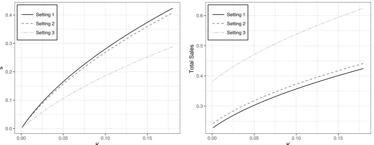
For each of these 4 cases, we compute the optimal uniform subsidys∗ and the optimal expected total
salesS∗ by varying the budgetK from 0 to 0.18. Our numerical results are summarized in Figures 5, 6,
7, and 8. In each figure, we depict the optimal subsidys∗ on the left panel and the total expected sales
S∗ on the right panel.
0.0 0.1 0.2 0.3 0.4
0.00 0.05 0.10 0.15
K
s
Setting 1 & 2 Setting 3
0.3 0.4 0.5 0.6
0.00 0.05 0.10 0.15
K
Total Sales
Setting 1 & 2 Setting 3
Figure 5 Optimal uniform subsidy (left) and the corresponding total sales (right) when the market sizeM is deter-ministic withm= 1.
We now observe:
1. The optimal per unit subsidys∗is the lowest in setting 3, followed by that in setting 2. This implies
that the donor can afford to reduce its per unit subsidy s∗ when there are more products available in
the market (as in Setting 2), and can reduce the subsidy even further when there is retail competition
(as in setting 3).
2. Combining observation 1 above with our analytical observation that the budget constraint is
bind-ing in all three settbind-ings, we see that the optimal total sales is the highest in Settbind-ing 3, followed by Settbind-ing