City, University of London Institutional Repository
Citation
:
Boon, M. Y., Henry, B. I., Chu, B. S., Basahi, N., Suttle, C. M., Luu, C., Leung, H. & Hing, S. (2016). Fractal Dimension Analysis of Transient Visual Evoked Potentials:Optimisation and Applications. PLoS One, 11(9), e0161565. doi: 10.1371/journal.pone.0161565
This is the published version of the paper.
This version of the publication may differ from the final published
version.
Permanent repository link: http://openaccess.city.ac.uk/16038/
Link to published version
:
http://dx.doi.org/10.1371/journal.pone.0161565Copyright and reuse:
City Research Online aims to make research
outputs of City, University of London available to a wider audience.
Copyright and Moral Rights remain with the author(s) and/or copyright
holders. URLs from City Research Online may be freely distributed and
linked to.
City Research Online: http://openaccess.city.ac.uk/ [email protected]
Fractal Dimension Analysis of Transient
Visual Evoked Potentials: Optimisation and
Applications
Mei Ying Boon1‡*, Bruce Ian Henry2‡, Byoung Sun Chu1¤a, Nour Basahi1, Catherine May Suttle1¤b, Chi Luu3,4, Harry Leung5¤c, Stephen Hing5
1School of Optometry and Vision Science, UNSW Australia, Sydney, New South Wales, Australia,2School of Mathematics and Statistics, UNSW Australia, Sydney, New South Wales, Australia,3Centre for Eye Research Australia, Royal Victorian Eye and Ear Hospital, East Melbourne, Victoria, Australia,4Department of Surgery (Ophthalmology), Melbourne Medical School, The University of Melbourne, Parkville, Victoria, Australia,5Park Road Eye, Hurstville, New South Wales, Australia
¤a Current address: School of Optometry and Vision Science, Catholic University of Daegu, Gyeongsangbuk-do, Republic of Korea
¤b Current address: School of Health Sciences, Optometry and Visual Sciences, City University, London, United Kingdom
¤c Current address: Southern Ophthalmology, Kogarah, New South Wales, Australia.
‡These authors are joint senior authors on this work.
Abstract
Purpose
The visual evoked potential (VEP) provides a time series signal response to an external visual stimulus at the location of the visual cortex. The major VEP signal components, peak latency and amplitude, may be affected by disease processes. Additionally, the VEP con-tains fine detailed and non-periodic structure, of presently unclear relevance to normal func-tion, which may be quantified using the fractal dimension. The purpose of this study is to provide a systematic investigation of the key parameters in the measurement of the fractal dimension of VEPs, to develop an optimal analysis protocol for application.
Methods
VEP time series were mathematically transformed using delay time,τ, and embedding dimension,m, parameters. The fractal dimension of the transformed data was obtained from a scaling analysis based on straight line fits to the numbers of pairs of points with sepa-ration less thanrversus log(r) in the transformed space. Optimalτ,m, and scaling analysis were obtained by comparing the consistency of results using different sampling frequen-cies. The optimised method was then piloted on samples of normal and abnormal VEPs.
Results
Consistent fractal dimension estimates were obtained usingτ= 4 ms, designating the fractal dimension =D2of the time series based on embedding dimensionm= 7 (for 3606 Hz and
a11111
OPEN ACCESS
Citation:Boon MY, Henry BI, Chu BS, Basahi N, Suttle CM, Luu C, et al. (2016) Fractal Dimension Analysis of Transient Visual Evoked Potentials: Optimisation and Applications. PLoS ONE 11(9): e0161565. doi:10.1371/journal.pone.0161565
Editor:Francisco J. Esteban, Universidad de Jaen, SPAIN
Received:December 7, 2015
Accepted:June 30, 2016
Published:September 6, 2016
Copyright:© 2016 Boon et al. This is an open access article distributed under the terms of the
Creative Commons Attribution License, which permits unrestricted use, distribution, and reproduction in any medium, provided the original author and source are credited.
Data Availability Statement:All the relevant data are contained within the paper.
Funding:This study was supported by a UNSW Australia Goldstar Award grant. The funders had no role in study design, data collection and analysis, decision to publish, or preparation of the manuscript.
5000 Hz),m= 6 (for 1803 Hz) andm= 5 (for 1000Hz), and estimatingD2for each embed-ding dimension as the steepest slope of the linear scaling region in the plot of log(C(r)) vs log(r) provided the scaling region occurred within the middle third of the plot. Piloting revealed that fractal dimensions were higher from the sampled abnormal than normal ach-romatic VEPs in adults (p = 0.02). Variances of fractal dimension were higher from the abnormal than normal chromatic VEPs in children (p = 0.01).
Conclusions
A useful analysis protocol to assess the fractal dimension of transformed VEPs has been developed.
Introduction
Visual evoked potentials (VEPs) are electrophysiological signals in response to temporally modulated stimuli recorded by electrodes located on scalp overlying the visual cortex. Such VEPs mainly reflect functional integrity of the visual pathway processing stimuli in the central visual field [1]. Visual evoked potentials may be used to indicate the health, normality and maturity of the visual system [1–3].
The International Society of Clinical Electrophysiology and Vision (ISCEV) has defined protocols for clinical assessment and the analysis of the VEP waveforms [1]. Transient VEPs record visual processing following a stimulus change. A typical VEP signal has a waveform appearance with peaks and troughs. The ISCEV protocol specifies the measurement of the amplitudes of the peaks and troughs and their latency, i.e., the time since the stimulus change. These measurements provide information about the speed and strength of processing arising from the cortical generators of the VEP components [1].
More generally, the VEPs contain fine detailed and possibly non-periodic structure. The importance of these aspects for normal visual processing is not yet clear. One method that has been used recently to provide an understanding of non-periodic structures in VEPs is the mea-surement of the fractal dimension of the time series [4–7]. Fractal dimensions may be used to quantify the complexity of a pattern by characterising how detail in the pattern changes with the scale in which it is measured. Fractal dimension measurements have been proven to be use-ful for quantifying chaotic, or non-linear deterministic, dynamical systems. Fractal structures may be identified in chaotic time series using Grassberger and Procaccia’s algorithm [8,9]. The fractal dimension provides an indication of the minimum number of first order differential equations, equivalent to the minimum number of dynamical variables required to model the behaviour of the dynamical system [8,9]. In previous studies the VEP has been found to behave as part of a nonlinear deterministic dynamical system characterized by fractal dimen-sions [4–7]. In the framework of nonlinear dynamical analysis, the VEP is regarded as a time series which images the electrophysiological activity of the visual system in the time domain for a fixed window of time. The VEP time series as specified in the ISCEV protocol is an ensemble average across multiple observations with the same stimulus. The averaging is neces-sary to remove EEG activity that is not related to the stimulus change.
in the electrophysiological activity of single neuronal populations [12]. It should be noted, however, that the transient VEP, recorded according to the ISCEV protocol is averaged to min-imise the input of noise. Consequently, the complexity of all brain dynamics are not being investigated, but a subset of dynamics restricted to the visual system [13]. The fractal dimen-sion measurement as applied in this study is not as a test for chaotic time series, but as a repro-ducible and reliable measurement for characterizing VEPs that is complementary to amplitude and latency measures.
Commercial VEP systems typically record transient VEPs using 1000 Hz sampling fre-quency. While sampling frequency does not impact greatly on the evaluation of amplitude and latency, the number of data points in the time series limits the accuracy of the estimate of the fractal dimension using Grassberger and Procaccia’s algorithm [14,15]. A higher number of data points and higher sampling frequencies allow higher fractal dimensions to be estimated with improved accuracy [14,15]. Abnormal visual systems might have higher dimensions than normal systems hence the use of sampling frequencies>1000 Hz might be useful. Higher sam-pling frequencies may also facilitate the examination of finer detail in the VEP through other measures such as detrended fluctuation analysis [16].
One potentially useful clinical application for the fractal dimension would be to assist in the differentiation of normal and abnormal visual systems. However, when computing the fractal dimension, there are a number of parameters and decision rules that must be optimised as the characteristics of the time series and the underlying dynamics of the system generating the time series on which these parameters depend are not knowna priori. If the fractal dimension is to find application in the analysis of clinical signals, a consistent set of protocols for its mea-surement must be devised. In previous work, the values of these parameters were optimised for the analysis of transient VEPs recorded with a 1000 Hz sampling frequency from children and adults with normal VEPs [5,6,17] but not for other sampling frequencies or for VEPs recorded from people with abnormal visual systems. This provides the primary motivation in this paper for the systematic investigation of the parameters in the measurement of the fractal dimension of VEPs in an effort to develop an optimal analysis protocol for clinical application. Our crite-ria for an optimal analysis protocol are that it yields fractal dimension estimates that are com-parable with previous work and producesD2estimates that are similar across different
sampling frequencies.
Materials and Methods
This study focuses on developing protocols for one fractal dimension measurement, the corre-lation dimension (D2) which is estimated using Grassberger and Procaccia’s algorithm [8,9],
for VEPs recorded using different commercially available sampling frequencies. This study was conducted in two phases. In the first phase, in recognition of the sequential nature of the esti-mation ofD2using the Grassberger and Procaccia algorithm, we developed the analysis
proto-col in stages such that later steps in the algorithm were only investigated after earlier steps were optimised. In the second phase, we applied the optimised protocol to a sample of VEPs recorded from adults and children, to investigate its ability to differentiate between VEPs drawn from normal and abnormal visual systems. As such, in both phases 1 and 2, the fractal dimension,D2, was the primary outcome variable that was analysed statistically. However, the
between stimulus onset and when the highest point in the peak, or lowest point in the trough. Components were repeatable if the peaks and troughs identified had latencies that were within 10% of the longest latency for two successive recordings of the VEP to the same visual stimulus [6].
In Phase 1, the key parameters investigated in the measurement ofD2are the delay timeτ
and the embedding dimensionm.D2is estimated from scaling behaviour at fixed values ofτ
andm. Custom software was written using Matlab (The Mathworks, Inc., Massachusetts, United States) to determine suitable values for these parameters. In Phase 2, the optimised method was then piloted on samples of normal and abnormal VEPs. The persons carrying out the analysis were unaware whether the VEPs they were analysing were drawn from normal or abnormal visual systems.
The study protocol, including the consent procedure, was approved by human research ethics committees (UNSW Australia Human Research Ethics Committee approval number: 09364 and SingHealth CIRB Secretariat Reference Approval Number: R1083/98/2013). All participants were provided with study participant information and consent forms and were given the opportunity to ask questions of the researchers to clarify any concerns. As the chil-dren had varying levels of reading and writing ability, the information in the consent form was conveyed to the children by the researchers either verbally or in written format. After agreeing to participate in the study, the participants>18 years of age gave their written con-sent and signed the concon-sent forms. In the case of child participants, the guardian/parent of each child gave their written consent and signed the consent forms after agreeing to allow their child to participate in the study. The child participants provided their assent, verbally, to the best of their ability to understand. The original signed copies of the informed consent forms are stored by the investigators in a secure location in accordance with the human research ethics committee documentation. The tenets of the Declaration of Helsinki were fol-lowed throughout.
Visual evoked potential sample characteristics
Samples of VEPs were drawn randomly from a dataset which included VEPs recorded from children and adults with normal and abnormal visual systems. Normal vision was defined as having normal visual acuity (6/6 Snellen visual acuity or better), no congenital colour vision deficiencies (Ishihara pseudoisochromatic colour vision screening test was used), normal stere-opsis (<50 seconds of arc) and no sign of ocular abnormality (evaluated using direct ophthal-moscopy). The abnormal VEPs were recorded in children and adults with known
abnormalities of visual pathway function including amblyopia, strabismus and central retinal artery occlusion [18]. The diagnosis of normality or otherwise was confirmed by ocular and visual system evaluation by registered optometrists and ophthalmologists.
Application and optimisation of parameters for dimension estimation
The application of Grassberger and Procaccia’s algorithm to transient VEPs has been described previously and is briefly reviewed here [5,6]. In this method, the VEP is regarded as a time series that is one observation of the dynamics of a deterministic system. For VEPs the deter-ministic system would be a mathematical model for the average electrophysiological processing of the visual system following a given stimulus change. If a system is deterministic, then any activity that occurs at one point in time must be dependent on activity that occurred earlier in the time series. The time evolution of the system that produces the VEP can be represented as a path, or phase space trajectory, in an abstract mathematical space called phase space. Using the time series for just one of the components (in this case the average observation that is the VEP) of the system, it is possible to reconstruct a path that shares the same invariant properties (such as dimension) as the full phase space trajectory. This process of reconstruction is called phase space embedding. If the reconstructed phase space hasmdimensions, then each reconstructed phase space coordinateXiis anmcomponent vector which is obtained from the time seriesy(t1),y(t2),. . .by the prescriptionXi= (y(ti),y(ti+τ),y(ti+2τ),. . .,y(ti+((m-1)τ) wheremandτ
are constant parameters, referred to as the embedding dimension, and the delay time, respec-tively. The indexidenotes ordering in time. Phase space trajectories of deterministic dynamical systems usually evolve towards a particular set of coordinates called an attractor, although this may be a transient attractor in the case of VEPs, and the dimension of the attractor is less than that of the full phase space. Grassberger and Procaccia’s algorithm can be used to characterise the phase space filling properties of the path. The dimension is obtained by covering the set with boxes of a given size (r) and then computing the probabilitypi(r) (equivalent to the
rela-tive frequency in sufficiently large data sets) of having a point of the set in theith box. The cor-relation dimension (D2) for a set of points is formally defined as:
D2¼rlim!1
logXip2iðrÞ
logr ðEq 1Þ
wherep2iðrÞis the probability offinding a pair of points in a box of sizer. The limitrto zero is not amenable to real world data and instead some scaling relations are used. Grassberger and Procaccia [8,9] found that for small values ofrand for sufficiently large numbers of data points,N, the probability of having a pair of points in a box of sizeris the same as the probabil-ity of having a pair of points with separation distance less thanr. This latter probability is the correlation sum described by the following formula:
CðrÞ ¼ lim
N!1
1
ðNðN1Þ
:number of pairs of points with separation<r ðEq 2Þ
For smallr, the correlation sum grows according to a scaling relationCðrÞ rD2. This scal-ing relation is only valid ifris small andNis large and this needs to be borne in mind in appli-cations. Rearranging the scaling relation and taking logarithms of both sides, shows thatD2
may be approximated by log (C(r))/log(r), which is usually approximated as the slope of the straight line scaling region in a plot of log(C(r)) vs log(r).
When used to estimate the correlation dimension of a time series, the time series is embed-ded into a range of phase space dimensions,m. The dimensionD2is estimated for each
It can be seen that a number of key decisions must be made. As sampling frequency is var-ied, what are appropriate values for the delay timeτ? From which range of embedding dimen-sions should the fractal dimension,D2,be measured? How should the straight line scaling
region be identified in the plot of log(C(r)) vs log(r)? These questions are considered below.
Considerations in the selection of delay time,τ. Ifτis too small, theny(ti+τ) is almost
the same asy(ti) and therefore a reconstructed attractor will lie nearly on a straight line with
D2= 1. Ifτis too large, the time series points may be too widely separated in time to be
consid-ered as components of a single phase space vector. In this case there may be no discernible struc-ture in the reconstructed phase space trajectory [20]. Thereforeτshould be selected so that the reconstructed trajectory is not stretched out along the diagonal in the embedding space [21,22]. For embedding dimensions less than four this can be seen in a simple visual plot of the trajectory [5]. In previous studies, for VEP data recorded at 1000 Hz sampling frequency,τof 4 or 6, equiv-alent to 4 or 6 ms in the time domain, permitted the fractal dimension of VEPs in children and adults to be estimated and distinguished from each other [5,6,17]. In this study delay times of τ= 1, 3, 6, 9, 13, 16, 19, 22 and so on were trialled on VEPs recorded at sampling frequencies
>1000 Hz. Our guiding principle was to select the smallest values forτthat revealed structures other than thin lines stretched out along the diagonal in the reconstructed phase space trajecto-ries with very little change in structure for a range of increasingτ[21].
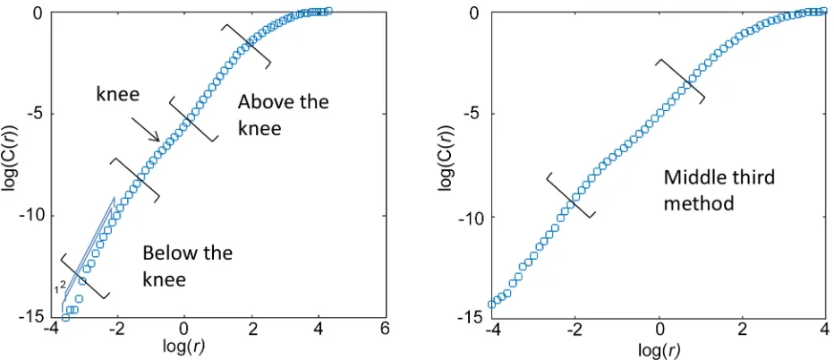
[image:7.612.111.577.463.664.2]Considerations regarding the scaling analysis. The scaling region within the plot of log (C(r)) vs log(r) does not always cover the entire plot. Recall that the scaling relation was depen-dent onrbeing small andNbeing large however there is a minimumr, below which no pairs of points would be in a box, and there is a maximumr, above which all pairs of points would be in the box. Slopes should be calculated from a range of box sizes,r, between these extremes. Henry et al. [21] suggested using the middle third of the data to estimate slope (seeFig 1). The criterion of the middle third rule objectively avoids the smallest scales for which fluctuations are great and the largest scales that are constrained by the finite number of data points in a dis-crete time series. This is an objective measure but it may cross changes in slope, such as for those plots of log(C(r)) vs log(r) which contain a“knee”, where the plot appears to bend in a
Fig 1. Two methods of finding the scaling region in sample plots of log(C(r)) vs log(r) are illustrated: Above and below the knee, and the Middle Third Rule.The numbers in blue,“1, 2”, indicate two consecutive running average slopes of 12 consecutive data points.
manner similar to a knee. Tsonis et al. [23] showed in a plot of slope as a function of log(r) that very small scales tend to show large fluctuations in slope. Tsonis et al. [23] does not suggest using the middle third to estimateD2but agreed thatD2should be estimated from an
interme-diate region, and suggested using the widest plateau in the plot of slope as a function of log(r) as it would be the most stable scaling region. Note that this will not typically occur for the smallest and largest values ofr.
Some researchers have suggested measuring the slope above, below, or at a tangent along the knee [24]. The importance of the presence or absence of a“knee”in relation to VEP data is not known and is worth further investigation. One possible explanation for a knee is that the data is noise on scalesbelowthe knee but is deterministic on scales above the knee. In this case we would expect to measureD2=mbelow the knee since noise is space filling, or approaching
min the case of data- limited noise, andD2<mabove the knee as deterministic structure is
expected to be non-space filling.
To estimateD2for each embedding dimension,m, we first computed a running average
slope over 12 consecutive data points in the plot of log(C(r)) and log(r), and then made plots of the running average slope as a function of log(r). Three strategies were then considered: (i) If a knee was present in this plot, slope was estimated above the knee and below the knee separately
(seeFig 1) providing two values forD2for a givenmbased on the corresponding plateau values.
(ii)D2for a givenmwas estimated as the largest value within the widest plateau region. (iii) If
the widest plateau in the plot of running average slope as a function of log(r) occurred within the middle third,D2for a givenmwas estimated as the largest value from the plateau within
the middle third.
To determine if the values ofD2obtained for each embedding dimension were indicative of
either deterministic structure or noise, we plottedD2as a function of the embedding dimension
m. The characteristic feature of deterministic structure in this plot is thatD2limits to a ceiling
value less thanm. This shows up as a plateau in the plot ofD2versusm. To determine whether
D2reached a ceiling value in this plot we measured a plateau index PI [5] defined as:
PI¼D2ðmÞ D2ðm1Þ ðEq 3Þ
wheremis the maximummallowed by the data according to the Eckmann-Ruelle criteria [14],
m ð2log10ðNÞÞ ðEq 4Þ
whereNis the number of data points We took PI<0.3 as the indicator thatD2had reached a
ceiling value [5].
Our criterion for an optimal scaling method is that it results in an unambiguous measure of slope for all VEPs and yields estimates ofD2that are comparable with previous work [5,6]
Comparability of fractal dimension estimates for different sampling frequencies, embedding dimension considerations. To check whether the parameters and rules yielded by the above strategies are unaffected by sampling frequency, it is necessary to compareD2for
VEPs identical in every way except for the sampling frequency using the optimised method. A higher sampling frequency provides more data points,N, and hence a greater maximum embedding dimension,m, (seeEq 4), and a greater possible correlation dimension,D2m.
The fractal dimensionD2was computed for VEP time series at their originally recorded
m= 7 for 3606 and 5000 Hz sampling frequencies,m= 6 for 1803 and 2500 Hz sampling
fre-quencies andm= 5 for 1000 Hz sampling frequencies for our calculations.
Statistical analysis
This study was carried out in two phases and the primary outcome measure of interest wasD2
for each of the phases. The purpose of the first phase was to determine the protocol; family-wise Type 1 error was controlled by using a Bonferroni-Sidak correction to adjust theαby the total number of statistical analyses conducted, 3, to 0.017. In the second phase, in which the protocol was piloted on samples of VEPs drawn from normal and abnormal visual systems, an Analysis of Variance test with Bonferroni corrections of the post-hoc paired comparisons were conducted, to control family-wise Type 1 error.
Results
Phase 1: Optimising the analysis protocol
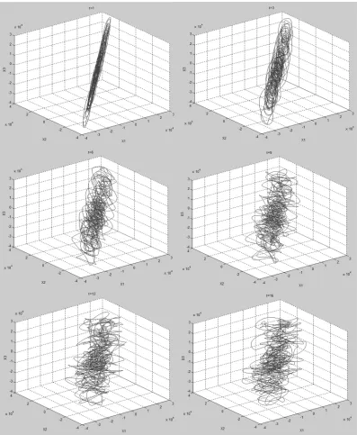
Delay time,τ. Fig 2shows typical plots of the reconstructed phase space trajectories for differentτvalues. The plots shown are from a VEP of a child with abnormal vision due to amblyopia (initials LS) recorded using a 3606 Hz sampling frequency in response to black and white sine wave gratings. Forτ16 data points (4.4 ms), the shape of the reconstructed trajec-tory appears to be topologically stable (i.e. has geometric properties preserved despite deforma-tions such as stretching) under rotation when viewed in Matlab, and not simply stretched along the diagonal.Fig 2andTable 1show that while delay time in terms of number of data points changes with sampling frequency, the shortest useful delay time for VEPs recorded at 3606 and 5000 Hz sampling frequency is about 4 ms.
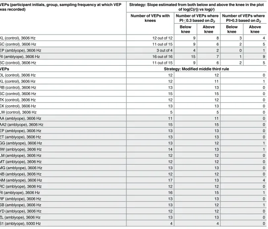
The scaling analysis. In the log-log plots of C(r) versusr, a knee was present in 42 out of 47 cases. Two slopes were estimated, one below the knee and the other above the knee. The proportion of slopes with PI<0.3 (seeEq 3) was significantly less for those estimated from “above the knee”than“below the knee”(Chi square with Yates correction = 8.57, p = 0.003). These slopes were visualised as the two widest plateaus within the plot of running average slope vs log(r). The strategy of finding the scaling region above the knee and below the knee did not work well as a large proportion of the VEPs did not result in PI0.3 (Table 2). Further, the magnitude ofD2was evaluated for a subset of VEPs analysed usingτ= 16,k= 12 and
excluding those VEPs which resulted in missing data (i.e. PI>0.3 for one or both below or above kneeD2estimates). Mean (SD) estimates ofD2from below the knee, and above the knee,
were 4.02 (0.83) and 2.70 (0.35), respectively and were significantly different (F1, 12= 25.15,
p<0.0001). These findings are consistent with a previous study [25] on electrocardiograms that found theD2estimate below the knee is usually higher than theD2estimate from above
the knee, although the significance of both was uncertain.
It was not possible to reliably estimateD2from the largest value in the widest plateau region
in the plot of running average slope vs log(r) because it was difficult to define the extent of the plateau, particularly its start and end points. Sometimes, more than one plateau in a plot had the same width. Due to these ambiguities, the analysis could not continue to aD2estimate.
When an additional criterion was added that the widest plateau fell within the middle third of the plot [21], this resulted in reliable and unambiguous estimates with PI<0.3 (Table 2). This method is a modification of the Middle Third Rule [21].
Estimates ofD2at original and halved sampling frequency were highly correlated R = 0.99 (Fig
3). There were no significant differences in the estimates ofD2(F1, 9= 0.00, p = 0.99, mean
dif-ference = 0.00). These results were found by estimating fractal dimension fromD2at m = 7 for
[image:10.612.179.576.76.559.2]VEPs sampled at 3606 and 5000 Hz,m= 6 for 1803 Hz andm= 5 for 1000 Hz. Fig 2. Reconstructed phase space trajectories of a VEP recorded with 3606 Hz sampling frequency embedded in 3 dimensional phase space using different values ofτ.From top left to bottom right,τ= 1, 3, 6, 9, 13, 16, 19, 22.
Phase 2: Piloting the optimised method
The VEPs analysed were from a group of adults with normal (n = 4) and abnormal (n = 8) visual systems, recorded using the Medelec Synergy system with a 1000 Hz sampling frequency, single band pass filtered (1–50 Hz), with the 50 Hz notch filter applied to exclude mains elec-tricity noise. The abnormal visual systems in the adults were due to a variety of causes includ-ing amblyopia, strabismus, pathological myopia and retinal vein occlusion. Visual evoked potentials in response to black-white (100% luminance contrast) and isoluminant magenta-cyan (42% chromatic contrast) gratings were analysed and compared between the normal and abnormal visual systems. Grassberger and Procaccia’s algorithm was implemented usingτas the closest approximation for 4.4 ms. The Shapiro-Wilk test [26] indicated the data were nor-mally distributed. Analysis of variance was run with stimulus type (black-white or red-green) and viewing condition (monocular or binocular) as within subjects factors, group (normal or abnormal) as the between group factor and adjustment for multiple comparisons (Bonferroni correction). Estimated marginal means forD2were 2.79 (95%CI 2.62–2.95) for the control
group and 3.08 (95% CI 2.91–3.25) for the abnormal group and were found to be statistically significantly different (p = 0.02).
For descriptive purposes,Fig 4presents the group average binocular VEPs in response to black-white 2 cpd sinusoidal gratings for the two adult groups. The standard ISCEV nent CI, CII and CIII amplitudes and latencies were determined. Mean (SD) of VEP compo-nents are presented inTable 3.
[image:11.612.35.583.97.296.2]Data comprising binocular VEPs in response to magenta-cyan isoluminant gratings recorded from a group of children with normal (n = 5) and abnormal visual systems (n = 13), with a 3606 Hz sampling frequency using a Diagnosys electrophysiology system, and no band pass filter or notch filter to exclude mains noise, were analysed. Grassberger and Procaccia’s algorithm was implemented usingτ= 16, which corresponded to a delay time of 4.4 ms. All the children with abnormal visual systems had amblyopia associated with either strabismus or refractive error and were undergoing treatment. Although the Shapiro-Wilk test [26] indicated the data were normally distributed, Levene’s test [27] indicated that the variances were
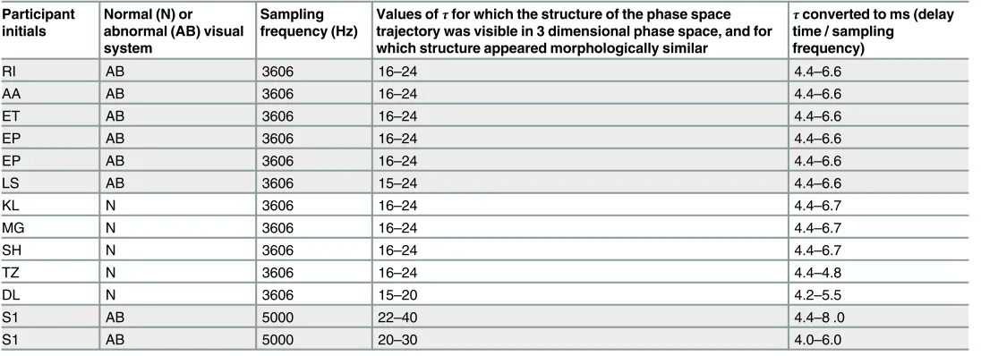
Table 1. Range of values forτfor VEPs recorded at>1000 Hz such that reconstructed phase space trajectories were not stretched along the diago-nal such that fluctuations in the trajectory were evident.
Participant initials
Normal (N) or abnormal (AB) visual system
Sampling frequency (Hz)
Values ofτfor which the structure of the phase space trajectory was visible in 3 dimensional phase space, and for which structure appeared morphologically similar
τconverted to ms (delay time / sampling frequency)
RI AB 3606 16–24 4.4–6.6
AA AB 3606 16–24 4.4–6.6
ET AB 3606 16–24 4.4–6.6
EP AB 3606 16–24 4.4–6.6
EP AB 3606 16–24 4.4–6.6
LS AB 3606 15–24 4.4–6.6
KL N 3606 16–24 4.4–6.7
MG N 3606 16–24 4.4–6.7
SH N 3606 16–24 4.4–6.7
TZ N 3606 16–24 4.4–4.8
DL N 3606 15–20 4.2–5.5
S1 AB 5000 22–40 4.4–8 .0
S1 AB 5000 20–30 4.0–6.0
Shaded cells indicate abnormal VEPs.
significantly different (Levene statstic1,15= 7.76, p = 0.01), as illustrated in the boxplots inFig 5. Hence the non-parametric independent samples median test was used to investigate between group differences, for which no significant difference in the medians was found (p = 1.0).Fig 5 shows that the abnormal group had more extreme tails than the normal group forD2.Fig 6
shows the children’s VEPs, including those that had the extremely high or lowD2. CI and CII
were not consistently repeatable. Therefore only the CIII component latencies could be reliably estimated for all children, as CIII amplitude depended on the CII component being repeatable
[image:12.612.38.579.86.549.2](Table 3).
Table 2. Comparison of strategies for finding the scaling region.
VEPs (participant initials, group, sampling frequency at which VEP was recorded)
Strategy: Slope estimated from both below and above the knee in the plot of log(C(r)) vs log(r)
Number of VEPs with knees
Number of VEPs where PI0.3 based onD2
Number of VEPs where PI>0.3 based onD2
Below knee Above knee Below knee Above knee
KL (control), 3606 Hz 12 out of 12 9 8 3 4
SC (control), 3606 Hz 11 out of 15 9 6 2 5
EP (amblyope), 3606 Hz 3 out of 4 4 2 0 1
RI (amblyope), 3606 Hz 16 out of 16 15 7 1 9
SC (control), 3606 Hz 11 out of 15 9 6 2 5
VEPs Strategy: Modified middle third rule
DL (control), 3606 Hz 12 12 0
KL (control), 3606 Hz 12 11 1
RB (control), 3606 Hz 13 13 0
SC (control), 3606 Hz 15 15 0
TK (control), 3606 Hz 12 12 0
EK (control), 3606 Hz 13 13 0
LW (control), 3606 Hz 5 5 0
AA (amblyope), 3606 Hz 11 11 0
AA2 (amblyope), 3606 Hz 15 15 0
EP (amblyope), 3606 Hz 13 13 0
ET (amblyope), 3606 Hz 13 13 0
GG (amblyope), 3606 Hz 13 12 1
JW (amblyope), 3606 Hz 14 13 1
LM (amblyope), 3606 Hz 12 12 0
MT (amblyope), 3606 Hz 12 12 0
MG (amblyope), 3606 Hz 13 13 0
NB (amblyope), 3606 Hz 12 12 0
NM (amblyope), 3606 Hz 17 13 4
RC (amblyope), 3606 Hz 12 12 0
RI (amblyope), 3606 Hz 16 15 1
RF (amblyope), 3606 Hz 13 13 0
SB (amblyope), 3606 Hz 13 12 1
YD (amblyope), 3606 Hz 12 12 0
ZL (amblyope), 3606 Hz 13 13 0
S1 (amblyope), 5000 Hz 4 4 0
PI = Plateau Index. Shaded cells indicate abnormal VEPs.
Discussion
A central part of this study was to determine if useful protocols could be established for mea-suringD2from VEPs of different sampling frequencies. The results confirmed a useful protocol
could be established for all VEPs recorded at 1000, 3606 and 5000 Hz sampling frequencies. The results suggest that useful estimates ofD2may be obtained using the protocol described in
this study.
The significance of the presence or absence of a“knee”remains unclear as knees were not always present and it was not always possible to obtain a reliable estimate ofD2using the slope
above and below the knee. This suggests that trying to estimateD2with reference to a knee is
an unreliable method of estimatingD2. The presence of two scaling regions separated by a
knee, if they occurred, might reflect different physiological processes. In cases where they could be reliably measured, the mean difference between the slopes of the scaling regions below and above the knee was relatively large at 1.32, given that 0.5 is the difference between mature and immature visual systems, [6]. The scaling below the knee was not equivalent tomhowever it approachedm, which may be consistent with an interpretation of data-limited space filling noise, for most of the VEPs. The scaling below the knee was more likely to demonstrate PI<0.3 (seeEq 3) than above the knee (seeTable 2). The above suggests that trying to estimateD2with
reference to a knee is an unreliable method of estimatingD2. Other possible explanations for
[image:13.612.200.456.74.316.2]the presence of a“knee”are either excessively high levels of correlation among nearby data points in the time series or use of an excessively largeτsuch that there is loss of correlation between components of points in phase space [24]. Excessively high or low levels of correlation for a givenτmight indicate an unusual physiology. However, as VEPs from both amblyopic and normal visual systems were found to have knees while using a delay time of 4.4 ms, which appears to be appropriate using other criteria, it does not appear to reflect abnormality of phys-iology. Slope estimation from the widest plateau in the middle third is an alternative method which does not depend on the presence of a“knee”.
Fig 3. Scatterplot ofD2estimated from VEPs from full and halved sampling frequencies for the same
delay times of 4.4 ms.
Within the limitations outlined, VEPs recorded from different electrophysiology systems using different sampling frequencies may yield comparable estimates ofD2provided the data
[image:14.612.160.575.72.383.2]are analysed within the parameters as outlined in this paper. However it must be noted that comparison of VEPs recorded from multiple set-ups or sites still requires care as it is likely that differences between laboratories extend to more than just the selection of sampling frequency. Fig 4. Adult binocular VEP responses to black and white pattern onset-offset grating stimuli.(a) Abnormal and (b) Normal adult binocular VEP responses. The components CI, CII and CIII and stimulus onset and offset times are shown for illustration purposes in (a). The group averaged responses are in bold. Individual responses, which were the average of two recordings, are presented as the thinner lines.
doi:10.1371/journal.pone.0161565.g004
Table 3. Group mean (SD) of VEP component amplitude and latency data.
Group Stimulus CI amplitude
(μV)
CI latency (ms)
CII amplitude (μV)
CII latency (ms)
CIII amplitude (μV)
CIII latency (ms)
Adult Control Black-white gratings
0.28 (1.77) 87.75 (14.52) -1.42 (1.08) 117.00 (12.08)
2.67 (1.14) 193.50 (21.56)
Adult (Abnormal visual system)
Black-white gratings
1.38 (1.93) 76.00 (6.16) -6.10 (3.14) 123.00 (10.07)
11.56 (5.82) 193.50 (19.76)
Child Control Magenta-cyan gratings
1.77 (5.88) 63.52 (14.88) -10.11 (8.62) 88.44 (25.74) 35.5 (8.23) 147.4 (6.9)
Child (Abnormal visual system)
Magenta-cyan gratings
175.38 (20.1)
The cells in grey indicate abnormal visual system data. Where components were not repeatable in latency for a group, mean (SD) are not reported for that group and the cells are shaded dark grey.
[image:14.612.35.580.551.667.2]For example, differences in the kinds of equipment used such as electrode type, levels of electri-cal noise in the immediate surrounds and characteristics of the stimulus display may also impact on the morphology of the VEP recorded. In recognition of this fact, ISCEV acknowl-edges that VEP waveforms are expected to be similar across laboratories when recorded under standard conditions but when seeking to differentiate between normal and abnormal, each lab-oratory should establish its own set of normative values [1].
The protocols developed here appear to yield estimates ofD2for visual processing of stimuli
that are comparable to estimates found in previous research [6]; ranging between 2 and 3.25 for binocular VEPs in response to magenta-cyan stimuli in children and adults. Taking the number of independent components composing a signal as the nearest integer aboveD2, this
suggests that there may be somewhere between two and four independent components in these VEPs. This result also agrees with other analyses which measure the number of underlying components using different methods. For example, Maier et al. [12] used principal components analysis (PCA) on recordings between multiple scalp electrode sites to estimate the number of dipole sources that are active in the visual electrophysiological response to visual stimulation. They found that only two components are necessary to explain 95% of the power of the responses of the 24 electrodes they used for any stimulus type, and attributed the remaining 5% to noise. Almurshedi and Ismail [28] also determined that although PCA may yield five princi-pal components (PCs), only the first two appeared to be strongly related to the signal. Zhang and Hood [29] found three significant principal components. They determined that, of these, the first (PC1) was likely to be a component derived purely from V1 of the brain, and that PC2 may be attributed to a small area of the visual cortex or derived from the extrastriate cortex, or a combination of the striate and extrastriate cortex.
Two kinds of stimuli were used which evaluated different aspects of the visual system. The black and white stimuli preferentially stimulated the magnocellular pathways whereas the magenta-cyan stimuli preferentially stimulated the parvocellular pathways of the visual system. In our sample of adults’VEPs,D2was found to be higher overall in the abnormal, than the
nor-mal visual systems. In contrast, the children with abnornor-mal visual systems had VEPs in Fig 5.D2estimated using a delay time of 4.4 ms of VEPs in response to binocular magenta-cyan
stimulation in children with normal and abnormal visual systems.
[image:15.612.201.507.77.290.2]response to magenta-cyan stimuli which tended towards both higher and lower values ofD2
than normal, but did not differ on average. For behavioural measures, values which tend towards extremes may be indicative of abnormal populations even though average responses are similar to normal populations e.g. to reflect the overactivity or underactivity or a system [30,31].
Divergence between the adult and child findings might also be due to differences in the depth, type and severity of the visual system abnormality between the adults and the children. Adult participants exhibited long standing visual pathologies which ranged from ocular (e.g. vein occlusion) to cortical (e.g. amblyopia) and were resistant to different treatments. In con-trast, the children in our study had only one type of abnormality (amblyopia) and were already undergoing treatment so the severity and depth of the abnormality was related to their compli-ance and response to ongoing treatment.
There is evidence that adaptations within the visual system in response to altered sensory inputs may take considerable time to reach a measureable effect. For example, Codina et al. [32] found cross-modal plasticity in individuals with longstanding deafness; they had high visual function associated with the recruitment of parts of the auditory cortex for visual pro-cessing. As dynamical variables may relate to the number of neuronal populations, the recruit-ment of additional neuronal populations towards processing would be evident as increasedD2
[10,11]. Interestingly, Codina et al. [32] found that cross-modal plasticity was only observed in adolescents from 13 years of age and adults, but not in children. Our data are consistent with Codina et al.’s [32] findings as group average differences inD2are evident in the adult, but not
the child, data.
The magnitude ofD2may be reflected in ISCEV morphology, however our results can only
be suggestive rather than conclusive due to the small numbers in the high and lowD2groups in
both the adult and child samples. ViewingFig 6andTable 3, it appears that for the children with abnormal systems and higherD2, CIII amplitude appeared low compared to the children
with normal visual systems, and CI and CII were not consistently repeatable. In the children with abnormal visual systems and lowerD2, the main difference from normal seemed to be the
lack of a repeatable CI and CII. The CII component of the magenta-cyan VEP is typically less prominent in the immature visual system [33–35] hence their lack of repeatability in some of the abnormal VEPs might indicate changes in the development of the parvocellular pathways in those children. Studies suggest that CII may be more strongly related to the colour process-ing of the parvocellular system, whereas CIII is more related to the non-colour processprocess-ing func-tions [34,36]. The lack of repeatability in CI and CII components may indicate abnormalities in these aspects of cortical processing. The relationship betweenD2and the magnitude of
ISCEV VEP components requires further investigation.
This study has some limitations. As was discussed earlier, the ISCEV protocol for recording VEPs requires averaging to remove noise. Therefore some dynamics of brain processing are excluded by design. Overall brain function may impact on cortical processing of the visual sig-nal, for example through attentional or feedback processes which may be reflected in EEG Fig 6. Children’s VEPs in response to magenta-cyan pattern-onset offset grating stimuli analysed using the optimised protocol.(a) shows the children’s VEPs drawn from children with normal visual systems. (b) shows the abnormal VEPs, with the average of the three lowestD2VEPs in bold blue, the average of the three highestD2VEPs in bold red, and the remainder
of VEPs in bold black. Individual VEPs, which were the average of two recordings, are presented in grey. To illustrate the morphology of abnormal VEPs which tended towards the extremes of low and highD2more clearly, the three abnormal VEPs
with the lowest and highestD2are shown in (c) and (d) respectively. The group averaged responses are in bold. Individual
responses, which were the average of two recordings, are presented as the thinner lines.
microstates [37]. Future research could look further into those aspects, however the present study has made a start by evaluating the averaged VEP.
While normal and abnormal VEP data was included to pilot the optimised protocol, it was stated in the introduction that a potential application would be to characterise normal and abnormal VEPs and ideally,D2might even serve as an objective indicator of abnormality.
Although the optimised protocol yielded unambiguous measures ofD2that were comparable
to previous measures ofD2of the VEP and consistent with PCA estimates of numbers of
com-ponents involved, indicating that the optimised protocol functioned as desired, there was a lack of clearly significant average differences between normal and abnormal VEPD2measures in
the children’s sample. This may be for a number of reasons. As discussed earlier, they might have already been recovering function. Additionally, the visual stimuli used in the present study preferentially stimulated chromatic parvocellular visual pathways that may have been relatively unaffected by the condition for the sample. Perhaps the use of different stimuli that evaluate other types of cortical processing such as achromatic parvocelullar function[38], might yield larger differences in processing which might then be reflected by greater differences inD2. As Sloper[39] noted, although amblyopia can be manifest as losses in parvocellular and
magnocellular function, it is not a single uniform condition so the patterns of abnormalities will vary according to the types of abnormal visual experiences and the time periods in which they were experienced.
Summary of Key Findings
To estimate the fractal dimension of transient visual evoked potentials for averaged recordings of one second duration and 2 Hz temporal frequency, the following optimised analysis protocol should be used when applying Grassberger and Procaccia’s algorithm:
1. Use a delay time,τ, which corresponds to 4 ms.
2. Use 64 bins of box sizes,r.
3. The embedding dimensions,m, for whichD2should be estimated for each VEP, includes 1,
2, 3. . .mwheremis limited by the number of data points according to Eckman and Ruelle’s criterion (2log10(N)) [14]. Therefore,m= 7 for 3606 and 5000 Hz sampling
fre-quencies,m= 6 for 1803 and 2500 Hz sampling frequencies andm= 5 for 1000 Hz sam-pling frequency.
4. The scaling analysis strategy should be based on Henry et al.’s [21] and Tsonis’[23] criteria and not consider the knee. For eachm, running average slopes of 12 consecutive data points along the plot of log(C(r)) vs log(r) should be used to generate a plot of running average slope vs log(r) (Note log(r)is selected for its ordering value indicating the starting point on the plot of log(C(r)) vs log(r) from which the running average slope was calculated, rather than for its numerical value. InFig 7, the running average slopes are plotted as functions of their ordered calculation). The widest plateau in that plot should be identified. If the widest plateau falls within the middle third of the plot (indicated as the red crosses inFig 7), then the highest value for slope in the plateau within the middle third is the estimate ofD2for thatm.
5. Next, plotD2as a function ofm(see bottom right panel inFig 7). IfD2plateaus as it
approachesm, using the criterion that PI<0.3 [5], thenD2atmmay be used as an
esti-mate of the fractal dimension of the underlying system which produced that VEP.
6. Piloting the optimised method indicatedD2has the potential to increase understanding of
Conclusions
In conclusion, VEPs recorded from different electrophysiological recording systems using dif-ferent sampling frequencies may yield comparable estimates ofD2provided the data is
ana-lysed within the protocols outlined in this paper. This will assist in the comparison ofD2
measures between electrophysiology systems which employ different sampling frequencies, which enhances its applicability as a complementary objective measure of visual system electrophysiological activity as imaged using the VEP. Interpreting the nearest integer above
D2as the minimum number of independent components comprising the signal, is broadly
con-sistent with the results of principal component analysis. The development of a robust protocol for measuringD2,as undertaken here is an important step towards usingD2measurements
clinically.
Acknowledgments
We thank the participants and their families for volunteering. We thank Tiong Peng Yap for providing transient VEPs recorded at 5000 Hz sampling frequency for analysis. This study was supported by a UNSW Australia Goldstar Award grant.
Author Contributions
Conceived and designed the experiments:MB BH.
Performed the experiments:MB BH BC NB CS CL HL SH.
Analyzed the data:MB BH BC NB HL.
Contributed reagents/materials/analysis tools:MB BH HL SH.
Wrote the paper:MB BH BC NB CS CL HL SH.
Contributed to the experimental design of the mathematical analysis protocol: MB BH BC NB. Contributed to the design of the electrophysiology recording protocol: MB CS CL.
References
1. Odom JV, Bach M, Brigell M, Holder GE, McCulloch DL, Tormene AP, et al. ISCEV standard for clinical visual evoked potentials (2009 update). Documenta ophthalmologica Advances in ophthalmology. 2010; 120(1):111–9. Epub 2009/10/15. doi:10.1007/s10633-009-9195-4PMID:19826847.
2. McCulloch DL, Skarf B. Pattern reversal visual evoked potentials following early treatment of unilateral, congenital cataract. Archives of ophthalmology. 1994; 112(4):510–8. Epub 1994/04/01. PMID:
8155050.
3. Oner A, Coskun M, Evereklioglu C, Dogan H. Pattern VEP is a useful technique in monitoring the effec-tiveness of occlusion therapy in amblyopic eyes under occlusion therapy. Documenta ophthalmologica Advances in ophthalmology. 2004; 109(3):223–7. Epub 2005/06/17. PMID:15957607.
4. Arle JE, Simon RH. An Application of Fractal Dimension to the Detection of Transients in the Electroen-cephalogram. Electroen Clin Neuro. 1990; 75(4):296–305. PMID:ISI:A1990CY99000004.
5. Boon MY, Henry BI, Suttle CM, Dain SJ. The correlation dimension: a useful objective measure of the transient visual evoked potential? J Vis. 2008; 8(1):6 1–21. Epub 2008/03/06. doi:10.1167/8.1.6PMID:
18318609.
Fig 7. Depiction of the optimised analysis method.Top panel, example VEP. Intermediate panels show plots of log(C(r)) vs log(r) and plots of running average slope of log(C(r)) vs log(r) as a function of their ordered calculation for m = 1 to 7. The red crosses indicate the data derived from the middle third of the plot log(C(r)) vs log(r). The final panel is a plot ofD2for m = 1 to 7: the ceiling value at m = 7 is an indicator of the fractal
dimension of the system.
6. Boon MY, Suttle CM, Henry BI, Dain SJ. Dynamics of chromatic visual system processing differ in com-plexity between children and adults. J Vis. 2009; 9(6):22 1–17. Epub 2009/09/19. doi:10.1167/9.6.22
PMID:19761313.
7. Schmeisser ET, Hooper RW, Mcguiness M. Discrete Flicker Detection Perimetry in Glaucoma. Invest Ophth Vis Sci. 1993; 34(4):1265–. PMID:ISI:A1993KT89302769.
8. Grassberger P, Procaccia I. Measuring the Strangeness of Strange Attractors. Physica D. 1983; 9(1– 2):189–208. PMID:ISI:A1983RU46800010.
9. Grassberger P, Procaccia I. Characterization of Strange Attractors. Phys Rev Lett. 1983; 50(5):346–9. PMID:ISI:A1983PZ53000017.
10. Muller V, Lutzenberger W, Preissl H, Pulvermuller F, Birbaumer N. Complexity of visual stimuli and non-linear EEG dynamics in humans. Brain research Cognitive brain research. 2003; 16(1):104–10. Epub 2003/02/19. PMID:12589895.
11. Muller V, Lutzenberger W, Pulvermuller F, Mohr B, Birbaumer N. Investigation of brain dynamics in Par-kinson's disease by methods derived from nonlinear dynamics. Experimental brain research Experi-mentelle Hirnforschung Experimentation cerebrale. 2001; 137(1):103–10. Epub 2001/04/20. PMID:
11310163.
12. Maier J, Dagnelie G, Spekreijse H, van Dijk BW. Principal components analysis for source localization of VEPs in man. Vision research. 1987; 27(2):165–77. PMID:3576977.
13. Janosi IM, Tel T. Time-series analysis of transient chaos. Physical Review E. 1994; 49(4):2756–63.
14. Eckmann JP, Ruelle D. Fundamental limitations for estimating dimensions and Lyapunov exponents in dynamical systems. Physica D, Nonlinear Phenomena. 1992; 56:185–7.
15. Tsonis AA. Chaos: from theory to applications. New York: Plenum Press; 1992.
16. Peng CK, Buldyrev SV, Havlin S, Simons M, Stanley HE, Goldberger AL. Mosaic Organization of DNA Nucleotides. Physical Review E. 1994; 49(2):1685–9. doi:10.1103/PhysRevE.49.1685PMID:WOS: A1994NA92100094.
17. Boon MY, Suttle CM, Henry BI, Chu BS, editors. The fractal dimension as a potential indicator of recov-ery from amblyopia. The 13th Biennial Scientific Meeting, 7th Educators' Meeting in Optometry; 2011 2011; Sydney, Australia: Clinical and Experimental Optometry.
18. Kanski JJ. Clinical Ophthalmology, a systematic approach. Second ed. Hong Kong: Butterworth-Hei-neman Lit; 1989.
19. Odom JV, Bach M, Barber C, Brigell M, Marmor MF, Tormene AP, et al. Visual evoked potentials stan-dard (2004). Documenta ophthalmologica Advances in ophthalmology. 2004; 108(2):115–23. PMID:
15455794.
20. Mizrach B. Determining delay times for phase space reconstruction with application to the FF/DM exchange rate. Journal of Economic Behavior & Organization. 1996; 30:369–81.
21. Henry B, Lovell N, Camacho F. Chapter 1. Nonlinear dynamics time series analysis. In: Akay M, editor. Nonlinear biomedical signal processing volume II, dynamic analysis and modelling, II. II. New York: IEEE Press Series on Biomedical Engineering; 2001. p. 1–39.
22. Kostelich EJ, Swinney HL. Practical considerations in estimating dimension from time series data. Phy-sica Scripta. 1989; 40:434–41.
23. Tsonis AA. Dynamical changes in the ENSO system in the last 11,000 years. Clim Dynam. 2009; 33(7– 8):1069–74. doi:10.1007/s00382-008-0469-4PMID:WOS:000271959900012.
24. Lai YC, Lerner D. Effective scaling regime for computing the correlation dimension from chaotic time series. Physica D. 1998; 115(1–2):1–18. doi:10.1016/S0167-2789(97)00230-3PMID:
WOS:000073201000001.
25. Casaleggio A, Bortolan G. Automatic estimation of the correlation dimension for the analysis of electro-cardiograms. Biol Cybern. 1999; 81(4):279–90. PMID:10541932.
26. Shapiro SS, Wilk MB. An analysis of variance test for normality (complete samples). Biometrika. 1965; 52(3 and 4):591–611.
27. Levene H. Robust tests for equality of variances. In: Olkin I, editor. Contributions to probability and sta-tistics. Palo Alto, California: Stanford University Press; 1960. p. 278–92.
28. Almurshedi A, Ismail AK. Signal refinement: principal component analysis and wavelet transform of visual evoked response. Reserach Journal of Applied Sciences, Engineering and Technology. 2015; 9 (2):106–12.
29. Zhang X, Hood DC. A principal component analysis of multifocal pattern reversal VEP. Journal of vision. 2004; 4(1):32–43. doi:10.1167/4.1.4PMID:14995897.
31. Moses LE. A two-sample test. Psychometrika. 1952; 17(3):239–47.
32. Codina C, Buckley D, Port M, Pascalis O. Deaf and hearing children: a comparison of peripheral vision development. Developmental science. 2011; 14(4):725–37. doi:10.1111/j.1467-7687.2010.01017.x
PMID:21676093.
33. Boon MY, Suttle CM, Dain SJ. Transient VEP and psychophysical chromatic contrast thresholds in chil-dren and adults. Vision Res. 2007; 47(16):2124–33. Epub 2007/06/15. doi:10.1016/j.visres.2007.04. 019PMID:17568648.
34. Pompe MT, Kranjc BS, Brecelj J. Visual evoked potentials to red-green stimulation in schoolchildren. Vis Neurosci. 2006; 23(3–4):447–51. PMID:16961979
35. Pompe MT, Kranjc BS, Brecelj J. Chromatic visual evoked potential responses in preschool children. J Opt Soc Am A Opt Image Sci Vis. 2012; 29(2):A69–73. doi:10.1364/JOSAA.29.000A69PMID:
22330407.
36. Tekavcic Pompe M, Stirn Kranjc B, Brecelj J. Chromatic VEP in children with congenital colour vision deficiency. Ophthalmic Physiol Opt. 2010; 30(5):693–8. doi:10.1111/j.1475-1313.2010.00739.xPMID:
20883356.
37. Lehmann D, Michel CM, Pal I, Pascual-Marqui RD. Event-related potential maps depend on prestimu-lus brain electric microstate map. Int J Neurosci. 1994; 74(1–4):239–48. PMID:7928108.
38. Shawkat FS, Kriss A, Timms C, Taylor DS. Comparison of pattern-onset, -reversal and -offset VEPs in treated amblyopia. Eye (Lond). 1998; 12 (Pt 5):863–9. doi:10.1038/eye.1998.219PMID:10070525.