Calculation efficiencies for mean numerosity

City, University of London Institutional Repository

Citation

:

10.1177/0956797618790545

This is the accepted version of the paper.

This version of the publication may differ from the final published

version.

Permanent repository link:

Link to published version

:

Copyright and reuse:

City Research Online aims to make research

outputs of City, University of London available to a wider audience.

Copyright and Moral Rights remain with the author(s) and/or copyright

holders. URLs from City Research Online may be freely distributed and

linked to.

Calculation efficiencies for mean numerosity

Joshua A. Solomon Michael J. Morgan

Centre for Applied Vision Research, School of Health Sciences

City, University of London

Corresponding author [email protected]

Abstract

Relative numerosity is traditionally studied using texture pairs. Observers must decide which member of each pair has the greater total number of texture elements. Our textures were segregated into non-overlapping “sectors” containing between 0 and 4 elements, and our observers were asked to select the texture containing the greater average number of texture elements (i.e. per sector). If observers were more sensitive to total numerosity than average numerosity, their performances (quantified by the just-noticeable Weber fraction) should have been better when the two textures occupied the same number of sectors than when they occupied unequal numbers of sectors. However, we recorded Weber fractions between 11 and 13% for all observers in all conditions. These performances were

A sample of visual texture, comprised of discrete elements, can be described by various summary statistics, including the mean and variance of element sizes, orientations,

separations, and chromaticities (see Dakin, 2014, for a review). The number of elements has

not generally been considered as a summary statistic, but it could be. Indeed, if the sample were divided (implicitly; or explicitly, as in Fig. 1) into distinct regions, it would be perfectly reasonable to describe the texture using the mean and variance of the number of elements in each region. The mean number of elements per region could be used when estimating the total number of elements in the texture. Estimates of this nature would be particularly valuable if the number of elements in a region could be determined without error. Such is thought to be the case with numbers less than 6 or so (Kaufman, Lord, Reese, & Volkman, 1949).

Whereas, by definition, the ideal observer estimates summary statistics with 100% efficiency, human estimates of summary statistics are invariably less efficient. Given any

sample size N, efficiency is the ratio of M to N, where M is the sample size that the ideal

observer would need in order to estimate a statistic with the same precision as a human observer (Solomon, Morgan, & Chubb, 2011). We investigated the efficiency of observers who were required to compare the mean number of dots in the occupied regions of two successively displayed stimuli (Fig. 1). Each stimulus was explicitly divided into 16 sectors. A binomial distribution was sampled to determine the number of dots in each of the occupied

sectors. Binomial distributions are defined by two parameters, n and p, usually called the

number of trials and the probability of success. In our experiment, the number of trials (and thus the maximum number of dots in any one patch) was 4. We classified a response as 'correct' (note the inverted commas) if observers selected the stimulus with a higher value

of p. In some conditions, the two images contained the same number of occupied sectors

patches (N1 = N2 = 8 or N1 = N2 = 4). In other conditions, to discourage the observer from

computing overall numerosity rather than mean, the two stimuli contained unequal

numbers of occupied sectors (N1 = 8 and N2 = 4 or N1 = 4 and N2 = 8).

General Methods

arcmin visual angle. The background screen luminance was 50 cd/m2. Viewing was binocular through natural pupils, with observers wearing their normal correcting lens for the viewing distance if necessary. The observers were the two authors and a naïve observer from City, University of London. Note that we report only within-observer statistics. Our three

observers’ performances need not and should not be considered representative of the population at large.

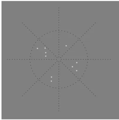
Fig. 1 caption. Which has the greater mean number of dots, the N1 = 8 occupied sectors on

the left or the N2 = 4 on the right? This is an example of the task faced by our observers,

except that the two stimuli were exposed (for 0.75 s) sequentially, rather than

simultaneously. In other versions of the task the number of occupied sectors in the two

stimuli were equal (N1 = N2 = 8 or N1 = N2 = 4). Occupied sectors alternated with unoccupied

sectors. The positions of the dots in each occupied sector varied randomly. An independent

sample from the binomial distribution with parameters ni and pi (i = 1, 2) determined the

number of dots in each occupied sector. For all stimuli, the number of binomial "trials" was

4, i.e. n1 = n2 = 4. The probabilities of binomial "success" (p1 and p2) were varied

systematically. We classified a response as 'correct' if observers selected the stimulus with a

higher value of pi. For further explanation see the text.

Each dot was a maximum-contrast, white Gaussian blob, with space constant σ = 2.2 pixels.

Its position within its sector was independently selected from a 4.7-pixel/side square, centred on one of the vertices (also selected at random, without replacement) of a notional 3x3-square grid, in which adjacent vertices were separated by 25 pixels. The grids

sector boundaries, as seen in Fig. 1. Each stimulus was exposed for 0.75 s, with a 0.5-s inter-stimulus interval. Observers selected from two keys on the keyboard to indicate which of the two stimuli had the greater mean number of dots per occupied sector. No feedback was provided.

Preliminary experiment

Before carrying out the main experiment we wished to convince ourselves that the number of dots in each separate sector could be counted accurately, irrespective of the number of dots in the other sectors (i.e. without crowding). To do this, we present only a single occupied sector in the first stimulus, containing 1, 2, or 3 dots. The second stimulus contained a variable number of occupied sectors. The observer was instructed to ignore everything except the previously occupied sector, and report whether it now contained the same number of dots, 1 more dot, or 1 fewer dot than in the first stimulus. These three possibilities were equally likely.

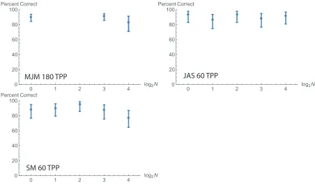
The results (Fig. 2) indicate consistently high performances, regardless whether the number of occupied sectors in the second stimulus was 1, 2, 4, or 8. Observers MJM and SM

performed slightly less well when every sector in the second stimulus was occupied. Due to this suggestion of crowding, we avoided using more than 8 occupied sectors (spatially alternating with unoccupied sectors, as in Fig. 1) in our main experiment. However, it must be noted that all observers made errors, even in the case where the second stimulus

contained only one occupied sector. (MJM's and SM's errors occurred most frequently when the first stimulus has the same number or 1 fewer dot than the second stimulus's target sector. JAS's errors were more evenly distributed across the three types of trial.) We do not know the reason for these imperfect performances, but they allow the firm conclusion that humans are not infallible when comparing the number of discrete elements in two sets,

even when neither set exceeds the subitizing range (Kaufman, et al., 1949).

Main experiment

dots, observers were never uncertain regarding the number of occupied sectors in any given session.

Fig. 2 caption. Results of the preliminary experiment. Three observers (MJM, JAS, and a naïve observer SM) decided whether a single dot cluster in the first of two sequentially presented stimuli contained the same number of dots, 1 more dot, or 1 fewer dot than the cluster in the corresponding position in the second stimulus. The vertical axis shows the probability of a correct response in any of these three conditions. The horizontal axis shows the number of clusters in the second stimulus on a logarithmic scale. TPP = trials per point. Error bars contain 95% binomial confidence intervals. For further explanation see the text.

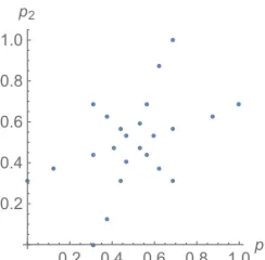
On each trial, the binomial probabilities of success {p1, p2} were selected randomly, without

replacement, from the 24-member set given in Fig. 3. Note this set contains just five

different values of Δp = |p1 – p2|. Eight members of this set have the property p1 + p2 < 1,

eight members have the property p1 + p2 = 1, and eight members have the property p1 + p2 >

1. On the basis of the first display it was impossible to guess (at a rate above 69 or 70%

correct, for N2 = 8 and N2 = 4, respectively) whether the second display would have a larger

or smaller average number of dots per occupied sectors.

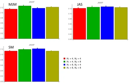
Performances are expressed as just-noticeable Weber fractions (JNWF; Solomon, et al.,

2011) in Fig. 4. On each trial, the Weber fraction (a physical quantity) can be defined as the ratio between sample means in the two stimuli, minus 1. To establish the JNWF (a

MJM 180 TPP

0 1 2 3 4 log2N

0 20 40 60 80 100 Percent Correct

0 1 2 3 4 log2N 0

20 40 60 80 100 Percent Correct

JAS 60 TPP

0 1 2 3 4 log2N

0 20 40 60 80 100 Percent Correct

psychophysical quantity), psychometric functions were formed, mapping log Weber fraction to the probability that observers selected the stimulus having the greater sample mean. We consider the standard deviation of the best-fitting (i.e. maximum likelihood) cumulative normal distribution to be the JNWF.

Fig. 3 caption. Binomial probabilities of success, {p1, p2}: {{0., 0.3125}, {0.125, 0.375},

{0.3125, 0.}, {0.3125, 0.4375}, {0.3125, 0.6875}, {0.375, 0.125}, {0.375, 0.625}, {0.40625, 0.46875}, {0.4375, 0.3125}, {0.4375, 0.5625}, {0.46875, 0.40625}, {0.46875, 0.53125}, {0.53125, 0.46875}, {0.53125, 0.59375}, {0.5625, 0.4375}, {0.5625, 0.6875}, {0.59375, 0.53125}, {0.625, 0.375}, {0.625, 0.875}, {0.6875, 0.3125}, {0.6875, 0.5625}, {0.6875, 1.}, {0.875, 0.625}, {1., 0.6875}}.

All JNWFs fall between 11 and 13%, which is within the normal range for standard numerosity discrimination (Ross, 2003; Annobile, Ciccini & Burr, 2014; Morgan, Raphael,

Tibber & Dakin, 2014). Differences between the conditions are small, but after Bonferroni

correction, 4 of the 18 (six per observer) pairwise comparisons, using the generalized likelihood ratio (Mood, Graybill, & Boes, 1974, pp. 440-441), suggested a significant

difference (i.e. –2 ln λ > 8.95), at the α = 0.05 level: MJM found 4/8 harder than 4/4 and 8/4 (i.e. his JNWFs were higher in the 4/8 condition) and SM found 8/4 harder than 4/4 and 8/8.

0.2 0.4 0.6 0.8 1.0p1 0.2

Fig. 4 caption. Just-noticeable Weber fractions in the main experiment, averaged over all

conditions except the four shown. N1 and N2 refer to the number of occupied sectors in the

first and second stimuli. Error bars represent 1 standard error. For further explanation see the text.

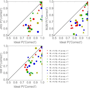
The data, separated by all 12 combinations of N1, N2 and the three probability conditions p1

+ p2 < 1, p1 + p2 = 1, and p1 + p2 > 1, are shown in Fig. 5. Each panel plots the performance (probability 'correct') of a human observer against the performance of the ideal observer, who uses all the patches in the stimulus to calculate the mean. Note that the ideal makes errors because the stimulus with the greater sample mean does not always correspond to

the binomial distribution with the greater expectation np. The data show that the human

observers are inefficient, particularly when there are 8 occupied sectors in one or both of

the stimuli. The red symbols, where N1 = N2 = 4, tend to be closer to the diagonal line,

indicating more efficient performance. The data for the naïve observer SM are closer to that of the ideal than either of the authors.

0.00 0.02 0.04 0.06 0.08 0.10 0.12

JNWF

0.00 0.02 0.04 0.06 0.08 0.10 0.12

JNWF

0.00 0.02 0.04 0.06 0.08 0.10 0.12

JNWF

N1=4,N2=4

N1=4,N2=8

N1=8,N2=4

N1=8,N2=8

MJM

JAS

Fig. 5 caption. Each panel plots the performance of one observer against the calculated performance of the ideal observer, in each of the 12 conditions. Perfectly efficient performance would fall along the diagonal. For further explanation see the text.

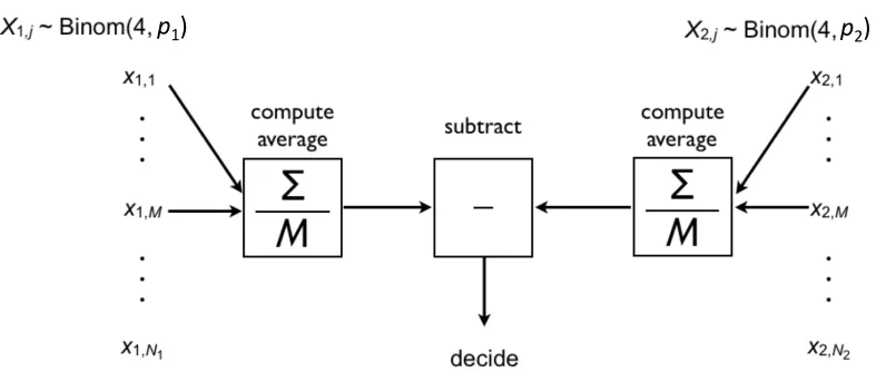
One potential source of inefficiency is subsampling: observers may ignore some of the occupied sectors when computing mean number. A model observer, for which subampling is the only source of inefficiency, is presented graphically in Fig. 6. In this model, the

observer randomly selects M of each stimulus's N occupied sectors when computing mean

number. Performance is limited by the fraction M/N, as well as by the stochastic element in

the initial binomial sampling. In the most general fit, we allowed the effective set-size M to

vary with each combination of N1 and N2. In the nested version, all four values of M were

forced to be identical.

Futhermore, all of our models allowed for the possibility of imperfect performances, even on the easiest of trials. Specifically, we assumed there would be some small proportion of

trials δ, on which observers completely ignored the stimulus and responded incorrectly. This

"lapse rate" was allowed to vary freely with each each combination of N1 and N2. Best-fitting

■ ■ ■■ ● ● ●● ▲ ▲ ▲ ▲ ■ ■ ● ● ● ▲ ▲ ▲▲ ■ ■ ● ● ● ▲ ▲ ▲ ■ ■ ● ● ● ▲ ▲ ▲ ▲

0.5 0.6 0.7 0.8 0.9 1.0 0.5 0.6 0.7 0.8 0.9 1.0

Ideal P('Correct')

JA S P ( 'Correct '

) ■● NN11==4,4,NN22==4,4,pp11++pp22=<11

▲ N1=4,N2=4,p1+p2>1

■ N1=4,N2=8,p1+p2<1

● N1=4,N2=8,p1+p2=1

▲ N1=4,N2=8,p1+p2>1

■ N1=8,N2=4,p1+p2<1

● N1=8,N2=4,p1+p2=1

▲ N1=8,N2=4,p1+p2>1

■ N1=8,N2=8,p1+p2<1

● N1=8,N2=8,p1+p2=1

▲ N1=8,N2=8,p1+p2>1

■ ■ ■ ■ ● ● ●● ▲▲ ▲ ▲ ■ ■ ● ● ●● ▲ ■ _● ■ ● ● ● ▲ ▲ ▲ ▲ ■ ■ ■ ■ ● ● ● ▲ ▲ ▲

0.5 0.6 0.7 0.8 0.9 1.0 0.5 0.6 0.7 0.8 0.9 1.0

Ideal P('Correct')

MJM

P

(

'Correct

'

) ■ N1=4,N2=4,p1+p2<1

● N1=4,N2=4,p1+p2=1

▲ N1=4,N2=4,p1+p2>1

■ N1=4,N2=8,p1+p2<1

● N1=4,N2=8,p1+p2=1

▲ N1=4,N2=8,p1+p2>1

■ N1=8,N2=4,p1+p2<1

● N1=8,N2=4,p1+p2=1

▲ N1=8,N2=4,p1+p2>1

■ N1=8,N2=8,p1+p2<1

● N1=8,N2=8,p1+p2=1

▲ N1=8,N2=8,p1+p2>1

■ ■ ■ ■ ● ● ● ● ▲ ▲ ▲ ▲ ■ ■ ■ ● ● ● ▲ ▲ ■ ■ ■ ● ● ● ● ▲ ▲ ▲ ■ ■ ■ ● ● ● ▲ ▲ ▲

0.5 0.6 0.7 0.8 0.9 1.0 0.5 0.6 0.7 0.8 0.9 1.0

Ideal P('Correct')

SM P ( 'Correct ' )

■ N1=4,N2=4,p1+p2<1 ● N1=4,N2=4,p1+p2=1 ▲ N1=4,N2=4,p1+p2>1

■ N1=4,N2=8,p1+p2<1

● N1=4,N2=8,p1+p2=1

▲ N1=4,N2=8,p1+p2>1 ■ N1=8,N2=4,p1+p2<1 ● N1=8,N2=4,p1+p2=1 ▲ N1=8,N2=4,p1+p2>1

■ N1=8,N2=8,p1+p2<1

● N1=8,N2=8,p1+p2=1

values never exceeded 0.043. (This latter value was estimated from the most-general fit of the subsampling model to SM's data from the 8/4 condition.) Note that this value is much lower than the 0.30 or 0.31 predicted for an otherwise-ideal observer who ignored the second of each trial’s two displays.

Fig, 6 Caption. Model of the subsampling, inefficient observer used to fit the data. There

were N1 occupied regions in the first interval and N2 in the second. However, in this model,

the observer computed the average of just M clusters in each interval, provided M clusters

were available. If there were fewer than M clusters, then observers used all the clusters. M

is the effective set size. The ratio of M to N is the efficiency with which the observer

computes each average. We fit this model to the data from each observer. In the most

general fit, we allowed the effective set-size M to vary with each combination of N1 and N2.

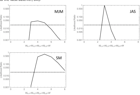
Fig. 7 shows the likelihood ratios (vertical axis) between the best fit of the most-general

model and the nested model, using the various values of M shown on the horizontal axis.

The dashed lines indicate the criterion likelihood ratio, below which the best fit of the nested model would be significantly worse than that of the most-general model (i.e. –2 ln λ > 7.81), at the α = 0.05 level. Since all of these curves contain points above this criterion ratio, we do not have compelling evidence for the effective sample size changing with

cluster numbers N1 and N2. Maximum-likelihood estimates for the effective sample size

varied between 3 (for our least-efficient observer JAS) and 5 (for most-efficient or nearest-to-the-ideal observer, SM).

Fig. 7 caption. Each of these panels shows the likelihood ratios between best fit of the

most-general model and a nested model, in which all four values of M were forced to be identical.

The dashed lines indicate the criterion likelihood ratio, below which the best fit of the nested model would be significantly worse than that of the most-general model. Since all of these curves contain points above this criterion ratio, we do not have compelling evidence

for the effective sample size changing with cluster numbers N1 and N2. Maximum-likelihood

estimates for the effective sample size varied between 3 (for our least-efficient observer JAS) and 5 (for most-efficient or nearest-to-the-ideal observer, SM). For futher explanation see the text.

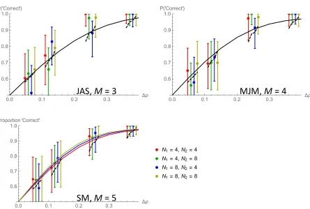
In Fig. 8 we compare human data with the best-fitting performances of two models. One (Fig. 6) that uses a fixed number of occupied sectors in its computations and an alternative

model (inspired by Raidvee, Lember, & Allik, 2017) that uses each sector with probability β <

1. Both models predict that performances should increase with Δp, and that the

psychometric function mapping Δp to performance should be steepest (and consequently

best constrain model parameters) when p1 + p2 = 1, so that is the condition we illustrate in

Fig. 8. The solid curves show the best fits based on M-values of 4 (MJM), 3 (JAS) and 5

(SM), these being the best fitting values from the likelihood analysis presented in Fig. 7. (Note that these M-values suggest that neither MJM nor JAS should enjoy an

0 2 4 6 8

0.001 0.005 0.010 0.050 0.100 0.500 1

M4,4=M4,8=M8,4=M8,8=M

Likelihood

Rat

io

JAS

0 2 4 6 8

0.001 0.005 0.010 0.050 0.100 0.500 1

M4,4=M4,8=M8,4=M8,8=M

Likelihood

Rat

io

MJM

0 2 4 6 8

0.001 0.005 0.010 0.050 0.100 0.500 1

M4,4=M4,8=M8,4=M8,8=M

Likelihood

Rat

io

improvement in performance when N exceeds 4. That is why there is only one solid curve in the top two panels.)

Fig. 8 caption. Human data, with fits of two inefficient-observer models. Each point

summarizes data from the trials in which p1 + p2 = 1. Error bars contain 95% binomial

confidence intervals. Solid curves illustrate the best fit of the subsampling model, in which

efficiency is given by the ratio M/N. Dashed curves illustrate the best fit of the probabilistic

model, in which efficiency is given by the probability (β) that each occupied sector is

considered in computations of the mean.

Dashed curves in Fig. 8 show the the best fits of the probablistic model, based on β

-values of 0.60 (MJM), 0.60 (JAS) and 0.61 (SM). This model predicts that the psychometric

slope necessarily increases with the number of occupied sectors. The data do not really support this prediction, and a comparison of maximum likelihoods favors the subsampling model for all 3 observers. Differences in the Bayesian Information Criterion varied between 8.8 (for MJM) and 27 (for SM).

Conclusion

We find that observers can discriminate between sectored textures, on the basis of the mean number of items per sector, with a respectable JNWF in the region of 12%; not very

0.0 0.1 0.2 0.3 Δp

0.6 0.7 0.8 0.9 1.0 P('Correct')

0.0 0.1 0.2 0.3 Δp

0.6 0.7 0.8 0.9 1.0 P('Correct')

0.0 0.1 0.2 0.3 Δp 0.6

0.7 0.8 0.9 1.0 Proportion 'Correct'

N1=4,N2=4

N1=4,N2=8

N1=8,N2=4

N1=8,N2=8

JAS,

M

= 3

MJM,

M

= 4

different from the values reported in previous studies of numerosity discrimination (e.g.

Ross, 2003; Anobile, Cicchini, & Burr, 2014; Morgan, et al., 2014). We conclude that number

can be averaged, just like size, orientation, and the spacing between texture elements. As in previously described cases of averaging, our observers perform this task with inefficiency. Their effective sample sizes (between 3 and 5) are significantly less than that (8) of the ideal observer.

The number of items per sector can be considered local density. Thus, it would be fair to describe our observers’ task as one of local-density discrimination. Consequently, our data suggest that the JNWF for local density is around 11–13%, regardless how many sectors are presented. Thus, it is the expected number of dots per sector that matters in our task; not the total number of dots.

Our findings add to the growing collection of evidence (e.g. Solomon, May, & Tyler, 2016) for a low limit on effective set sizes for summary statistics. However, it should be noted that our results do not imply that attention can be split amongst sectors. As suggested by

Myczek and Simons’s (2008) work, attention could have been deployed to each of 3–5

sectors sequentially. In fact, using an orientation-averaging task, Solomon, et al. found that

effective set sizes increased with display duration. However, they also found that some observers’ effective set sizes exceeded 1 even when display durations were sufficiently brief to make some of the stimuli effectively invisible. Exposures in our numerosity experiment were much longer than this, putatively providing enough time for several shifts of attention.

In general, our task is not equivalent to standard numerosity discrimination, because the observers have to take into account the number of occupied sectors in making their

decision. Specifically, in cases where N1 ≠ N2 our observers were effectively forced to

integrate information over a number (M in our subsampling model) of spatially distinct

regions, and then divide by that same number. However, it is possible that observers use the same strategy for dot counting, both in standard numerosity discrimination and in our

conditions where N1 = N2. The relative complexity of this operation may explain reports that

Acknowledgment

This research was originally reported at the 2016 meeting of the Society for Neuroscience.

References

Anobile G., Cicchini G.M., Burr D.C. 2014 Separate mechanisms for perception of numerosity and density. Psychological Science 25, 265-270.

Dakin, S.C. 2014 Seeing statistical regularities. In J. Wagemans (ed.) The Oxford Handbook of Perceptual Organization. New York: Oxford University Press.

Kaufman E.L., Lord M.W., Reese T.W., & Volkmann J. 1949 The discrimination of visual number. The American Journal of Psychology 62(4), 498-525.

Mood, A. M., Graybill, F. A., & Boes, D. C. (1974). Introduction to the theory of statistics. New York:McGraw-Hill.

Morgan M.J., Raphael S., Tibber M.S., & Dakin S.C. 2014 A texture-processing model of the 'visual sense of number'. Proceedings of the Royal Society of London. Series B: Biological Sciences 281, 20141137.

Myczek K., & Simons D.J. 2008 Better than average: Alternatives to statistical summary representations for rapid judgments of average size. Perception & Psychophysics 70, 772-288.

Raidvee A., Lember J., & Allik J. 2017 Discrimination of numerical proportions: A

comparison of binomial and Gaussian models. Attention, Perception, and Psychophysics79,

267–282.

Ross J. 2003 Visual discrimination of number without counting. Perception, 32(7), 867-870.

Solomon J.A., May K.M, & Tyler C.W. 2011 Inefficiency of orientation averaging:

evidence for hybrid serial/parallel temporal integration.
Journal of Vision, 16(1):13, 1-7.

Solomon J.A., Morgan M., & Chubb C. 2011
Efficiencies for the statistics of size