Rochester Institute of Technology
RIT Scholar Works
Theses
Thesis/Dissertation Collections
12-2014
Statistical Methods for Signal Processing with
Application to Automatic Accent Recognition
Zichen Ma
Follow this and additional works at:
http://scholarworks.rit.edu/theses
This Thesis is brought to you for free and open access by the Thesis/Dissertation Collections at RIT Scholar Works. It has been accepted for inclusion in Theses by an authorized administrator of RIT Scholar Works. For more information, please [email protected].
Recommended Citation
Master’s Thesis
Statistical Methods for Signal
Processing with Application to
Automatic Accent Recognition
Author:
Zichen Ma
Supervisor:
Dr. Ernest Fokou´e
A thesis submitted in partial fulfillment of the requirements
for the degree of Master of Science in Applied Statistics
in the
The John D. Hromi Center for Quality and Applied Statistics
The Kate Gleason College of Engineering
Committee Approval
The undersigned have examined thesis titled “Statistical Methods for Signal Processing with Application to Automatic Accent Recognition” by ZichenMa, a candidate for the
degree of Master of Science in Applied Statistics, and hereby approve that it is worthy of acceptance:
Dr. Ernest FOKOU ´E Date
Thesis advisor, associate professor, Center for Quality and Applied Statistics
Dr. Joseph VOELKEL Date
Committee member, professor, Center for Quality and Applied Statistics
Dr. Steven LALONDE Date
Committee member, associate professor, Center for Quality and Applied Statistics
I, ZichenMa, declare that this thesis titled, “Statistical Methods for Signal Processing
with Application to Automatic Accent Recognition” and the work presented in it are my own. I confirm that:
This work was done wholly or mainly while in candidature for a research degree
at this University.
Where any part of this thesis has previously been submitted for a degree or any
other qualification at this University or any other institution, this has been clearly stated.
Where I have consulted the published work of others, this is always clearly
at-tributed.
Where I have quoted from the work of others, the source is always given. With
the exception of such quotations, this thesis is entirely my own work.
I have acknowledged all main sources of help.
Where the thesis is based on work done by myself jointly with others, I have made
clear exactly what was done by others and what I have contributed myself.
Signed:
Date:
“We balance probabilities and choose the most likely. It is the scientific use of the
imagination.”
Abstract
The Kate Gleason College of Engineering Master of Science
Statistical Methods for Signal Processing with Application to Automatic
Accent Recognition
by ZichenMa
The problem of classification of people based on their phonetic features of accents is posted. This thesis intends to construct an automatic accent recognition machine that can accomplish this classification task with a decent accuracy. The machine consists of two crucial steps, feature extraction and pattern recognition. In the thesis, we review and explore multiple techniques of both steps in great detail. Specifically, in terms of fea-ture extraction, we explore the techniques of principal component analysis and cepstral analysis, and in terms of pattern recognition, we explore the algorithms of discriminant function, support vector machine, and k-nearest neighbors. Since signal data usually exhibit the feature of High Dimension Low Sample Size, it is crucial in the automatic accent recognition task to reduce the dimensionality.
Acknowledgements
I am especially grateful to my thesis advisor Dr. Ernest Fokou´e for his teaching of all the concepts and notions that are extremely useful in the completion of this research work. I enjoyed every single conversation with him and have learned so much through these conversations. I will remember for my life his enthusiasm, patience, and kindheartedness in sharing his beautiful knowledge and experience with me.
I wish to thank Dr. Steven LaLonde and Professor Joseph Voelkel for their kindly acceptance of being in my thesis committee and their precious advises to my research. I wish to sincerely thank the John D. Hromi Center for Quality and Applied Statistics for accepting me as a student in the master’s program and paying part of my tuition. I would also thank every single faculty and staff member in the department for their teach and help in the past two years.
I would like to thank Mr. Kyle Sauln and Ms. Sara Smacher for their help in the voice collection and all the participants for their generous participation.
I would give my deepest thanks to my parents, who are always supporting me in ac-complishing this master’s degree overseas in the United States, which is an opportunity that they never dreamed of for themselves.
Last, this thesis is typed and edited in LATEX.
Committee Approval i
Declaration of Authorship ii
Abstract iv
Acknowledgements v
Contents vi
List of Figures ix
List of Tables x
1 Introduction 1
1.1 Motivation and problems . . . 1
1.2 Background: Signal processing . . . 2
1.2.1 Signal and signal processing . . . 2
1.2.2 Speech processing and its subfields . . . 3
1.2.3 Continuous-time and discrete-time signals . . . 4
1.2.4 Signal as big data of HDLSS variety . . . 4
1.2.5 Graphical representations of signal . . . 5
1.3 Background: Statistical learning . . . 5
1.3.1 Learning problems . . . 5
1.3.2 Supervised learning . . . 6
1.3.3 Learning problems in the HDLSS context . . . 7
1.4 Aim of the thesis . . . 7
1.5 Thesis organization . . . 8
2 Techniques in Feature Extraction 10 2.1 Principal component analysis . . . 11
2.1.1 Classical PCA . . . 11
2.1.2 PCA on dual space . . . 12
Contents vii
2.2.1 Pre-emphasis and finite impulse response . . . 14
2.2.2 Window function and short time Fourier transform . . . 15
2.2.3 Filter banks and mel-scale . . . 17
2.2.4 Computation of MFCCs . . . 20
3 Statistical Classification 21 3.1 Binary classifier . . . 22
3.1.1 Discriminant function . . . 22
3.1.2 Support vector machine . . . 24
3.1.3 K-nearest neighbors . . . 26
3.2 Cross-validation. . . 28
3.2.1 K-fold cross-validation and confusion matrix . . . 29
3.2.2 Hold-out method and stratified sampling . . . 30
4 Implementation of Automatic Accent Recognition - Study and Results 32 4.1 The First Study. . . 32
4.2 Analysis on Time Domain . . . 33
4.2.1 Dimension Reduction . . . 35
4.2.2 Comparison of classifiers . . . 36
4.2.3 How many PC’s to keep? . . . 37
4.3 Analysis on frequency domain . . . 38
4.3.1 Predictive performance . . . 38
4.3.2 Computational performance . . . 41
4.4 Further Discussion . . . 44
5 Implementation of Automatic Accent Recognition - Effect of Noise 45 5.1 Continuation of the first study . . . 45
5.1.1 Perturbing signal with noise. . . 45
5.1.2 Predictive performance on noisy data . . . 46
5.2 The second study . . . 47
5.2.1 Description of the study . . . 47
5.2.2 Analysis on frequency domain. . . 49
5.3 Further Discussion . . . 50
6 Conclusion 52 6.1 Performance of accent recognition machine . . . 52
6.1.1 Time or frequency?. . . 52
6.1.2 Which classifiers to use? . . . 52
6.1.3 When does it fail? . . . 53
6.2 Future work . . . 53
A Selected R Code 55 A.1 R Code in Performing Analysis on Time Domain . . . 55
List of Figures
1.1 Block diagram of the recognition task . . . 1
1.2 Waveform and spectrogram . . . 6
2.1 Pre-emphasis . . . 15
2.2 Fourier decomposition . . . 16
2.3 Generalized Hamming window . . . 17
2.4 Effect of Hamming window . . . 18
2.5 Relation between mel-scale and hertz-scale. . . 19
2.6 Filter bank . . . 19
3.1 Linear optimal hyperplane in SVM . . . 24
3.2 Nonlinear optimal hyperplane in SVM . . . 25
3.3 Discrepancy between training error and test error . . . 28
4.1 Comparison of waveforms . . . 34
4.2 Histogram of length of amplitude vectors . . . 34
4.3 Plot of the eigenvalues . . . 35
4.4 Test error on time domain . . . 37
4.5 Percent variation vs. mean prediction accuracy . . . 38
4.6 Comparison of spectrograms. . . 39
4.7 Comparison of prediction accuracy on frequency domain . . . 40
4.8 Relative prediction accuracy on frequency domain . . . 41
4.9 Computational time for feature extraction . . . 42
4.10 Comparison of computational time of classifiers . . . 42
4.11 Relative computational time. . . 43
5.1 Noise with different levels of amplitude . . . 46
5.2 Mean prediction accuracy with noisy data . . . 48
5.3 A speech signal in the second study. . . 49
3.1 Confusion matrix . . . 29
4.1 Summary of study . . . 33
4.2 Number of Principal Components . . . 36
4.3 Training performance on time domain . . . 36
4.4 Predictive performance on frequency domain . . . 40
5.1 Predictive performance with noisy data . . . 47
5.2 Predictive performance in the second study . . . 50
For my father
Introduction
1.1
Motivation and problems
Our work is mainly motivated by a question in the field of signal processing: can peo-ple be statistically grouped into different classes by their accent features of some spoken
language? In such questions, several points should be drawn attention to. First, we are solely interested in the features at the stage of phonetics, not involving any seman-tics analysis. In linguisseman-tics, phoneseman-tics is the study of the sounds of the speech whereas semantics involves the study of the meaning of the speech ([Hayes, 2010], [Johnson, 2003]). That is to say, we are to perform the classification based only on the sounds, not taking care of what the speech exactly is. Second, such classification should be per-formed through statistical methods. Though other methods can be used to accomplish the classification, mainly in linguistics ([Biadsy,2011]), our work focuses on the statis-tical methods. Third, a basis of “some spoken language” should be chosen upon which different accents can be compared to each other. In this research, the basis is English, or more specifically, American English.
Following the logical idea of this question, it is of interest to analyze the statistical clas-sification of people according to their accents of speaking English. Figure 1.1 gives an abstract block diagram of such automatic accent recognition. The recognition task is
Figure 1.1: A block diagram of the automatic accent recognition task
achieved through a set, or rather, a chain of machines. Starting from some raw input speeches, some feature extraction techniques are used to extract the useful phonetic
Chapter 1. Introduction 2 features in the speech, and then the features are sent to some pattern recognition ma-chines, that is, some classification techniques, to accomplish the classification. At last, the outputs are the classes, usually represented by a set of integer indices.
Thus, the general question posted in the beginning boils down to the following specific questions:
• How are we to perform the feature extraction?
• How are we to perform the pattern recognition?
• If there are multiple techniques that can be chosen at each stage, is there a best one? If so, which combination of techniques should be preferred?
• Is the predictive performance of such combination of techniques in feature extrac-tion and pattern recogniextrac-tion consistently stable?
Combining the above specific questions together, the goal of our research is indeed:
Given a set of speech signals in English, construct an automatic accent
ma-chine that classifies speakers into different classes of accents. For instance, in
the sense of binary classification, we can group the speakers into two categories that indicate if they have American accent.
1.2
Background: Signal processing
1.2.1 Signal and signal processing
In [Priemer,1991], a signal is defined as “a function that conveys information about the behavior or attributes of some phenomenon.” Such information may include but not limit to audio, video, speech, image, conversation, music. Physically, any vibration over time or over space would create signals. If the quantity exhibits vibration over time, it generates any kinds of patterned audio signals, while a vibration over space would create image signals.
Signal processing is an area of study that deals with the analysis of signals. In [ Op-penheim and Schafer,1975], the authors dated the start of signal processing back to as early as 17th century, while they also claimed that the modern signal processing started from 1940s.
• Audio processing: The study of electrical signals that represent sound.
• Image processing: The study of signal processing in which the input is image.
• Video processing: The study of video signals, especially movies.
• Array processing: The study of signals from arrays of sensors.
In this thesis, the word “signal” only means the vibration over time or simply audio signal. Also, although noise is often defined as random disturbance of signal, in this thesis we sometimes use the word “signal” as the mixture of pure signal and noise for simplicity.
1.2.2 Speech processing and its subfields
As a subfield of signal processing, speech signal processing, or speech processing for short, deals with speech signals and its process. That is, the input signals are human speech. Speech processing has risen as an important area in the sense that it is closely related to natural language processing and artificial intelligence in general ([Boves and de Vethd, 1996], [Liu and Hansen, 2010], [Hardcastle and Laver, 1999]). Though all intend to perform the analyses based on speech signals, its subjects usually exhibit some substantial differences. Below is a list of some of the subfields in speech processing ([Nerbonne,2003]).
• Speech recognition: The study that deals with the translation between signal and text.
• Speaker recognition: The study that deals with the identification of specific speak-ers based on speech signals.
• Dialect recognition: The study of recognizing the dialect of the object of a speech signal.
• Accent recognition: The study of recognizing the accent of the object of a speech signal.
Chapter 1. Introduction 4 pronunciation. Thus, dialect recognition involves analysis in both phonetics and seman-tics, but usually accent recognition only involves phonetics. For instance, the sentences “He has British accent” and “He speaks British dialect” convey slightly different mean-ings. In terms of analysis, accent recognition is often text-independent while dialect recognition is usually text-dependent.
1.2.3 Continuous-time and discrete-time signals
Signals can be categorized in various ways ([Huang et al., 2001]). In terms of time, signals can be categorized into:
• Continuous-time signal: any real-valued function that is defined at a continuous timet in a finite or infinite interval.
• Discrete-time signal: a function that maps from integers, representing discrete time, to any real numbers. In this sense, a signal is simply a time series.
Intuitively, continuous-time signals are real signals that come from speech, telephone, or other sources. Usually, discrete-time signals are obtained through sampling from continuous-time signals using digital devices. Most of the time the signals being used for analysis are discrete-time signals or rather digital signals.
1.2.4 Signal as big data of HDLSS variety
As stated above, the signals in research analyses are usually discrete-time signals and are collected from sampling. It is of great importance to recognize that signal becomes “big data” due to this sampling procedure. A sampling rate is defined as the number of samples being taken from the signal per unit time, usually in seconds ([Shannon,1949]). That is, how frequent it is to draw a sample from the continuous signal. To preserve most of the information from the signal, it is crucial to keep this frequency as a relatively large number. For instance, if we are to sample a signal with a sampling rate of 8,000 Hz, that is, to draw 8,000 samples from the signal per second, a 10-second digital signal would contain 80,000 elements in it. For most recording devices, a sampling rate of 44,100 Hz or 48,000 Hz is considered as moderate.
researches in signal processing exhibit the feature of High Dimension Low Sample Size (HDLSS).
Formally, an n×pdata matrix X exhibits the form below.
X=
x11 x12 · · · x1p
x21 x22 · · · x2p
..
. ... ... ... ...
xn1 xn2 · · · xnp
.
It is said to be HDLSS if np.
1.2.5 Graphical representations of signal
So far, a question should be asked naturally: What exactly is sampled from the signal?
Or, in terms of time series,what indeed does the time series consist of ? Usually on time domain, the signal is a time series of amplitude, the instant loudness of the signal at the time being collected. It is always helpful to present the signals graphically. In general, there are two types of graphical representations that are commonly used:
• Waveform: a time series plot of the amplitude of a signal.
• Spectrogram: a visual representation of the frequency of a signal. That is, how much of a signal at each time period lies on each of the frequency bands.
As a crucial term, “frequency” shall be introduced in Chapter 2. Figure 1.2 gives a comparison of waveform and spectrogram of a male voice speaking the word “approx-imation”. Notice that the waveform is rather simple, and the spectrogram is much more complex and interesting, in which the X-axis represents time, Y-axis represents frequency, and the shade on the graph represents how much energy there is at each period of time and each band of frequency.
1.3
Background: Statistical learning
1.3.1 Learning problems
Chapter 1. Introduction 6
0.0 0.2 0.4 0.6
−0.20
−0.05
0.10
Time (sec)
Amplitude
0.0 0.1 0.2 0.3 0.4 0.5 0.6
0
5000
15000
time
[image:19.596.134.495.103.346.2]frequency
Figure 1.2: A male voice speaking “approximation”, represented in waveform and spectrogram
general that almost any question that has been discussed in statistical science has its analogue in learning theory.” Rather, in [Turing, 1950], Alan Turing intended to de-fine machine learning by proposing the general question: Can machines do what we (as thinking entities) can do?
1.3.2 Supervised learning
In general, learning problems can be categorized into two classes, supervised learning and unsupervised learning, based on the availability of the knowledge of the target ([Vapnik, 1995]). These two types of problems can be defined as:
• Supervised learning: the type of learning problems that seeks to find the pattern between the independent variables (or features) and the known dependent variable (or target)y.
• Unsupervised learning: the type of learning problems in which there is no already known target.
learning simply because there is a known target that is being regressed on. Without this crucial piece of knowledge, such analysis can never be established on (especially when the target is continuous.)
In detail, the solution of a supervised problem consists of three parts ([Vapnik,1995]):
• Some data that consist of feature vectorsx.
• A target y that contains the output of every feature vectorx.
• A learning machine that contains a set of functions which ultimately achieves the mapping from input space to output space.
Specifically, if the targety is discrete and contains the indices that indicate the distinct class to which the feature vectorsxbelong, such supervised learning problems are called classification. In such case, the learning machine is usually called a classifier.
1.3.3 Learning problems in the HDLSS context
In the context of data that exhibit HDLSS feature, learning problems are sometimes difficult to deal with, mainly because such problems are not well-posed. According to [Hadamard,1923], a well-posed problem should have the following properties:
• A solution exists.
• The solution is unique.
• The solution’s behavior changes continuously with the initial conditions.
The violation of any one of the above properties would cause the problem to deteriorate to an ill-posed problem. Thus, an important task in this research is to seek some methods through which the ill-posed problems can be transformed into well-posed problems.
1.4
Aim of the thesis
Our research intends to give insights in the following:
Chapter 1. Introduction 8 domain-specific technique of feature extraction performs better than the general technique since it reduces the dimensionality of the data and in the mean time extracts more meaningful features.
• Classification: We demonstrate the difference of classifiers in performing the clas-sification task through some procedures of model validation.
• Robustness of the performance: We also examine if the predictive performance is affected significantly by noise. That is, when there is evident amount of noise, would the accent recognition machine still perform relatively convincing prediction results or degrade quickly?
1.5
Thesis organization
In order to thoroughly convey the idea and results of our research, the thesis consists of 6 chapters, with this chapter being the first and presenting an introduction to the topic and a brief background of the context of the research.
Chapter 2 and 3 can be considered as Part One, in which some theory and facts are reviewed. Chapter 2 reviews techniques in feature extraction. We start with the gen-eral technique of principal component analysis and elaborate the situation in which the data matrix exhibit high dimension low sample size feature so that the classical prin-cipal analysis is infeasible and an alternative should be preferred. Then we move on to a domain-specific technique of feature extraction, namely, the cepstral analysis. We thoroughly work through the steps following which the computation of a useful type of feature, the mel-frequency cepstral coefficients, is performed.
Chapter 3 explores some basic concepts in statistical classification. We first review three types of binary classifiers, through which the features are able to be classified into distinct classes. Although the techniques are aiming at the same goal of accomplishing the classification, we intend to illustrate the differences of these techniques.
Chapter 4 and 5 can be considered as Part Two, in which the experiments and results that represents the performance of the implementation of automatic accent recognition are presented. Chapter 4 starts with the description of the first experiment, in which the pure signals were collected, and continues to the analysis in time domain and frequency domain based on this dataset.
Chapter 2
Techniques in Feature Extraction
This chapter reviews two alternative methods in feature extraction, principal component analysis (PCA) and cepstral analysis. PCA can be performed in the time domain, while cepstral analysis is naturally implemented on frequency domain. Both techniques have the advantage of reducing dimensionality together with feature extraction.
Section 2.1 reviews the technique of principal component analysis. Though normally considered as a method of remedying multicollinearity, and thus of reducing dimension-ality, PCA essentially achieves the goal of feature extraction via orthogonal transform. Typically, the principal components can be obtained through eigenvalue decomposition of XTX and orthogonal transformation, where X is the data matrix, but this is not achievable when the data exhibits structure of high dimension and low sample size, as is usually encountered in signal processing. In the latter case, PCA has to be performed in terms of the dual space XXT.
Section 2.2 reviews the method of cepstral analysis, a powerful tool for feature extraction, specifically designed for signal processing. Starting from some pre-processing work on time domain, the signal is transformed onto frequency domain. And the goal is to extract a type of feature called mel-frequency cepstral coefficients (MFCCs) via nonlinear mapping and discrete cosine transform. The MFCC vectors are orthogonal to each other, and by controlling how many vectors to preserve, we can control the dimensionality of the input.
2.1
Principal component analysis
2.1.1 Classical PCA
As one of the most important applications in linear algebra and possibly one of the most influential multivariate statistical learning techniques, principal component analy-sis can be dated back to [Pearson,1901], or, as its modern formalization, to [Hotelling, 1933], who also created the termprincipal component. Its goal is to answer the following question: For a dataset that contains possibly inter-correlated variables, can we obtain another dataset that is the linear combination of the original basis and that re-expresses
the data optimally? ([Abdi and Williams, 2010]) Given a large dataset that contains numerous variables, the problem of multi-collinearity, that is, variables are heavily cor-related to each other, is almost always inevitable. Thus it is not meaningful to preserve the original dimensionality. Principal component analysis helps to reduce the high di-mensionality and to reveal the feature of the data.
Specifically, let Xn×p be a given dataset that contains n observations and p variables
and n > p. Each of the column vectorxi in the matrix Xn×p = [x1,x2, . . . ,xp]
is a random variable with mean E(X) and finite variance. Thus the covariance matrix Σ can be written as
Σ = E
h
(X−E[X])T(X−E[X])
i
.
If we assume thatxi’s are centered at 0, the equation above can be simplified to
Σ = EXTX.
And the corresponding sample covariance matrix is
S= 1
n−1
xT1x1 xT1x2 · · · xT1xp xT2x1 xT2x2 · · · xT2xp
..
. ... . .. ...
xT
px1 xTpx2 · · · xTpxp
.
Chapter 2. Feature Extraction 12 problem is to re-construct a datasetZof which the covariance matrix is in fact diagonal, that is, the covariance between any two variables is exactly 0. It can be shown that this optimal solution is indeed the eigenvalue decomposition of the matrix XTX ([Johnson and Wichern,2007]).
Based on the well-known theorem from linear algebra that any square symmetric matrix can be orthogonally (orthonormally) diagonalized, we have
XTX=UΛUT (2.1) whereU is a p×p orthogonal matrix of which the column vectors are the eigenvectors and Λ = diag(λ1, λ2, . . . , λp) is the diagonal matrix of which the diagonal entries are
the eigenvalues.
Given the eigen-pairs [(λ1,u1),(λ2,u2), . . . ,(λp,up)], where λ1 ≥ λ2 ≥ · · · ≥ λp ≥ 0,
each elementzijin thejth principal componentZjcan be written as a linear combination
of the column vectors in the original data matrix.
zij =xTi uj,i = 1,2, . . . ,n,j = 1,2, . . . ,p. (2.2)
An important fact of this decomposition is that the sum of the eigenvalues equates to the trace of the matrix being decomposed, that is,
p
X
i=1
λi=trace(XTX)
and notice again that the trace is simply the sum of variance of the variables, that is, the total variance. Thus, based on the magnitude of the eigenvalues, it is often not necessary to preserve all p principal components. If, given a positive number q < p, the last (p−q) eigenvalues are relatively small and we can arbitrarily conclude that those variables essentially contribute very little to the total randomness of the data, it is natural that we only preserve the first q principal components, or the important information, and thus achieve the task of dimension reduction ([Johnson and Wichern, 2007]).
2.1.2 PCA on dual space
observations is smaller than the number of variables,XTXis not of full rank any more, or, in some extreme cases when the ratio between n and p is extremely small, the matrix cannot even be estimated computationally. Thus, the regular PCA cannot be performed in such situation. Fortunately, it has been shown that PCA is achievable in terms of the dual spaceXXT ([Shen et al.,2013], [Yata and Aoshima,2010]).
We start from the fact that the matrices XTX and XXT share the same non-zero eigenvalues ([Strang,2009]). Notice that in Equation2.1, the matrixU is orthonormal, that is,U−1U=UTU=I, whereI is the identity matrix. Thus, we have
XTXU=UΛUTU=UΛ. (2.3) Then by pre-multiplying both sides of Equation 2.3 by X and using Equation 2.2, we have
XXTXU=XUΛ
and
XXTZ=ZΛ.
Zis ann×p matrix with independent columns, andΛis a p×pdiagonal matrix with
nnon-zero eigenvalues. The eigenvalues of zero’s contribute nothing to the performance of PCA. Thus, we can keep the non-zero part of matrix Λ, which is the top-left n×n
block, and truncate off the other parts. For matrixZ, we only keep the first n columns and truncate all the followingn−p columns. This truncation gives
XXTV=VΛD,
where V and ΛD are the truncated matrices of Zand Λ. Also notice that columns in V are uncorrelated, thusV is invertible, which leads to
XXT=VΛDV−1. (2.4)
Equation2.4indicates that instead of dealing with matrixXTX, we can perform eigen-value decomposition on the dual matrixXXTand obtain the component scores directly
from matrix V ([Jung and Marron,2009], [Jung,2011]).
2.2
Cepstral analysis
Chapter 2. Feature Extraction 14 to map the transformed signal in hertz onto Mel-scale due to the fact that 1 kHz is a threshold of humans’ hearing ability. Human ears are less sensitive to sound with frequency above that threshold. Cepstral analysis is considered a powerful algorithm in fields such as speaker recognition ([Tivari, 2010], [Hasan et al., 2004], [Hanani, 2012], [Chen and Luo, 2009]) and musical instrument analysis ([Logan, 2000], [Sturm et al., 2010]). The calculation of MFCCs includes the following steps:
• Pre-emphasis filtering
• Take the absolute value of the short time Fourier transformation using windowing
• Warp to auditory frequency scale (Mel-scale)
• Take the discrete cosine transformation of the log-auditory-spectrum
• Return the first q MFCCs
2.2.1 Pre-emphasis and finite impulse response
Letx[n] be a discrete signal, wherenis the index. Before the signalx[n] is transformed to frequency domain or is passed to any formal analysis, it is usually necessary to consider some preliminary analysis, especially when the signal contains an evident background noise. Finite impulse response (FIR) filter is one of these techniques. Usually, a finite impulse response filter is defined as
s[n] =b0x[n] +b1x[n−1] +· · ·+bNx[n−N]
=
N
X
i=0
bi·x[n−i],
where x[n] is the input signal and s[n] is the output. Notice that FIR filter can be considered as a smoothing technique over a finite time period N given some conditions on the coefficients bi. Specifically, the first-order FIR filter
s[n] =x[n] +αx[n−1] (2.5) is called pre-emphasis and can be determined as a high-pass filter or a low-pass filter based on the value of α. When α > 0, it is a low-pass filter, which means that low frequency is emphasized while high frequency is de-emphasized. It is a high-pass filter when α <0 and the high frequency is emphasized in this situation.
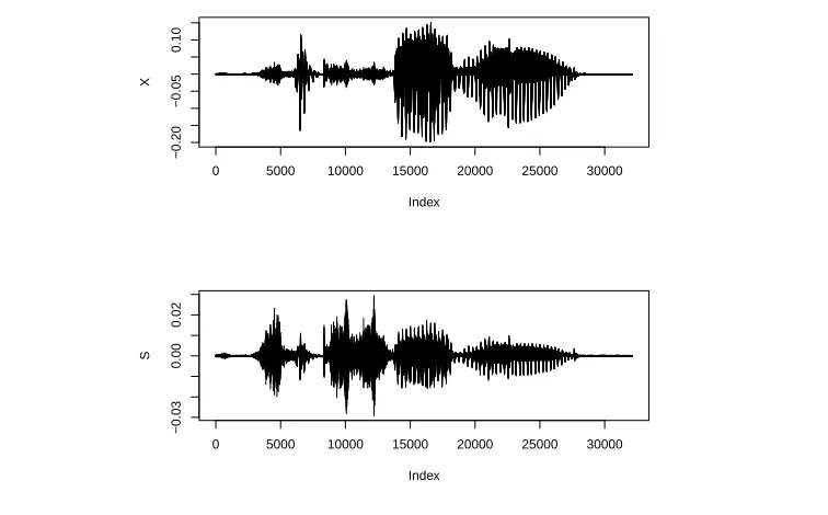
is important as a preliminary process due to the fact that the signal-to-noise ratio (SNR) is lower at low frequency. By emphasizing the high frequency band and de-emphasizing the low frequency band, the pre-emphasis filter is in fact boosting the signal. Figure2.1 shows the effect of pre-emphasis. Notice that the voice portion of the signal is boosted while the non-voice portion, or the transition part between voice portions, is damped.
0 5000 10000 15000 20000 25000 30000
−0.20
−0.05
0.10
Index
X
0 5000 10000 15000 20000 25000 30000
−0.03
0.00
0.02
Index
[image:28.596.130.508.198.433.2]S
Figure 2.1: The effect of pre-emphasis withα=−0.95
2.2.2 Window function and short time Fourier transform
Named after the French mathematician Joseph Fourier (1822), Fourier transform has been playing an important role in signal processing in the sense that it is the crucial link between time domain and frequency domain. Given a periodical but not necessarily sinusoidal signal function over time, such as a piece of music or speech, the goal is to represent this signal by some pure sinusoidal functions, that is, sine and cosine waves. Specifically, given a signal function f(x), the Fourier transform can be written as
ˆ
f(ξ) =
Z ∞ −∞
f(x)e−2πjxξdx, for any real number ξ,
where j is the complex unit. When the independent variable x represents time with unit of seconds, the transform variable ξ represents frequency in hertz. The transform utilizes the Euler’s formula
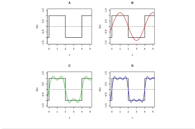
Chapter 2. Feature Extraction 16 and thus we have a integration of sine and cosine waves with different frequencies. Figure 2.2 gives an intuitive idea of Fourier transform. The waveform in panel A is called a
0 1 2 3 4 5
−1.5 −0.5 0.5 1.5 A x f(x)
0 1 2 3 4 5
−1.5 −0.5 0.5 1.5 B x f(x)
0 1 2 3 4 5
−1.5 −0.5 0.5 1.5 C x f(x)
0 1 2 3 4 5
[image:29.596.122.509.131.387.2]−1.5 −0.5 0.5 1.5 D x f(x)
Figure 2.2: Fourier decomposition of a square wave
square wave. Using Fourier transform, it can be decomposed into the sum of different sinusoidal waves. From panel B to panel D, we add two, three, and four sine waves together, and the approximation is more similar to the true square wave.
An important assumption of Fourier transform is that it assumes that the signal is stationary, but this assumption can hardly hold when the signal is relatively long. Al-though the amplitude over time is exactly centered at 0 due to the sampling procedure, its variance may vary a lot at different time. This flaw can be remedied by implementing short-time Fourier transform, which states that a signal over a very short time is nearly stationary. Mathematically, it is given by
Xa[k] = Lw−1
X
n=0
s[n]·wa[n]·e−j2πkn/Lw = Lw−1
X
n=0
s[n]·wa[n]·e−jωk,0≤k < Lw (2.6)
wherewa[n] is the window function being utilized as a method to truncate a long signal
into short pieces, andLw is the length of the window. By definition, a window function
Hamming window is given by
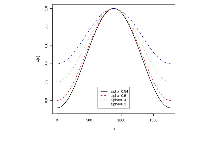
w[n] = (1−α)−α cos
2πn Lw−1
,0≤n < Lw (2.7)
and when α = 0.54, it is the traditional Hamming window, named after Richard Ham-ming, and whenα = 0.5, it is a Hanning window, named after Julius von Hann. Figure 2.3 generalized Hamming window with different values of α. Notice that all the
func-0 500 1000 1500
0.0
0.2
0.4
0.6
0.8
1.0
n
w[n]
[image:30.596.133.500.230.469.2]alpha=0.54 alpha=0.5 alpha=0.4 alpha=0.3
Figure 2.3: Generalized Hamming window with differentα
tions approach 1 in the center while die down toward 0 at the end. If we are to break the signal into short pieces, an overlap between pieces is necessary and this die-down pattern is crucial to keep the consistency of the signal. Figure 2.4 illustrates the effect of a traditional Hamming window. The ends of the windowed signal are approaching 0 by multiplying the window function and s[n] together. Usually the window length is chosen to be around 40 milliseconds, with an overlap of around 10 milliseconds between the consecutive windows to keep the continuity of the whole signal.
2.2.3 Filter banks and mel-scale
Chapter 2. Feature Extraction 18
0 10 20 30 40
−0.04
0.00
0.04
Time(ms)
x
0 500 1000 1500
0.2
0.6
1.0
n
w[n]
0 10 20 30 40
[image:31.596.128.511.91.345.2]−0.03 0.00 0.02 Time(ms) Windo wing
Figure 2.4: The effect of a Hamming window
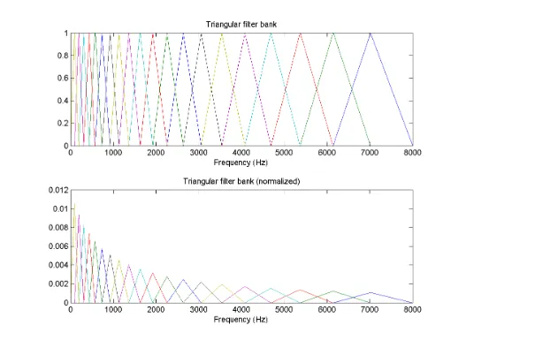
triangular filter of lengthLf can be written as
Mm[k] = 1−
k−Lf−1 2
Lf−1 2
,0≤k < Lf (2.8)
We can assign the filter bank linearly to a signal on frequency domain, that is, to arrange the filters in a way such that every filter covers a frequency band with the same length. Yet this method is not efficient enough on a hertz scale since the hearing ability of human is more sensitive to the frequency band from 20 to 1000 hertz. Thus it is less efficient to assign the same length to a filter at higher frequency as to a filter at lower frequency. Fortunately, the mel-scale, named by Stevens, Volkman, and Newman (1937), compensates this problem through a nonlinear mapping between hertz-scale and mel-scale using logarithm. This transform can be done by
mel=
f f ≤1000
2595 log101 +700f f >1000
(2.9)
0 10000 20000 30000 40000
0
1000
2000
3000
4000
Hertz−Scale
[image:32.596.153.503.137.388.2]Mel−Scale
Figure 2.5: The transform between mel-scale and hertz-scale is a nonlinear mapping
[image:32.596.184.495.495.696.2]Chapter 2. Feature Extraction 20 again that as the frequency increases, the filters would cover a wider band. And again a short length of overlap is necessary to keep the continuity.
2.2.4 Computation of MFCCs
Now we can perform the final computation of MFCCs with the help of filter banks and mel-scale. First, we can compute the log-energy for each filter, which is written as
S[m] = ln
"N−1 X
k=0
|xa[k]|2Mm[k]
#
,0< m≤M (2.10)
Notice that within the summation sign, we multiply the energy and the filter together to perform the grouping of feature.
Finally, the mel-frequency cepstral coefficients are given by the discrete cosine transform of the above output:
c[q] =
M−1
X
m=0
"
S[m] cos πq(m−
1 2)
M
!#
,0< m≤M (2.11) Some points should be drawn attention to. First, we can arbitrarily control the numberq
to decide how many coefficients to preserve. In practice, this number is usually between 12 and 40. Second, for a complete signal, the output of MFCCs is an Nw ×q matrix
where Nw is the number of windows and q is the number of MFCCs. In order to
Statistical Classification
This chapter reviews some basic concepts in statistical classification. In statistics and machine learning, classification is the problem that categorize a new observation into one of the several classes based on some knowledge of training data and their observed classes. In this sense, classification is a supervised learning problem, and it is significantly different from cluster analysis, which is an unsupervised learning problem that attempts to group similar observations into the same cluster without the help of some training data of which the true classes are known. The most common, or intuitive problems in classification are binary problems, where the target is of only two classes. In this case, the data shall be passed to a classifier, an algorithm or machine that performs the classification. Section 3.1 reviews some of the binary classifiers. After the model is fitted from a training set, it is always of interest to examine if the the model has a decent prediction ability. Such examination can be somewhat fulfilled through cross-validation, which will be reviewed in Section 3.2.
In Section 3.1, we go over three different binary classifiers, namely, discriminant function, support vector machine, and k-nearest neighbors. It is of importance to know that all of these algorithms can perform classification for multi-categories, but in this chapter they are introduced only in the binary context. Also, though some classifiers are more robust than the others theoretically, to decide which classifier is the best or the most useful in a specific task is more empirical.
Section 3.2 reviews cross-validation, a crucial technique in checking if the model has strong prediction ability. In this section, we compare the commonK-fold algorithm and the hold-out method. In the binary classification sense, random sampling is usually not reasonable, thus an alternative method, stratified sampling, is introduced.
Chapter 3. Statistical Classification 22
3.1
Binary classifier
3.1.1 Discriminant function
A standard approach to supervised classification problems is the discriminant analysis. From a Bayesian perspective, let Y ∈ {1,2, . . . , K} be a discrete target and X be the data matrix. The binary classification problem can be proposed like this: given some featurexi, classify the corresponding targetyi into one of the classes. A straightforward
and rather reasonable strategy is to classify yi into the most probable class given the
data ([James et al.,2013]). Formally, the problem can be written as ˆ
f(x) = max
k P r(Y =k|X=x).
The target function at the right-hand side is a conditional probability and it is directly related to the famous Bayes’ Theorem. Given two events A and B, the conditional probability P r(B|A) is given by
P r(B|A) = P r(A|B)·P r(B)
P r(A) , or simply expresses in words as
Posterior∝Likelihood·Prior.
Intuitively, it states that our knowledge of some fact (that is, the prior) can be updated (that is, the posterior) through taking into account the data (that is, the likelihood). Invoking this well-known theorem, the posterior probability being maximized can be re-written as the following
P r(Y =k|X=x) = fk(x)πk
f(x) ,
where fk(x) is the conditional density ofx in class k, πk the prior probability of
corre-sponding classk, andf(x) the marginal density ofX. Thus the discriminant analysis is a likelihood-based technique. That is, in order to compute the posterior probability, it is necessary to have some knowledge of the distribution offk(x).
A common assumption when such knowledge is insufficient is to assign the likelihood a Gaussian distribution. That is to write the likelihood as
fk(x) = (2π)−p/2|Σk|−1/2exp
−1
2(x−µk)
TΣ−1
k (x−µk)
Sometimes the marginal distribution of X is difficult to compute, but with the help of a standard trick in Bayesian inference, we can get rid of the denominator completely since it is constant regardless of which classyi is in. Thus, we can specify the posterior
probability as proportional to the product of the likelihood and the prior probability.
P r(Y =k|X=x)∝fk(x)·πk
= (2π)−p/2|Σk|−1/2exp
−1
2(x−µk)
TΣ−1
k (x−µk)
·πk.
Since maximizing the above equation is the same as maximizing the logarithm of it, given the fact that the logarithm function is always monotonic, the above equation can be rearranged as
δk(x) =−
1
2log|Σk| − 1
2(x−µk)
TΣ−1
k (x−µk) +log(πk). (3.1)
Without further assumptions, Equation3.1is usually called the quadratic discriminant function, since it is a quadratic form in terms of x ([Hastie et al.,2013]). The decision rule is to assign xto classi ifδi(x)> δj(x), that is,
ˆ
fQDA(x) = arg max
k δk(x) (3.2)
A further assumption that specifies the same covariance matrix to all classes is sometimes applied. That is, the covariance matrices can be written as Σ1 = Σ2 =· · ·= ΣK = Σ.
Under such condition, Equation 3.1can be further simplified to
δk(x) =xTΣ−1µk−
1 2µ
T
kΣ
−1µ
k+log(πk). (3.3)
Chapter 3. Statistical Classification 24
3.1.2 Support vector machine
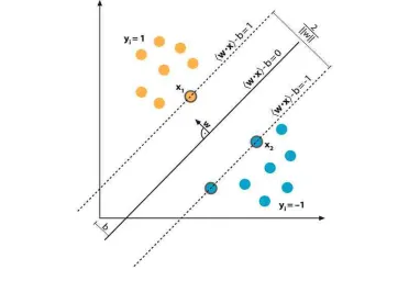
Ever since its invention in [Cortes and Vapnik,1995], support vector machine has been demonstrated as the state-of-the-art technique in binary classification. In its simplest case, in which there exists a linear decision boundary, or a hyperplane, that can com-pletely separate the data of two classes. SVM deals with the question of what a best separation of the data should be. It concludes that the best separation is the solution of an optimization problem that seeks to maximize the distance between any observations and the linear boundary ([Clarke et al.,2009]).
Mathematically, a hyperplane on a p-dimensional space can be defined as
w·x−b= 0 (3.4) where w is a coefficient vector, x is a point on the p-dimensional space and b is a constant. For a dataset D={(xi, yi)|xi ∈Rp, yi ∈ {−1,1}}ni=1, the optimal separating
[image:37.596.123.505.370.626.2]hyperplane is shown on Figure 3.1. Specifically, observations lying on the dot lines
Figure 3.1: The optimal hyperplane is shown as a solid line.
this minimization is the same as to minimize kwk2. Thus, this problem formalization
can be written as
arg min
(w,b)
1 2kwk
2
subject to: yi(w·xi−b)≥1.
The constant 12 in the target function is merely for mathematical simplicity. It can be shown that the above optimization problem can be solved through quadratic program-ming and the decision boundary of SVM is given by
ˆ
fSV M(x) =sign
X
i
ˆ
αiyixTi x+ ˆb
!
(3.5)
where ˆα and ˆb are the estimated coefficients. Notice that in the summation sign, the features appear in terms of inner products.
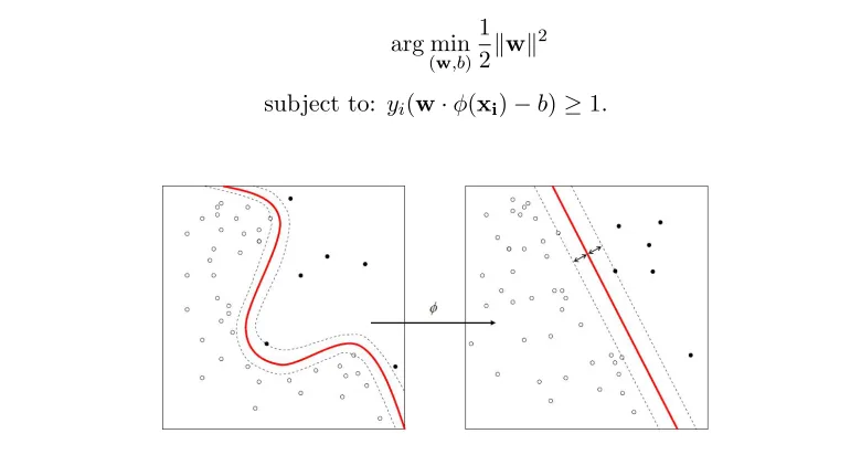
Further, if the data is not separable in the linear case but can be mapped to linear separation through a function φ, as is shown in Figure 3.2, the optimization problem has to be modified to
arg min
(w,b)
1 2kwk
2
[image:38.596.119.509.395.601.2]subject to: yi(w·φ(xi)−b)≥1.
Figure 3.2: The decision boundary in the nonlinear separable case.
It is obvious that in order to have a linear solution to the problem, the functionφmust transform the data to a higher dimension. The general SVM decision boundary is simply to replace the xvectors into a function φ(x).
ˆ
fSV M(x) =sign
X
i
ˆ
αiyiφ(xi)·φ(x) + ˆb
!
Chapter 3. Statistical Classification 26 It is of extreme importance to notice that the nonlinear mapping function φ appears in the decision function in the sense of feature space inner product. Computationally, choosing the functionφcan become infeasible quickly, while the well-known kernel trick should be used to avoid the explicit use ofφ. Assume a kernel functionK can be found so thatK(xi,x) =φ(xi)Tφ(x), the above decision boundary can be modified by replacing
the inner product to the kernel function. ˆ
fSV M(x) =sign
X
i
ˆ
αiyiK(xi,x) + ˆb
!
(3.7) This provides great convenience in which it is not necessary to compute the nonlinear mapping explicitly, but only to perform it implicitly through the kernel. Specifically, one can readily verify that Equation 3.5is simply a special case of Equation 3.7with a linear kernelK(xi,x) =xTi x. Some common kernel functions include the Radial Basis
Function (RBF) kernel
K(xi,x) =exp(−γ kxi−xk2)
and the polynomial kernel
K(xi,x) = (xi·x+c)d.
It is also of importance to know that there is no theoretical proof showing one kernel function is significantly better than others, so that which kernel function to use is an empirical practice and is usually decided through the comparison of prediction accuracy of SVM models using different kernels.
3.1.3 K-nearest neighbors
Comparing to the above two techniques, the algorithm of k-nearest neighbors is more intuitive and is often considered as a lazy learning. The idea of this algorithm states like this: given a dataset with known classes, or simply put, a training set, and some new data points with unknown classes, compare the distance of a new point and its first k nearest neighbors and assign the new point to the class that majority of these neighbors lie within. For instance, whenk= 1, we simply assign a new data point to the same class as its single nearest neighbor ([Fokou´e,2013]). That it is considered as a lazy learning is because no formal model is needed in this algorithm. The only requirements are a dataset in which the classes of observations are already known, some measurement for distance, and an integerk.
Mathematically, let T r ={(xi, yi)|xi ∈ Rp, yi ∈ {1,2,· · ·, S}}ni=1 be a training set and
x∗ a new data point. The distances of x∗ and xi’s are computed by based on some
{xi|D(x∗,xi) ≤ D(k)}, where D(k) is the distance between the new point and the kth
nearest neighbor. And the decision boundary can be written as ˆ
fkN N(x∗) = arg max j∈{1,2,···,S}{
1
k
n
X
i=1
I(yi=j)I(xi∈ Vk(x∗))} (3.8)
whereI(·) is an indicator function.
The crucial part of k-NN algorithm is the distance function. Conventionally, the Eu-clidean distance
D(xi,xj) =
v u u t
n
X
l=1
(xil−xjl)2
or the Manhattan distance
D(xi,xj) = n
X
l=1
|xil−xjl|
are commonly used in the computation. Also, in binary classification,k is usually chosen to be an odd integer simply to avoid the tie-up situation. The pseudo-code of k-nearest neighbors algorithm is given below.
Begin
• Input: T r = {(xi, yi)|xi ∈ Rp, yi ∈ {1,2,· · ·, S}}ni=1 as the training set and
x∗ a new data point.
• Order D(x∗,xi) from lowest to highest.
• Select the k nearest observations tox∗,Vk(x∗).
• Assign to x∗ the most frequent class in Vk(x∗).
End
A problem of this algorithm arises when the data contain significant amount of noise. That is, if there is significant noise in the training set and there are some outliers in each class, the results of classification using k-NN would degrade. Thus in this sense, k-NN is not a robust algorithm. Some substantial work has been done to remedy this drawback. Also, the algorithm of k-nearest neighbors suffers the curse of dimensionality. That is, when the dimensionality increases, the predictive performance of this algorithm would drastically degenerates.
Chapter 3. Statistical Classification 28 lowest prediction risk one can obtain, and the the risk R that is given by the nearest neighbor algorithm, it has been proven that asymptotically
R≤2R∗ (3.9) as number of observationsnapproaches infinity. The Inequality3.9states that regardless of its simple algorithm, the prediction risk would not exceed two times of the lowest risk.
3.2
Cross-validation
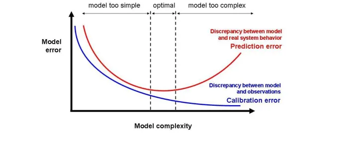
[image:41.596.152.506.490.632.2]For models that are used to provide prediction rather than some explanation, it is always necessary to assess the model fit in the sense of prediction accuracy. When a model is fitted to some data, there are two types of prediction, the in-sample prediction, in which the model is tested on the same data that were used to fit it, and the out-of-sample prediction, in which the model is tested on some other data. The corresponding errors are called training error (or calibration error) and test error (or prediction error). Shown in the Figure 3.3, as the model complexity increases, the training error would always decrease and even approach 0, while the test error behaves as a V-shape. Thus the training error would cause a false optimism for a relatively complex model. Invented in Stone (1951), cross-validation intended to remedy the false optimism. The idea of cross-validation is to construct a model based only on one random portion of the dataset and validate the prediction accuracy on the other portion.
3.2.1 K-fold cross-validation and confusion matrix
There are many different methods to perform cross-validation, but the most common one is the K-fold cross-validation algorithm ([James et al.,2013], [Clarke et al.,2009]). Given a random sample, the algorithm follows the procedure below:
Begin
• Randomly divide the sample into K equal portions.
• For i= 1,2, . . . , K, hold out portion i and fit the model from the rest of the data.
• For i= 1,2, . . . , K, use the fitted model to predict the holdout sample.
• Average the measure of predictive accuracy over the K different fits.
End
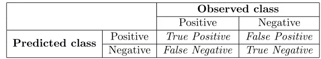
[image:42.596.156.472.515.574.2]Different from prediction in regression, the prediction error in classification, especially in binary classification, is easy to tell: a prediction error occurs only when the predicted class is different from the true, or the observed, class. Thus for a binary classification, in which the target is only of two classes, positive and negative, the results can be arranged in a confusion matrix, as is the one shown below, which is a two-by-two table showing the relationship between the predicted values and the observed values.
Table 3.1: A general 2×2 confusion matrix
Observed class
Positive Negative
Predicted class Positive True Positive False Positive
Negative False Negative True Negative
The cells of the table are the counted numbers and they are defined below.
• True Positive (TP): The situation that the predicted class and the observed class are both positive.
• False Positive (FP): The situation that an observation is predicted as positive but observed as negative.
Chapter 3. Statistical Classification 30
• True Negative (TN): The situation that the predicted class and the observed class are both negative.
Thus, it is obvious that the prediction accuracy (ACC) is the sum of diagonal elements over the total number of observations and the prediction error is simply the complement of accuracy.
ACC= T P +T N
T otal
3.2.2 Hold-out method and stratified sampling
Sometimes when we do not have the luxury of large number of observations, it is not feasible to make the number K of folds very large. In such case, a hold-out method of cross-validation is usually preferred and its procedure is as follows:
Begin
• Randomly divide the sample into 2 portions, a training set containing roughly 70% of the observations, and a test set containing the rest 30% of the data.
• Fit the model from the training set.
• Use the fitted model to predict the test set, and compute the predictive accu-racy.
• Iterate the above steps m times and average the predictive accuracy of each iteration as the mean predictive accuracy (MPA).
End
Begin
• Perform random sampling within each class. That is, sample 70% of the observations from each class as training sets and preserve the rest.
• Combine the two training sets as a whole training set. Do the same to the test set. Thus, the total observations being used in the training test is still 70%.
• Fit the model from the training data and predict the test data, and compute the predictive accuracy.
• Iterate the above steps m times and average the predictive accuracy of each iteration as the mean predictive accuracy.
End
Finally, the mean predictive accuracy (MPA) can be expressed as
M P A=
Pm
i=1ACCi
Chapter 4
Implementation of Automatic
Accent Recognition - Study and
Results
This chapter implements the recognition techniques being reviewed in Chapter 2 and Chapter 3 through a designed study. Section 4.1 describes this study in detail. In Section 4.2, the accent recognition is performed on time domain. Section 4.3 intends to achieve the same goal on frequency domain.
4.1
The First Study
In order to implement the automatic accent recognition machine and to examine the prediction ability of the algorithm, an study was constructed and the signal data are collected in the study. The procedure of the study follows the steps below:
• Through an internet resource, 22 different voices are chosen, of which 11 are of American English accent and 11 are not. Of the non-American voices, there are 3 British English voices, 2 Spanish voices, 2 French voices, 2 Italian voices, and 2 German voices.
• Each voice is required to read 15 different multi-syllable English words, such as “approximation” and “beneficial”. These words were sampled randomly without replacement from a population of such words without replacement, which means that no words was assigned to two or more voices.
• A total of 15×22 = 330 soundtracks were recorded through some internal recording device with a sampling rate of 44,100 Hz.
[image:46.596.230.402.233.306.2]At this stage, we would not want the signals to be contaminated by noise, so that we used the internet resource together with internal recording device. Thus, the soundtracks only contained pure signals with the synthesized voices. A demographic summary of the soundtracks is given in Table 4.1.
Table 4.1: A demographic summary of soundtracks
Accent Gender
Female Male Total US 90 75 165 Non-US 90 75 165 Total 180 150 330
Notice that this study is balanced in terms of accent but imbalanced in terms of gender. Since this work only focuses on the recognition of different accents, we would ignore the gender of each voice at this point. Though each soundtrack only contain 1 single word and thus it is fairly short, with a sampling rate of 44,100 Hz, each one of the signal vectors contains more than 30,000 elements on time domain.
And based on the description above, the target, or response, of this classification problem is given by
yi =
−1 if non-US, 1 if US,
which defines this problem as a binary classification in which we are interested in cate-gorizing different voices into two distinct accent classes.
4.2
Analysis on Time Domain
Before the formal analysis, we would like to perform some brief preliminary analysis. Figure4.1is a graph containing the waveform of two signals of the same word “approx-imation”. The top panel is of British accent and the bottom panel American accent. Though it is of linguistics interest to dissect the waveforms further and to theorize some semantic features, we would not draw our attention on such analysis. Instead, we could readily conclude that it is infeasible to deduce the distinction of different accents solely based on the waveforms on time domain.
Chapter 4. Study & Results 34
0.0 0.5 1.0 1.5
−0.4
0.0
0.2
Time
Amplitude
0.0 0.5 1.0 1.5
−0.3
−0.1
0.1
Time
[image:47.596.139.507.102.346.2]Amplitude
Figure 4.1: A comparison of British accent (top) and American accent (bottom) in waveform
naturally have a variation. Figure4.2is a histogram of lengths of the amplitude vectors.
Dimensionality
Frequency
30000 40000 50000 60000
0
5
10
15
20
25
30
35
Figure 4.2: A histogram of length of amplitude vectors
[image:47.596.146.508.462.698.2]8955. From Figure4.2, it seems that the mode length is between 45000 and 47500, but even at its shortest length, which is below 30000, the dimension is still considered fairly high.
4.2.1 Dimension Reduction
As was discussed before, we would consider implementing PCA as the method of dimen-sion reduction on time domain, but as a matrix-based technique, PCA requires ann×p
feature matrix rather than n separate vectors with different lengths. Thus, we start by forming the data matrixX. The procedure is rather simple. Letpi be the length of each
vector, i= 1,2, . . . , n, then the dimensionality of the matrix p is
p= max{pi}, i= 1,2, . . . , n
For all the shorter vectors, the signals are duplicated until all p dimensions are fitted, but since the ends of a signal usually damp down, the duplicated part is essentially filled with 0.
Then we perform PCA on this data matrix following the idea shown in Section 2.1. Figure4.3illustrates the pattern of the eigenvalues, shown on the left-hand-side Y-axis, and the cumulative variation being explained by the first q eigenvalues, shown on the right-hand-side Y-axis. Though it is obvious that the eigenvalues are decreasing while the
0 50 100 150 200 250 300
0
200
400
600
800
1000
1200
0
20
40
60
80
100
Eigen
v
alue
Cum
ulativ
e P
ercent
[image:48.596.174.486.489.723.2]Eigenvalue Cumulative percent
Chapter 4. Study & Results 36 cumulative variation increases, it is difficult to tell how many principal components being preserved would be optimal. We would discuss this question in the following subsection, but at this stage, we follow one convention and preserve 95% of the variation. Table4.2 gives a portion of the eigenvalues and the corresponding cumulative variation.
Table 4.2: Number of Principal Components
# PC Eigenvalue Percentage (%) 206 75.3270 89.94 207 74.9464 90.08
..
. ... ... 249 52.0964 94.97 250 51.8996 95.07
From the table, if we are to preserve 95% of the total variation, the corresponding number of principal components to be kept is 250. Evidently, this number is significantly smaller than 67,072, and yet the transformed data matrix is still not of a satisfactory shape, considering the ratio between n = 330 and p = 250 is merely 1.32. Regardless, we are able to perform classification based on this matrix.
4.2.2 Comparison of classifiers
[image:49.596.220.412.177.273.2]We start by training three types of classifiers, discriminant function, SVM, and k-NN, using the full dataset. For discriminant analysis, only linear discriminant analysis can be performed, since there is not enough information to estimate two covariance matrices if we are to use quadratic discriminant function. For SVM, we use three different kernels, namely, the linear kernel, the RBF kernel, and the 2nd order polynomial kernel. For k-NN, the number of neighborskis chosen to be 3 based on a preliminary analysis using cross-validation. The results of training accuracy and error are given in Table 4.3.
Table 4.3: Summary of Training performance on time domain
Method Error (%) Accuracy (%) LDA 7.88 92.12 SVM-L 0.31 99.69 SVM-RBF 4.55 95.45 SVM-P 0 100
k-NN 24.85 75.15
the procedure stated in Section 3.2, we perform the hold-out algorithm with stratified sampling. The number of iterations m is set to be a moderate 500. The pattern of prediction accuracy is shown in the Figure 4.4. Each one of the boxes in the plot represents 500 estimated prediction accuracies.
● ● ● ● ● ● ● ● ● ● ● ● ● ● ● ● ● ● ● ● ● ● ● ● ● ● ● ● ● ● ● ● ● ● ● ● ● ● ● ● ● ● ● ● ● ● ● ● ● ● ● ● ● ● ● ● ● ● ● ● ● ● ● ● ● ● ● ● ● ● ● ● ● ● ● ● ● ● ● ● ● ● ● ● ● ● ● ● ● ● ● ● ● ● ● ● ● ● ● ● ● ● ● ● ● ● ● ● ● ● ● ● ● ● ● ● ● ● ● ● ● ● ● ● ● ● ● ● ● ● ● ● ● ● ● ● ● ● ● ● ● ● ● ●
LDA SVM−L SVM−RBF SVM−P k−NN
[image:50.596.193.429.185.394.2]0.35 0.40 0.45 0.50 0.55 0.60 0.65 T est Accur acy
Figure 4.4: A comparison of test error on time domain
It is obvious that none of the classifiers has convincing prediction ability. Regardless, it seems that SVM with RBF kernel is slightly better than the other classifiers. Further, comparing the training accuracies in Table 4.3 and the test accuracy, we can readily notice the discrepancy, which is likely caused by the overfitting issue. Also, for k-NN algorithm, most values of test accuracy are exactly 0.5. This is because of the degeneration of the algorithm. When an algorithm like this completely fails to perform, the two classes would collapse into a single class. And since the design of this study is balanced, exactly one half of the data would be falsely classified into the other category to which they should not belong.
4.2.3 How many PC’s to keep?
Chapter 4. Study & Results 38 done. We find an alternative method with the help of cross-validation. Assuming that we want to preserve at least 50% of the variation, we can plot the empirical relationship between the percentage of total variation and the mean prediction accuracy. Figure4.5 is one such plot based on the SVM-RBF classifier.
● ● ● ● ● ●● ● ●● ● ● ● ● ● ● ●● ● ● ● ● ●● ● ● ●● ● ● ● ● ● ● ● ● ● ● ● ● ● ● ● ● ● ● ● ● ●
50 60 70 80 90 100
[image:51.596.144.506.180.423.2]0.54 0.55 0.56 0.57 0.58 0.59 Cumulative Percent Mean Predictiv e Accur acy
Figure 4.5: The cumulative percent variation vs. mean prediction accuracy
From the plot, we can readily notice that preserving 95% of the variation is actually an inferior choice. Instead, it seems that MPA peaks when only around 60% or 70% of the total variation is kept. However, the peak MPA is still merely around 59%.
4.3
Analysis on frequency domain
Again, we start by some informal analysis. Figure4.6 gives the corresponding compar-ison of spectrogram as Figure 4.1. And still we are not able to deduce the difference between the accents of the two groups of people although we are given significantly more information than in the waveforms, regardless of the potential meaning in the spectrogram.
4.3.1 Predictive performance
0.0 0.5 1.0 1.5
0
10000
20000
time
frequency
0.0 0.2 0.4 0.6 0.8 1.0 1.2 1.4
0
10000
20000
time
[image:52.596.132.506.105.347.2]frequency
Figure 4.6: A comparison of British accent (top) and American accent (bottom) in spectrogram
through cepstral analysis. In detail, we examine the prediction ability of the classifiers with different numbers of MFCCs, varying from as small as 12 to as large as 39. The number of filters in the filter bank is chosen to be 40 in order to extract rich informa-tion from the signal. In terms of classificainforma-tion, we apply linear discriminant funcinforma-tion, quadratic discriminant function, SVM with linear, RBF, and 2nd order polynomial ker-nels, and k-NN. Table 4.4 provides the performance results on frequency domain. In each cell, the first value represents the training accuracy, the second value (initalic) the mean prediction accuracy, and the third value (in parenthesis) the standard deviation of the prediction accuracy.
Notice that although the training accuracy still exhibits overfitting, the prediction ac-curacy improves tremendously comparing to the performance on time domain. A corre-sponding plot of MPA values in Table 4.4is given below. Notice that the performances of LDA and SVM with linear kernel are close to each other and are both inferior than the other classifiers. K-NN demonstrates a better prediction ability, regardless of the number of MFCCs being used. Also, it is of interest to see that there is a relatively big improvement from 12 MFCCs being used, which simply indicates p = 12, to p = 26, and yet this improvement slows down from p= 26 to p = 39. For some classifiers, the accuracy even drops down slightly from p= 33 top= 39.
Chapter 4. Study & Results 40
Table 4.4: The predictive performance on frequency domain of the first study
# MFCCs LDA QDA SVM-L SVM-RBF SVM-P k-NN
12
0.7606 0.8394 0.7758 0.9000 0.9788 0.9424
0.7353 0.8112 0.7608 0.8208 0.8097 0.8548
(0.0362) (0.0329) (0.0351) (0.0374) (0.0364) (0.0306)
19
0.7818 0.9061 0.8152 0.9485 1.0000 0.9667
0.7503 0.8647 0.7734 0.8507 0.8851 0.9098
(0.0345) (0.0298) (0.0336) (0.0356) (0.0274) (0.0262)
26
0.8636 0.9697 0.8667 0.9758 1.0000 0.9758
0.8063 0.9224 0.8056 0.9080 0.9379 0.9398
(0.0322) (0.0262) (0.0337) (0.0278) (0.0227) (0.0217)
33
0.8970 0.9879 0.9212 0.9848 1.0000 0.9909
0.8319 0.9543 0.8399 0.9352 0.9509 0.9586
(0.0314) (0.0183) (0.0333) (0.0248) (0.0205) (0.0185)
39
0.8970 0.9879 0.9152 0.9758 1.0000 0.9909
0.8260 0.9383 0.8226 0.9223 0.9438 0.9605
(0.0332) (0.0219) (0.0326) (0.0247) (0.0216) (0.0178)
●
●
●
●
●
15 20 25 30 35 40
0.65 0.70 0.75 0.80 0.85 0.90 0.95 1.00 # MFCCs Accur acy ● ● ● ● ● ● ● ● ● ● ● ● ● ● ● ● ● ● ● ● ● ● ● ● ● LDA QDA SVM−L SVM−RBF SVM−PLY k−NN
[image:53.596.127.510.385.694.2]number of MFCCs and illustrates the relative relationship of the classifiers. While the
●
● ● ●
●
15 20 25 30 35 40
[image:54.596.150.506.129.372.2]−0.2 −0.1 0.0 0.1 # MFCCs Accur acy ● ● ● ● ● ● ● ● ● ● ● ● ● ● ● ● ● ● ● ● ● ● ● ● ● LDA QDA SVM−L SVM−RBF SVM−PLY k−NN
Figure 4.8: A comparison of relative prediction accuracy on frequency domain
algorithm of k-NN is considered as the best algorithm in this case, SVM with linear kernel and LDA are constantly below average performance, which is somewhat reasonable since both classifiers try to accomplish linear classification.
4.3.2 Computational performance
Chapter 4. Study & Results 42 ● ● ● ● ● ● ● ● ● ● ● ● ● ● ● ● ● ● ● ● ● ● ● ● ● ● ●
15 20 25 30 35
[image:55.596.163.508.104.343.2]8.50 8.55 8.60 8.65 8.70 8.75 #MFCCs Time F or F eature Extr action (sec)
Figure 4.9: The computational time being used for feature extraction
At the stage of pattern recognition, the question in terms of computation is: which classifier accomplishes the task with the least time? Figure 4.10 ill