Comparison of different iterative schemes for ISPH based on Rankine source solution

City, University of London Institutional Repository

Citation

:

Zheng, X., Ma, Q. and Duan, W.Y. (2017). Comparison of different iterative

schemes for ISPH based on Rankine source solution. International Journal of Naval

Architecture and Ocean Engineering, 9(4), pp. 390-403. doi: 10.1016/j.ijnaoe.2016.10.007

This is the published version of the paper.

This version of the publication may differ from the final published

version.

Permanent repository link: http://openaccess.city.ac.uk/18493/

Link to published version

:

http://dx.doi.org/10.1016/j.ijnaoe.2016.10.007

Copyright and reuse:

City Research Online aims to make research

outputs of City, University of London available to a wider audience.

Copyright and Moral Rights remain with the author(s) and/or copyright

holders. URLs from City Research Online may be freely distributed and

linked to.

City Research Online:

http://openaccess.city.ac.uk/

[email protected]

Comparison of different iterative schemes for ISPH based on Rankine

source solution

Xing Zheng

*

, Qing-wei Ma

, Wen-yang Duan

a

College of Shipbuilding Engineering, Harbin Engineering University, Harbin 150001, China

b

Schools of Engineering and Mathematical Science, City University, London EC1V 0HB, UK

Received 3 June 2016; revised 17 October 2016; accepted 23 October 2016 Available online 28 December 2016

Abstract

Smoothed Particle Hydrodynamics (SPH) method has a good adaptability for the simulation of free surface flow problems. There are two forms of SPH. One is weak compressible SPH and the other one is incompressible SPH (ISPH). Compared with the former one, ISPH method performs better in many cases. ISPH based on Rankine source solution can perform better than traditional ISPH, as it can use larger stepping length by avoiding the second order derivative in pressure Poisson equation. However, ISPH_R method needs to solve the sparse linear matrix for pressure Poisson equation, which is one of the most expensive parts during one time stepping calculation. Iterative methods are normally used for solving Poisson equation with large particle numbers. However, there are many iterative methods available and the question for using which one is still open. In this paper, three iterative methods, CGS, Bi-CGstab and GMRES are compared, which are suitable and typical for large unsymmetrical sparse matrix solutions. According to the numerical tests on different cases, still water test, dam breaking, violent tank sloshing, solitary wave slamming, the GMRES method is more efficient than CGS and Bi-CGstab for ISPH method.

Copyright©2016 Society of Naval Architects of Korea. Production and hosting by Elsevier B.V. This is an open access article under the CC BY-NC-ND license (http://creativecommons.org/licenses/by-nc-nd/4.0/).

Keywords:SPH; ISPH; ISPH_R; Iterative scheme; Dam breaking; Violent tank sloshing; Solitary wave slamming

1. Introduction

With the development of numerical methods, meshless particle methods get the robust advantage for breaking waves and their interaction with marine structures in naval archi-tecture and ocean engineering. There are many different meshfree methods, such as Smoothed Particle Hydrodynamics (SPH) method (Monaghan, 1994), Moving Particle Semi-implicit (MPS) method (Koshizuka and Oka, 1996; Zhang et al., 2006; Khayyer and Gotoh, 2011), Meshless Local Petrov-Gelerkin (MLPG) method (Ma and Zhou, 2009) and so on. SPH is arguably one of most often-used meshfree methods and has been widely applied in marine and ocean engineering (Oger et al., 2007; Xu et al., 2009; Lind et al., 2012; Rafiee

et al., 2012; Colagrossi and Landrini, 2003; Liu and Liu, 2006; Schwaiger, 2008; Ferrand et al., 2013; Zheng et al, 2014). There are two SPH schemes. One is weakly compressible SPH and the other is incompressible SPH (ISPH). The latter one is based on the time project method and need to solve the Poisson equation, which also meets the problems of large sparse matrix solution. There are many applications of ISPH method for water wave simulations (Rafiee et al., 2012; Lind et al., 2012; Xu et al., 2009; Shao and Lo Edmond, 2003; Shao et al., 2006; Shao, 2009) as it performs betters in many cases.

The principle of ISPH is to solve the partial differential equation for the pressure through the projection method. The project method was firstly implemented to the SPH method by

Cummins and Rudman (1999). Many researchers have also improved and modified the projection method to make it more accurate and efficient. Compared to WCSPH, ISPH is a typi-cally implicit by dealing with the pressure and velocity as *Corresponding author.

E-mail address:[email protected](X. Zheng).

Peer review under responsibility of Society of Naval Architects of Korea.

ScienceDirect

Publishing Services by Elsevier

International Journal of Naval Architecture and Ocean Engineering 9 (2017) 390e403

http://www.journals.elsevier.com/international-journal-of-naval-architecture-and-ocean-engineering/

http://dx.doi.org/10.1016/j.ijnaoe.2016.10.007

primitive variables. WCSPH can be easy to program (Shadloo et al., 2012) and it is more widely used at present. However, some researcher (Hu and Adams, 2007;Xu et al., 2009; Zheng et al., 2014) suggested that ISPH was more accurate especially in the pressure representation. The reason is that when handling fluid flow with larger Reynolds number (typically

>100), the standard WCSPH method has be found to suffer from large density variations. Hu and Adams (2007), Ellero et al. (2007) and Zheng et al. (2014) pointed out that WCSPH was computationally less efficient than ISPH in the case of fluids with different numerical cases.

With the improvement of ISPH method, some key numer-ical technologies are applied.Xu et al. (2009)andLind et al. (2012) introduced a fick shift method to avoid the particle pattern distribution. Bonet and Lok (1999), Khayyer et al. (2008) proposed a corrected kernel formulation of the pres-sure gradient calculation, which can improve the accuracy of first derivative computing. In order to improve the pressure distribution,Zhang et al. (2006)introduced a combined source term for Poisson equation, further more Khayyer and Gotoh (2011) introduced an error-compensating terms for source term to improve the accuracy. According to the low accuracy of Laplace operator, Schwaiger (2008) and Khayyer and Gotoh (2011) give different forms for second order particle approximation, which are helpful methods to remedy the low accuracy for second order derivative. In order to avoid the second order calculation, Ma and Zhou (2009) and Zheng et al. (2014) introduces the Rankine source solution to decrease the second order of the derivatives in pressure Pois-son equation. The transformed PoisPois-son equation does not include any derivative of the functions to be solved. Using the new formulation, one just needs to approximate the functions themselves during discretization, instead of approximating their second order derivatives as in the other incompressible SPH, which is abbreviated as ISPH_R in this paper.

Ultimately, all incompressible SPH methods need to solve sparse linear system in pressure Poisson equation. Solving large sparse matrix systems is of great significance, which can meet great challenge even in mesh base method. In many practical applications, the coefficient matrix might be ill-conditioned and challenging for iterative methods. Since one of the main bottlenecks in the process of solving such linear systems is always high computational cost. In addition, the solution of linear system requires more simulation time when numerical models are large and highly heterogeneous. The coefficient matrices of large-scale sparse linear systems are nonsingular and they have two distinctive characteristics. The first one is that the size of linear system is very large. Many of them have millions of rows. The second one is the matrix from different discretized form are sparse, and whose patterns are determined by discretized form and boundary handling con-ditions. Our goal is to investigate a suitable iterative solver, which may contain some fast iterative solvers as a preconditioner.

The ISPH_R also meets the problem of large sparse linear matrix solution, which is the most expensive part for numerical calculation. The sparse matrix structure is more complex, as the

neighbor particles are not fixed and can be changed as time stepping. As there is no paper focused on the comparison of different iteration solutions especially for ISPH method, this paper gives a pioneer work for iterative solvers for these particle methods. Furthermore, with the effects of solid boundary con-dition, the pressure Poisson equation generated by ISPH is an unsymmetrical linear matrix. It is very suitable to apply the iteration method to solve these sparse linear matrixes. One option of sparse linear matrix solvers is stationary iterative method, such as Jacobi method, Gauss-Seidel method and the Successive over-relaxation (SOR) method. While these methods are simple to derive and implement, convergence is only guaranteed for a limited class of matrices. Krylov subspace methods are a strand of most commonly used iterative method. These techniques of Krylov subspace methods are based on projection processes, which can be divided to two groups. One is based on the Lanczos biorthogonalization, like CGS, BiCG, BiCGstab. Other one is based on the Arnoldi orthogonalization, like Gram-Schmidt (GS), Modified Gram-Schmidt (MGS), Modified Gram-Schmidt with reorthogonalization (MGSR), Householder (HO) and Generalized Minimum Residual Method (GMRES) (Saad, 2003).

These techniques require the computation of some parame-ters depending on the spectrum of the matrix. As the Incomplete Cholesky decomposition Conjugate Gradient (ICCG) method was first introduced for Poisson equation iteration calculation by

Koshizuka et al. (1999), it is suitable for symmetrical sparse matrix solution. But the sparse matrixs of ISPH used in this paper are nonsymmetical sparse matrix, so this method is not included.

Shao and Lo Edmond (2003)introduced a preconditioned con-jucate gradient (PCG) to solve the pressure Poisson equation efficiently.Lee et al. (2008)introduced a BI-CGSTAB method to solve the linear matrix and without preconditioner. Xu et al. (2009)solved the linear matrix by using a BI-CGSTAB with a Jacobi preconditioner. Scale Conjucate Gradient (SCG) method is applied for pressure calculation (Hori et al., 2011).Liu et al. (2013)employed a parallel direct sparse solver call PARDISO (in Intel Math Kernel Library) to solve the pressure Poisson equation. In order to shown the properties of typical iteration methods, CGS (Sonneveld, 1989), Bi-CGstab (Van der Vorst, 1992) and GMRES (Saad and Schultz, 1986) are chosen, which are the most popular methods for large sparse matrix solution. There are many different types of CGS, Bi-CGStab and GMRES (Sonneveld and Van Gijzen, 2009; Sleijpen and Fokkema, 1993; Saad, 2003; Mittal and Alaurdi, 2003; Vogel, 2007; Fujino, 2002; Spyropoulos et al., 2004), which are in different ways to making more efficient use of a related infor-mation. It is better to do further investigation of different typical CGS, Bi-CGstab or GMRES, but its variable improvement methods will not be shown at present. Although these iterative methods are not new for solving Poisson equation, the compar-ison and their convergent features for ISPH_R method have not be discussed so far in literature. The results of this paper will also help us improving the efficiency of computation and forth-coming parallel computation.

formulations of the ISPH_R method. In Section 3, the dis-cretization of the pressure Poisson equation is introduced, which includes free surface particle identification and solid boundary condition. In Section4, the basic steps of CGS, Bi-CGstab and GMRES are discussed. In Section5, comparison of different iteration methods and analysis are given by still water simulation, which includes the comparison of iteration accuracy, CPU time, preconditioner and tolerance effects. The paper then presents the numerical tests and discussions for several cases, which includes dam breaking, violent tank sloshing and solitary wave slamming in Section6.

2. ISPH methodology

The formulation of the SPH is generally based on the Lagrangian form of continuity equation and the Naviere -Stokes equation for compressible flow, which may be written as

Dr

DtþrV$u¼0 ð1Þ

Du

Dt¼

1

rVpþgþnV2u ð2Þ

whereris the fluid density,uis the fluid velocity,tis the time,

pis the fluid pressure,gis the gravitational acceleration, andn is the kinematic viscosity. In the incompressible SPH method, the fluid density is considered as a constant, and as a result, the continuity equation can be written as

Dr=Dt¼0 V$u¼0 ð3Þ

The computation in the ISPH method is composed of two basic steps. The first step is a prediction, in which the velocity field is computed without imposing incompressibility. The second step is a correction in which incompressibility is enforced, leading to the Poisson equation for solving pressure. More details can be found inShao et al. (2006). Summary will be given below.

(a) Prediction step

Assuming that velocities and positions of particles at timet

have been found, their velocities and positions att þDt are first predicted by considering gravitational term and viscous term in Eq.(2)using the following equations

u_*¼utþDu* ð4Þ

Du_*¼gþnV2uDt ð5Þ

r_*¼rtþu*Dt ð6Þ

where ut and rt are the velocities and positions at time t,

respectively,Dtis the time step, r_*andDu_*are the predicted intermediate position and velocity of particles at the new time step.

(b) Correction step

The velocity changed during the correction step is esti-mated by

u_**¼ Dt

rVptþDt ð7Þ

wherept_þDt is the pressure at tþDt. The velocities and

po-sitions of particles attþDtare then given by

utþDt¼u*þu** ð8Þ

rtþDt¼rtþ

utþutþDt

2 Dt ð9Þ

Combining Eqs. (8) with (3), one obtains the following equation for pressure

V2_p

tþDt¼

rV$u_*

Dt ð10Þ

Similarly, Shao and Lo Edmond (2003) proposed a projection-based incompressible method to impose density invariance Eq.(10), which leading to the equation below

V$

1 r*VptþDt

¼r_rDr*

t2 ð11Þ

wherer*is the density at the intermediate time step and can be estimated byr*¼PN_j¼1;mjWij. For the incompressible fluids, the intermediate density is not much different from the spec-ified fluid density. As indicated byHu and Adams (2007), Eqs.

(10)and(11)are equivalent and both valid for incompressible fluids theoretically. They suggested solving the two incom-pressibility equations simultaneously. The solution of the density invariant equation (Eq. (11)) was used to adjust the positions of particles while the solution of the velocity-divergence-free equation (Eq. (10)) was used to adjust their velocity. In contrast,Zhang et al. (2006)used the mixed one given below

V2_p

tþDt¼g

rr*

Dt2 þ ð1gÞ

rV$u_*

Dt ð12Þ

which was also used byMa and Zhou (2009)for the MLPG_R method, wheregis the artificial value and in the range of 0e1. According to numerical tests presented inMa and Zhou (2009)

and also suggested byZhang et al. (2006), the results for vi-olent water waves obtained by using Eq. (12) seems to be better if g is specified a proper small value than those for

g¼ 0 (velocity-divergence-free equation).g ¼0.01 is used for all numerical tests in this paper.

3. Poisson equation discretization and boundary conditions

approximated like in finite different methods. There are different order schemes available as reviewed and discussed byZheng et al. (2014). No matter which scheme is used, there is always a difficulty with accurately modelling the functions to be solved, in particular when neighbour particles are distributed in a disorderly manner. Distribution of particles always becomes disorderly when modelling violent waves even they are regularly distributed at the start of simulation. Therefore, it is obviously advantageous to eliminate use of direct numerical approximation to second derivatives when solving the pressure Poisson equation in the ISPH formulation.

Ma and Zhou (2009)have presented a new method. The main idea of the new approach comes from another meshless method called as the Meshless Local Petrov-Galerkin Method based on Rankine Source Solution (MLPG_R), that is refor-mulating Eq.(12) into another form which does not include any derivative of pressure and velocity. For this purpose, Eq.

(12)is integrated over a small sub-domainUi(to be distinctive,

notation of particles for the ISPH_R method is denoted by capitaliorj) surrounding a particle after multiplication by the Rankine source solution4, and then it reads

Z

Ui

4V2_p

tþDtdUi¼

Z

Ui

grr*

Dt2 þ ð1gÞ

r

DtV$u*

4dUi

ð13Þ

where4 can be chosen as

4¼ 1

2plnðr=RiÞfor 2D cases ð14Þ

that satisfiesV24¼0, inUiexcept for the center and4¼0,

onvUi, which is the boundary ofUiandRiis its radius. The

radius is usually smaller than the distance between two par-ticles. After some mathematical manipulations, Eq. (13) be-comes the following form

Z

vUi

n$ðptþDtV4ÞdS ðptþDtÞi¼g

rir*i

Dt2 R2

i

4

þ ð1gÞ

Z

Ui

r

Dtu*$V4dU

ð15Þ

which will be applied to each of inner particles. More details of mathematical manipulations can be found inMa and Zhou (2009). It has been noted that the increment of the densityr r* _{assumed to a constant within the sub-domain and so equal}

to its value at Particleiwhen Eq.(13)is derived. This may not cause unacceptable error. Not only because the density should not change much due to the change in the intermediate posi-tion of the particle as pointed above, but also because the small error caused due to the assumption is further reduced by multiplying the coefficientgthat is normally chosen in a range of 0e0.3, which is taken as 0.1 in this paper. The term may be

evaluated in the same way as that for the second term but such a way will not improve the accuracy significantly due to the reasons discussed here.

For the ISPH_R method, with the approximation to pres-sure,pðriÞzPN_j¼1FjðrjÞpj, Eq.(15)becomes

A$P¼B ð16Þ

The entries ofAandBare given, respectively, by

Aij¼

8 > < > : Z

vUI

Fj

rj

n$V4dsFiðriÞ for inner nodes

Jij for solid boundary nodes

ð17Þ

Bi¼

8 > > > < > > > :

arir*i

Dt2 R2

i

4 þ ð1aÞ

Z

Ui

r

Dtu

!*_{$V4dU for inner nodes}

r

Dtn

!_$!_u

*!U

nþ1

for solid boundary nodes

ð18Þ

whereJij is given below. When forming the above equations,

the pressure at the free surface particles has been imposed to be zero, which is shown as

p¼0 ð19Þ

according to Eq. (17). In Eq. (18), one needs to evaluate the integrals at each particle over its sub-domain. This potentially takes significant computational time but the semi-analytical technique suggested by Ma and Zhou (2009) helps reducing the costs considerably and it is adopted in this paper.

On solid boundaries, the following conditions should be satisfied

u$n¼U$n ð20Þ

and

n$Vp¼rn$gn$U_ þnn$V2u ð21Þ

wherenis the unit normal vector of the solid boundaries,gis the vector of gravitational acceleration, U andU_ are the ve-locity and acceleration of the solid boundaries, respectively.

It is obvious that one must compute the term V2u when applying this condition in Eq. (21), which needs to estimate the second order derivative at the rigid boundary. To avoid the computation of the second order derivative in the equation,Ma and Zhou (2009) combined Eqs. (5) with (21) and gave an alternative as follows:

n$Vp¼ r

Dtn$

u*U ð22Þ

This one is used in this paper.

in Eq. (19). In the traditional SPH method, this condition is automatically satisfied as long as the density on the free sur-face is estimated correctly. However, in the incompressible SPH method, this condition has to be imposed when solving the boundary value problem defined above. In order to impose this condition, one needs to know which particles are on the free surface. This is not a problem for non-broken water waves, where the water particles on the free surface at start always remain on the free surface and does not need to be identified during simulation. However, for breaking or violent water waves, the particles on the free surface at start can become inner particles and inner particles can become the free surface particles during a simulation. Therefore, the free sur-face particles have to be identified at every time step after wave breaking occurs. In this paper free surface particles are identified by density and three auxiliary functions, as tested by

Zheng et al. (2014). This technique can give significant improvement on identifying the particles on the free surface. It is noted nevertheless that a few particles near the free surface may still be identified as free surface particles but such incorrect identification may not lead to significant error on pressure. That is because the pressures of these particles are very close to the pressure on the free surface. The following section will focus on the discussion what methods would be better to solve Eq.(17).

After get the discretized form of Eq.(16), the next work is focused on how to solve it efficiently, which is also the most key problem for solving sparse linear matrix. Although this problem appeared in many meshed based problems and had done many researches on improving its computation costs and speed, but it is still in open discussion. It is more difficult in particle-based method, as the neighbour particles are not fixed and can be changed with time stepping, elements in each row may reach 20e30 in 2D cases and 40e60 in 3D cases, which are more complex than normal mesh-based method. The target of this paper will give some numerical tests of different typical iteration methods and some useful advice for utility of ISPH_R method, which can also be applied to other particle methods.

4. Different iterative schemes

The particle discretization for Poisson pressure equation leads to a large, sparse and unsymmetrical system of linear equations. Iterative schemes are usually employed for solving such a system. There are many iterative methods available but the question is open about which one is the better for solving the linear system associated with ISPH_R method. The main aim of this paper is to compare three schemes. Biconjugate Gradient Square (CGS) method (Sonneveld, 1989) is the first coming Krylov subspace method. Biconjugate Gradient Sta-bilized (Bi-CGstab) method (Van der Vorst, 1992) is the most important iterative method for Krylov subspace methods based Lanczos biorthogonalization. Generalized Minimal Residual (GMRES) method (Saad and Schultz, 1986) is other typical Krylov subspace methods based on the Arnoldi orthogonali-zation. Their calculation efficiency and the convergent rate

Table 1 CGS.

Step 0 Construct a preconditionerKfor a linear equationsAx¼b Step 1 SolveKxð0Þ_¼bforxð0Þ

Step 2 Computerð0Þ_¼bAxð0Þ_{, whereris the residual vector}

Step 3 SetPð0Þ_¼uð0Þ_¼KT_rð0Þ

Step 4 Forn¼0, 1, 2,…carry out the following computations 4.1 ComputeaðnÞ_{¼ ðr}ðnÞ_;rð0Þ_Þ=ðApðnÞ_;rð0Þ_Þ,qðnÞ_¼uðnÞ_aðnÞ_ApðnÞ

4.2 ComputedðnÞ_¼uðnÞ_þqðnÞ_,xðnþ1Þ_¼xðnÞ_þaðnÞ_dðnÞ

4.3 Computerðnþ1Þ_¼rðnÞ_aðnÞ_ApðnÞ

4.4 Check convergencerðnÞ

2RTOLr

ð0Þ

2þATOL, if not proceed 4.5 ComputebðnÞ¼ ðrðnþ1Þ_;rð0Þ_Þ=ðrðnÞ_;rð0Þ_Þ,

4.6 Computeuðnþ1Þ_¼rðnþ1Þ_þaðnÞ_AdðnÞ_,

4.7 Computepðnþ1Þ_¼uðnþ1Þ_þbðnÞ_ðqðnÞ_þbðnÞ_pðnÞ_Þ

Return to step 4.

Table 2 Bi-CGstab.

Step 0 Construct a preconditionerKfor a linear equationsAx¼b Step 1 SolveKxð0Þ_¼bforxð0Þ

Step 2 Computerð0Þ_¼bAxð0Þ_{, whereris the residual vector}

Step 3 SetPð0Þ_¼rð0Þ_{, andr}ð0Þ_{(for example,r}ð0Þ_¼rð0Þ₎

Step 4 Definerð0Þ_{as the inner product ofr}ð0Þ_andrð0Þ_{, orr}ð0Þ_{¼ ðr}ð0Þ_{; r}ð0Þ_Þ Step 5 Forn¼0; 1; 2;/carry out the following computations

5.1 SolveKpð0Þ_¼pðnÞ_forp

5.2 ComputeVðnÞ_¼Ap

5.3 ComputeaðnÞ_¼rðnÞ_=ðrð0Þ_;VðnÞ_Þ

5.4 ComputesðnÞ_¼rðnÞ_aðnÞ_VðnÞ

5.5 SolveKsðnÞ_¼sðnÞ_forsðnÞ

5.6 Computet¼As

5.7 ComputeuðnÞ_{¼ ðt;sÞ=ðt;tÞ}

5.8 Computerðnþ1Þ_¼suðnÞ_t

5.9 Check convergencerðnÞ

2RTOLr

ð0Þ

2þATOL, if not proceed 5.10 Computexðnþ1Þ_¼xðnÞ_þaðnÞ_pþuðnÞ_s

5.11 Computerðnþ1Þ_{¼ ðr}ð0Þ_;rðnþ1Þ_Þ

5.12 ComputebðnÞ_{¼ ðr}ðnþ1Þ_=rðnÞ_ÞðaðnÞ_=uðnÞ_Þ

5.13 SetPðnþ1Þ_¼rðnÞ_þbðnÞ_ðPðnÞ_uðnÞ_VðnÞ_Þ

Return to step 5.

Table 3 GMRES.

Step 0 Construct a preconditionerKfor a linear equationsAx¼b Step 1 SolveKxð0Þ_¼bforxð0Þ

Step 2 computerð0Þ_¼bAxð0Þ_,b¼rð0Þ

2andy

ð1Þ_¼rð0Þ_=b

Step 3 Forn¼0; 1; 2;/carry out the following computations 3.1 hm;n¼ ðK1AyðnÞ;yðmÞÞ; m¼ 1; 2;/;n

3.2 yðnþ1Þ_¼K1_AyðnÞPn

m¼1ðhm;nyðmÞÞ

3.3 hnþ1;n¼ kynþ1k2

3.4 yðjþ1Þ_¼yðnþ1Þ_=h

nþ1;n

DefineHias theðiþ1Þ iupper Hessenberg matrix whose nonzero

en-tries are coefficientshm;n

Step 4. form an approximate solutionxðiÞ_¼xð0Þ_þVðiÞ_yðiÞ

whereVðiÞ≡½y1 y2/yi T

;yðiÞ_¼min n

be1HiyðnÞ₂and

e1≡ð1 0 /0ÞT

Step 5 ComputerðnÞ_¼bAxðnÞ

Step 6 Check convergencerðnÞ

2RTOLr

ð0Þ

2þATOL

If not, setxð0Þ¼_xðnÞ_computerð0Þ¼_bAxð0Þb¼_rð0Þ

2and

will be examined. For the completeness, the main steps of three iteration methods are shown briefly inTables 1e3.

TheKof three iterative schemes can be set as Jacobi pre-conditioner and ILU(0) of the same form. The convergence of the linear solver is achieved when the iteration number reaches the maximum iteration number, or

rðnÞ₂RTOLrð0Þ₂þATOL ð23Þ

wherek$k₂is the l2-norm,nand 0 are forith iteration and the

initial value respectively, the linear solver tolerance

RTOL¼1.0106andATOL¼1.01015.

5. Comparison of different iteration methods and numerical analysis

In order to give the comparison of different iteration methods in details, this section gives the simple case for p

calculation.Fig. 1gives the sketch of calculation domain and it boundary conditions. The initial p ¼ 0, the length of calculation domain isl¼1.0 m, the heighth¼0.5 m,V2p¼0 in inner domain. According to the boundary condition,

p¼ gryis obtained by analytical solution.Fig. 2 gives the numerical matrix elements distribution of ISPH_R.

Fig. 3 (a)gives the pressure distribution of whole calcula-tion domain by GMRES method when tolerance error

RTOL ¼10e6.Fig. 3 (b)gives the comparison of different iteration methods for pressure distribution whenx¼0.5 m. In order to show the accuracy of different iteration methods,

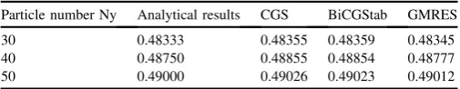
Table 4gives the comparison of different particle numbers in vertical direction Ny and accuracy comparisons of different iteration methods. According to the comparison ofTable 4, at the initial stage iteration there are some differences of the accuracy for different iteration methods. According to the comparisons of Table 4, GMRES method can get the highest accuracy among these three iteration methods.

In order to show the iteration steps of different iteration methods, Table 5gives the comparison of different iteration

Fig. 1. Calculation domain and its boundary conditions.

Fig. 2. Matrix elements distribution of ISPH_R (*¼non-zero element, blank space¼zero element, total particle number¼10*20).

Fig. 3. Pressure distribution by different iteration methods when tolerances errorRTOL¼10e6: a) Total pressure distribution Ny¼40; b) Comparison of different iteration methods whenx¼0.5 m.

Table 5

Comparison of iteration steps of different iteration methods and different preconditioner types Ny¼50.

Preconditioner type CGS (CPU time)

BiCGStab (CPU time)

GMRES (CPU time)

No precondtioner 163 (0.0223 s) 151 (0.0211 s) 107 (0.0194 s) Jacobi precondtioner 111 (0.0204s ) 101 (0.018 s) 87 (0.0172 s) ILU(0) preconditioner 56 (0.0189 s) 45 (0.0171 s) 32 (0.0162 s) Table 4

Comparison of different iteration methods by different particle numbers.

Particle number Ny Analytical results CGS BiCGStab GMRES

30 0.48333 0.48355 0.48359 0.48345

40 0.48750 0.48855 0.48854 0.48777

steps of different iteration methods and different precondi-tioner when Ny¼50. In order to show the convergence curve of iterative tolerance,Fig. 4 gives the comparison of conver-gence tests of different preconditioner for the GMRES as an example, andRTOL¼10e6. InFig. 4N_iter is the iteration step number and Err is the value ofrðnÞ_{inTable 3. According}

the results ofFig. 4, with the help of suitable preconditioner, GMRES can get fast convergence speed and less iteration steps. According to the results ofTable 5, GMRES method can get the least iteration steps. Furthermore, preconditioner is helpful for decreasing the iteration steps. According to the comparison of no preconditioner, Jacobi preconditioner and ILU(0) preconditioner, ILU(0) can get the least iteration steps. Although many different iteration methods can be set as the preconditioner, Jacobi and ILU(0) are the most popular and typical precondtioners. The comparisons of more complex preconditioner are not included at present, which can be done in further investigation.

According to the comparisons of CPU time in Table 5, ILU(0) can get the fastest convergence speed. As the calcu-lation process of ILU(0) is more difficult than Jacobi pre-conditioner, so the CPU time of ILU(0) preconditioner is a litter bit more than the ones of Jacobi compared with the a large decreasing of iteration steps. In order to show the effects of RTOL, Table 6 shows the accuracy of different RTOL by different iteration methods, and in this case the preconditioner is set as ILU(0). According to the comparison of different

RTOL, whenRTOL < 1.0e6, RTOLdoes not affect the ac-curacy of last results obviously. The rules are almost the same for these three iteration methods. So based on the series comparison of different iteration methods and different pre-conditioners, the preconditioner is set as ILU(0) and the

RTOL¼1.0e6 during the part of numerical tests.

6. Numerical tests and analysis

6.1. Dam breaking

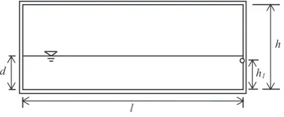
Dam breaking is often used as a benchmark for violent free surface flow. In this numerical test, a rectangular water column is confined by bottom, top wall and two vertical walls, as illustrated inFig. 5. The width of the water column island its

Fig. 4. Pressure distribution by different iteration methods when tolerances errorRTOL¼10e6.

Table 6

Comparison of calculation accuracy of different iteration methods with different tolerances when Ny¼50.

Tolerence (RTOL) Analytical results 1.0e5 1.0e6 1.0e10 1.0e15 CGS 0.49000 0.49031 0.49027 0.49026 0.49026 BiCGStab 0.49000 0.49028 0.49026 0.49025 0.49025 GMRES 0.49000 0.49013 0.49012 0.49012 0.49012

Fig. 5. The sketch of dam breaking model.

height ish. At the beginning of the computation, the dam is instantaneously removed and the water collapses and flows out along a dry horizontal bed. w is the distance between two vertical walls. There is one pressure sensors p1 on the right

vertical wall, the height of p1 from the bottom is h1. In this

section, all variables and parameters are non-dimensionalised usinghandg, such ast¼~tpffiffiffiffiffiffiffiffig=hunless mentioned otherwise. Although the case of non-breaking waves is not necessarily dealt with by the ISPH, it is used here for preliminary vali-dation of different iteration methods. In the first case,

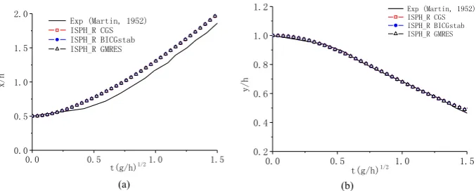
h¼1.0 m,l/h¼0.5,w/h¼4.5, the water collapses, just flows out along a dry horizontal bed, and stops before the wave front hits the right vertical wall. There are some experimental data for wave front and wave height on left vertical wall (Martin

and Moyce, 1952). Fig. 6 gives the comparison of wave fronts and wave heights obtained by three iteration methods using 100*200 particles. There is very little difference among three methods. The numerical results of the ISPH_R can get a good agreement with experimental ones by using the three iteration schemes. Although it can be found some difference on this case of wave front, it is as justified by other mesh based methods, which is shown in Zheng et al. (2014).

The pressure distribution and time histories are then examined. For the case withh¼1.0 m,l/h¼2.0,w/h¼5.366, there is a pressure sensor installed on the right vertical wall and with the height ofh1/h¼0.1833.Fig. 7gives the results of

dam breaking profiles and pressure distribution at different times. In this case the particle number is 20,000, time stepping

Fig. 7. Snapshot of wave profile and pressure distribution of dam breaking at different time.

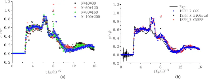
Fig. 9. Comparison of pressure time history of ISPH_R by different iteration methods: (a) Convergence test of different particle numbers by GMRES; (b) Comparison of CGS, Bi-CGstab, GMRES and experimental data, N¼100*200.

length d~t¼0:008, the iteration method is GMRES as example.Fig. 8gives the results of convergence tests on wave profiles according to different particle numbers. Fig. 9gives the comparison results of impact pressure at point p1 by

different iteration methods.Fig. 9 (a)is the convergence tests

of pressure time histories by different particle numbers by GMRES method. Fig. 9 (b) is the comparison of numerical results with experiment data (Colagrossi and Landrini, 2003) when particle number N ¼ 20,000. There is very little dif-ference between pressure time histories obtained by these three iteration methods. The results of pressure time histories have a good agreement with experimental data.

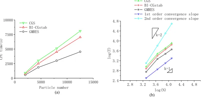
All codes run on the same computer, the CPU is Xeon E5-2665, 2.4 GHz, and the RAM is 16.0 GB.Fig. 10gives the comparison of CPU time corresponding to the particle numbers. In this figure, T is the CPU time and N is the particle number. When the particle number is small, e.g., 3200, the difference in the results from the three iteration methods is not very large. With the particle number increasing, such as 20,000, the CPU time of GMRES is 0.697 of that for the Bi-CGstab and 0.633 of that of the CGS. According to the results ofFig. 6(b), in the case of the dam breaking simulation, the convergent rate of three iteration methods is between the first order and second order.Table 7

gives the details of CPU time of three iteration methods. It can be seen that the GMRES can save more CPU time for the cases with more particles.

Fig. 10. Comparison of CPU time for dambreaking simulation by using different iteration methods: (a) CPU-time comparison, (b) Convergence-rate comparison.

Table 7

CPU time comparison for dam breaking simulation.

Particle number 40*80 60*120 80*160 100*200

CPU time(s) GMRES 305.8 709.4 1328.3 2082.2 Bi-CGstab 343.6 804.1 1602.2 2987.7 CGS 375.2 950.2 1910.2 3289.2

Fig. 11. Sketch of sloshing tank.

6.2. Violent water sloshing

In this section, violent sloshing flow will be considered. The geometry of this tank is rectangle withl¼0.6m,h¼0.5l,

d¼0.4h. The tank motion in sway displacement is given by

Xs¼a0ð1cosUtÞ, where a0 and U are the amplitude and

frequency of excited motion respectively. The parameters for this case are taken as a0 ¼0.05 m andT0 ¼2p=U¼1:5 s,

which are the same as those in Kishev et al. (2006) and is shown in Fig. 11. The behaviors of the ISPH_R method are further examined by modeling this case. For this purpose, different numbers of particles are employed withN ¼2000, 4500, 8000 and 12,500 respectively. Time step length is

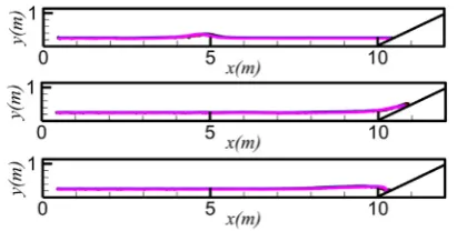
d~t¼0:008.Fig. 12gives the free surface profiles and pressure distribution at different time instants by GMRES when

N ¼8000.Fig. 13 gives the convergence test of free surface profile at different time by different particle numbers. Ac-cording to the comparison, the free surfaces for different number of particles are the almost same when breaking does not occur. However when breaking happens, there exists some differences between the profiles for different particle numbers.

Fig. 14 (a)gives the convergence test of pressure time histories for different particle numbers with the GMRES method at Point h1/l ¼ 0.1667 on the left wall. The pressure time

his-tories obtained by different particle numbers do not show significant differences, though there is some little difference near wave impact peaks.Fig. 14 (b)shows the comparison of pressure time histories of experimental data (Kishev et al., 2006) and numerical results obtained by CGS, BI-CGstab and GMRES respectively. It is noted that the experimental

Fig. 13. Convergence test of free surface profile by GMRES method for violent water sloshing:BN¼20*100, N¼30*150; N¼40*200; N¼50*250.

Fig. 14. Comparison of pressure time history of ISPH_R by different iteration methods for violent sloshing simulation: (a) Convergence test of pressure time history by different particle numbers with GMRES method; (b) Comparison of pressure time history of CGS, Bi-CGstab, GMRES and experimental data, N¼50*250.

pressure time history given in Kishev et al. (2006) did not show the transient period that must exist and they did not mention whether it was recorded on the left or on right walls. To compare our results with their experimental data, the time for the experimental results in the figure has been adjusted so that the 3rd pressure peak of the numerical results corresponds to the first peak in their paper. These figures show that the results from all the methods have similar patterns to the experimental one and that the time intervals between two consecutive impacts are almost the same.

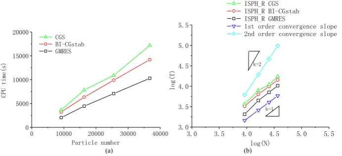
The computer used for running these cases is the same as in the previous section. Fig. 15 gives the comparison of CPU time corresponding to the different particle numbers. In the numerical tests, the CPU time of GMRES is still less than that of CGS and Bi-CGStab, and the GMRES saves more time for the cases with large particle numbers again. The convergence rates of three methods are almost the same, but the values of the GMRE are always below the ones of CGS and Bi-CGstab.

Table 8 gives the details of CPU time of three iteration methods for this case.

6.3. Solitary wave slamming

This section considers the test of solitary wave slamming. The interaction between solitary wave and structures are the topic related to many coastal and ocean engineering. The solitary wave is often used to represent certain characteristics of the incident wave. In this section, the ISPH_R method is applied to the simulation of the solitary wave impact on walls with a fixed angle. The numerical results will be compared with the experimental data. Furthermore, the results of different iterative schemes are also given for CPU efficiency and precision behavior comparison.

Fig. 16shows the geometry and setup of simulation on the cases in the section. On the left end it has a piston wave maker and on the other end it has a slope beach. In order to make a solitary wave by a piston wave maker, the analytical solution for the wave profile can be derived from the Boussinesq equation, the displacement of piston of different time is shown as

xpðtÞ ¼

ffiffiffiffiffi

4a

3d r

d h

tanhn ffiffiffiffiffiffiffiffiffiffiffiffiffiffip3a=4d3½_ct_xðtÞ l o

þtanh

lpffiffiffiffiffiffiffiffiffiffiffiffiffiffi3a=4d3 i

ð24Þ

where xp is piston displacement,a is wave amplitude,d is

water depth andc¼pffiffiffiffiffiffiffiffiffiffiffiffiffiffiffiffiffigðdþaÞis the solitary wave celerity,tis the non-dimensional time. It should adopt the iterative method to get the value ofxp. In this case,his the height of whole slope and

h¼1.0 m, wave amplitudea/h¼0.15, water depthd/h¼0.25, the total tank length isl/h¼10.0, slope anglea¼150. In the area of slope beach, a local coordination transformation is used

Table 8

CPU time comparison for violent water sloshing calculation.

Particle number 20*100 30*150 40*200 50*250

CPU time(s) GMRES 564.3 1853.7 3006.2 4534.5 Bi-CGstab 760.2 2511.3 4504.9 7030.6 CGS 910.6 3010.3 5101.2 8103.3

Fig. 16. The model of wave tank for solitary wave slamming.

Fig. 17. Snapshots of profile and pressure distribution for solitary wave slamming of different time: (a)et¼0.0; (b)et¼10.5; (c)et¼18; (d)et¼20.4;

(e)et¼22.5; (f)et¼24.0

for the solid wall handling of a certain angle.Fig. 17depicts the results of wave profile and pressure distribution at different time. The iteration method uses GMRES method as example and particle number for this case is 36,760, and the time step is

d~t¼0:008.Fig. 18gives the convergence test of wave elevation by different particle numbers and the iteration method is GMRES. There is a pressure sensor fixed on the slope, the height

h1is the vertical distance from bottom andh1/h¼0.05. The same

scale experiment are carried on HEU (Zheng et al., 2015).Fig. 19

gives the comparison of pressure time history atp1between

nu-merical and experimental results by three iteration methods. The

results of the ISPH_R have a quite good agreement with exper-imental ones. There still exist some oscillations in time history for ~

t¼22:5 in experimental data, similar behaviors are observed in the results from three iteration methods. Fig. 20 depicts the comparison of CPU time for solitary wave slamming simulation by different iteration methods. The conclusion is very similar to that in previous section, i.e., the GMRES saves more time for the cases with large particle numbers and the convergence rates of both method are almost the same. More details of CPU time for different iterative methods is shown inTable 9.

7. Conclusions

This paper presents a comparative study of different itera-tion methods for solving pressure Poisson equaitera-tion for incompressible SPH based on Rankine source solution. Three iteration methods includes CGS, BI-CGstab and GMRES. The different CPU time and convergence rates are examined. The numerical test cases include still water test, dam breaking,

Fig. 19. Comparison of pressure time history of ISPH_R by different iteration methods for solitary wave slamming.

Fig. 20. Comparison of CPU time for solitary wave slamming by different iteration methods: (a) CPU-time comparison; (b) Convergence-rate comparison.

Table 9

CPU time comparison for solitary wave slamming calculation.

Particle number 9185 16333 25525 36760

violent water sloshing and solitary wave slamming, which are the typical applications for ocean engineering. The numerical results are compared with experimental data. From the nu-merical test results and comparisons, we come to the following conclusions:

(a) With the help of one of these three linear equation solvers, incompressible SPH based on Rankine source solution can give smoothed and reliable pressure distribution.

(b) All iteration methods, CGS, BI-CGstab and GMRES have the convergence rate of between first order and second order. The preconditioner is import for different iteration methods, suitable preconditioner can decrease the iteration steps obviously. Furthermore, the tolerance of different iteration schemes can affect the accuracy of last results, but whenRTOL is small enough (like RTOL <1.0e6), the iteration results may not get very improvement significantly. From the comparison of different iteration schemes, the CPU time spent by GMRES is about 0.7e0.6 time of that by Bi-CGstab and CGS.

The above conclusions are based on the series code but the study on the iteration methods in parallel calculation for ISPH_R method is still ongoing.

Acknowledgement

This work is sponsored by The National Natural Science Funds of China (51009034, 51279041, 51379051, 51579054, 51639004), Foundational Research Funds for the central Universities (HEUCDZ1202, HEUCF120113) and Defense Pre Research Funds program (9140A14020712CB01158), to which the authors are most grateful. The second author also wishes to thank the Chang Jiang Visiting Chair professorship of Chinese Ministry of Education, hosted by the HEU.

References

Bonet, J., Lok, T.S., 1999. Variational and momentum preservation aspects of smooth particle hydrodynamics formulation. Comput. Methods Appl. Mech. Eng. 180, 97e115.

Colagrossi, A., Landrini, M., 2003. Numerical simulation of interfacial flows by smoothed particle hydrodynamics. J. Comput. Phys. 191, 448e475. Cummins, S.J., Rudman, M., 1999. An SPH projection method. J. Comput.

Phys. 152, 584e607.

Ellero, M., Serrano, M., Espanol, P., 2007. Incompressible smoothed particle hydrodynamics. J. Comput. Phys. 226, 1731e1752.

Ferrand, M., Laurence, D.R., Rogers, B.D., Violeau, D., Kassiotis, C., 2013. Unified semi-analytical wall boundary conditions for inviscid, laminar or turbulent flows in the meshless SPH method. Int. J. Numer. Meth. Fluids 71, 446e472.

Fujino, S., 2002. GPBICG (m, l): a hybrid of BiCGSTAB and GPBiCG methods with efficiency and robustness. Appl. Numer. Math. 41, 107e117.

Hori, C., Gotoh, H., Ikari, H., Khayyer, A., 2011. GPU-acceleration for moving particle semi-implicit method. Comput. Fluids 51, 174e183. Hu, X.Y., Adams, N.A., 2007. An incompressible multi-phase SPH method.

J. Comput. Phys. 227 (2), 264e278.

Khayyer, A., Gotoh, H., 2011. Enhancement of stability and accuracy of the moving particle semi-implicit method. J. Comput. Phys. 230, 3093e3118.

Khayyer, A., Gotoh, H., Shao, S.D., 2008. Corrected incompressible SPH method for accurate water-surface tracking in breaking waves. Coast. Eng. 55 (3), 26e50. Kishev, Z.R., Hu, C.H., Kashiwagi, M., 2006. Numerical simulation of violent

sloshing by a CIP-based method. J. Mar. Sci. Technol. 11, 111e122. Koshizuka, S., Oka, Y., 1996. Moving particle semi-implicit method for

fragmentation of incompressible fluid. Nucl. Sci. Eng. 123 (3), 421e434. Koshizuka, S., Ikeda, H., Oka, Y., 1999. Numerical analysis of fragmentation mechanisms in vapour explosions. Nucl. Eng. Des. 189 (1e3), 423e433. Lee, E.S., Moulinec, C., Xu, R., Violeau, D., Laurence, D., Stansby, P., 2008. Comparisons of weakly compressible and truly incompressible algorithms for the SPH mesh free particle method. J. Comput. Phys. 227, 8417e8436.

Liu, X., Xu, H.H., Shao, S.D., Lin, P.Z., 2013. An improved incompressible SPH model for simulation of wave - structure interaction. Comput. Fluids 71, 113e123.

Lind, S.J., Xu, R., Stansby, P.K., Rogers, B.D., 2012. Incompressible smoothed particle hydrodynamics for free-surface flows: a generalised diffusion-based algorithm for stability and validations for impulsive flows and propagating waves. J. Comput. Phys. 231, 1499e1523.

Liu, M.B., Liu, G.R., 2006. Restoring particle consistency in smoothed par-ticle hydrodynamics. Appl. Numer. Math. 56, 19e36.

Ma, Q.W., Zhou, J., 2009. MLPG_R method for numerical simulation of 2D breaking waves. Comput. Model. Eng. Sci. 43 (3), 277e304.

Martin, J.C., Moyce, W.J., 1952. Part IV: an experimental study of the collapse of liquid columns on a rigid horizontal plane. Phil. Trans. R. Soc. Lond. A 244 (882), 312e324.

Mittal, R.C., Alaurdi, A.H., 2003. An efficient method for constructing an ILU preconditioner for solving large sparse nonsymmetric linear systems by the GMRES method. Comput. Math. Appl. 45, 1757e1772.

Monaghan, J.J., 1994. Simulation free surface flows with SPH. J. Compu. Phys. 110 (4), 399e406.

Oger, G., Doring, M., Alessandrini, B., Ferrant, P., 2007. An improved SPH method: towards higher order convergence. J. Comput. Phys. 225, 1472e1492. Rafiee, A.R., Cummins, S., Rudman, M., Thiagarajan, K., 2012. Comparative study on the accuracy and stability of SPH schemes in simulating energetic free-surface flows. Eur. J. Mech. B/Fluids 36, 1e16.

Saad, Y., 2003. Iterative Methods for Sparse Linear Systems (Second Version). Society for Industrial and Applied Mathematic.

Saad, Y., Schultz, M.H., 1986. GMRES: a generalized minimum residual al-gorithm for solving nonsymmetric linear systems. SIAM J. Sci. Stat. Comput. 7, 856e869.

Schwaiger, H.F., 2008. An implicit corrected SPH formulation for thermal diffusion with linear free surface boundary conditions. Int. J. Numer. Meth. Engng. 75, 647e671.

Shadloo, M.S., Zainali, A., Yildiz, M., Suleman, A., 2012. A robust weakly compressible SPH method and its comparison with an incompressible SPH. Int. J. Numer. Methods Eng. 89 (8), 939e956.

Shao, S.D., 2009. Incompressible SPH simulation of water entry of a free-falling object. Int. J. Numer. Meth. Fluids 59 (1), 91e115.

Shao, S.D., Lo Edmond, Y.M., 2003. Incompressible SPH method for simu-lating Newtonian and non-Newtonian flows with a free surface. Adv. Water Resour. 26 (7), 787e800.

Shao, S.D., Ji, C.M., Graham, D.I., Reeve, D.E., James, P.W., Chadwick, A.J., 2006. Simulation of wave overtopping by an incompressible SPH model. Coast. Eng. 53 (9), 723e735.

Sleijpen, G.L., Fokkema, D.R., 1993. BiCGstab(L) for linear equations involving unsymmetric matrices with complex spectrum. Electron. Trans. Numer. Analysis 1, 11e32.

Sonneveld, P., 1989. CGS, A fast Lanczos-type solver for nonsymetric linear systems. SIAM J. Sci. Stat. Comput. 10, 36e52.

Spyropoulos, A.N., Palyvos, J.A., Boudouvis, A.G., 2004. Bifurcation detec-tion with the (un) precondidetec-tioned GMRES(m). Comput. Methods Appl. Mech. Eng. 193, 4707e4716.

Vogel, J.A., 2007. Flexible BiCG and flexible Bi-CGSTAB for nonsymmetric linear systems. Appl. Math. Comput. 188, 226e233.

Van der Vorst, H.A., 1992. Bi-CGSTAB: a fast and smoothly converging variant of Bi-CG for solution of non-symmetric linear system. SIAM J. Sci. Stat. Comput. 13, 631e644.

Xu, R., Stansby, P., Laurence, D., 2009. Accuracy and stability in incom-pressible SPH (ISPH) based on the projection method and a new approach. J. Comput. Phys. 228 (18), 6703e6725.

Zhang, S., Morita, K., Kenji, F., Shirakawa, N., 2006. An improved mps method for numerical simulations of convective heat transfer problems. Int. J. Numer. Methods Fluids 51, 31e47.

Zheng, X., Ma, Q.W., Duan, W.Y., 2014. Incompressible SPH method based on Rankine source solution for violent water wave simulation. J. Comput. Phys. 276, 291e314.