Nephroblastoma analysis in MRI images

NEPHROBLASTOMA ANALYSIS IN MRI IMAGES

Djibril Kaba

_{, Nigel McFarlane}

_{, Feng Dong}

_{, Norbert Graf}

_{and Xujiong Ye}

e-mail: djibkaba@hotmail.com, nigel.mcfarlane@beds.ac.uk, feng.dong@beds.ac.uk, norbert.graf@uniklinikum-saarland.de, jni@lincoln.ac.uk

(Received August 12, 2018; revised June 3, 2019; accepted June 11, 2019)

NEPHROBLASTOMA ANALYSIS IN MRI IMAGES

D

K

N

M

F

F

D

N

G

X

Y

1_{Department of Computer Science and Technology, University of Bedfordshire, University Square, Luton LU1} 3JU, UK,2_{Department for pediatric hematology and oncology at Saarland University Hospital, Building 9} 66421 Homburg, Germany,3_{School of Computer Science, University of Lincoln, Brayford Pool Lincoln} Lincolnshire LN6 7TS, UK

e-mail: djibkaba@hotmail.com (Submitted)

ABSTRACT

The annotation of the tumour from medical scans is a crucial step in nephroblastoma treatment. Therefore, an accurate and reliable segmentation method is needed to facilitate the evaluation and the treatments of the tumour. The proposed method serves this purpose by performing the segmentation of nephroblastoma in MRI scans. The segmentation is performed by adapting and a 2D free hand drawing tool to select a region of interest in the scan slices. Results from 24 patients show a mean root-mean-square error of0.0481_±0.0309, an average Dice coefficient of 0.9060_±0.0549 and an average accuracy of 99.59%_±0.0039. Thus the proposed method demonstrated an effective agreement with manual annotations.

Keywords: Continuous Max-Flow, Graph Segmentation, Kernel Induced Space, MRI images, Nephroblastoma, Wilms tumour.

INTRODUCTION

Nephroblastoma or Wilms’ tumour is a form of kidney cancer that affects around 80-85 children in the UK each year (Macmillan Cancer Support, 2016). Nephroblastoma generally affects children below the age of five and it may begin to develop in the womb when the baby is still unborn. The most common symptom is a painless swelling in the abdomen. Nephroblastoma rarely affects adults. In most cases it affects only one kidney (unilateral), but it can also affect both (bilateral). Nephroblastoma is a fast growing tumour with a median tumour size of around 400 ml at the time of diagnosis. Fortunately due to prospective clinical trials and effective treatments more than 90% of patients can be cured today. Imaging analysis tools play an important role in diagnosis and treatment planning. The assessment of the tumour during preoperative chemotherapy is of prognostic relevance and is crucial for postoperative treatment stratification (David et al., 2012).

Over the past years, many segmentation methods of different types of tumours such as glioblastoma, prostate and Wilms) have been proposed (Baueret al., 2013a; Gordilloet al., 2013; Phamet al., 2000). These methods include full automated and semi-automated methods and they are applied to interpret scans such as MRI, CT or ultrasound. Each technique has its own advantages and disadvantages. Many of these methods fail due to different acquisition conditions

of resolution, illumination and field of view, and the variability of body shapes and positions.

Overlapping tissue and organs and the irregular size of the tumours can also cause a significant degradation to the performance of the segmentation methods, particularly the fully-automated methods. For the above reasons, there is a need for reliable and robust semi-automated segmentation methods for Wilms’ tumour studies. Semi-automated tumour segmentation techniques are computational methods that perform an extraction of the tumour tissue from multi-sequence Magnetic Resonance Imaging (MRI) with the interaction of human experts. These methods can provide important time-saving for neuro-radiologists in tumour assessment, and their accuracy can enhance tumour characterisation for radiotherapy, surgical planning and drug development assessment. The aim of this document is to report findings during the CHIC project for semi-automated Nephroblastoma tumour segmentation in multi-sequence MRI imaging. In the following section, we briefly review some previously-proposed tumour segmentation methods.

RELATED WORKS

Advance innovation in hardware and software is leading to a continuing increase in computing power. This has made supervised classification techniques an attractive research area (Menze et al., 2015) in the medical image analysis. The performance of these methods relies heavily on a large set of training data, which include manually annotated images for learning features in the medical scans. Neural Networks (Goceri and Goceri, 2015; Ramrez et al., 2018; Zhong et al., 2018), Support Vectors Machines (Lee et al., 2008; Amiriet al., 2016) and Random Forests (Shah et al., 2017; Bauer et al., 2012; Conze et al., 2016) are amount the popular methods used for medical images segmentation. Unlike these supervised methods, unsupervised segmentation techniques are very flexible as they can be applied on a small set of data from which they can learn classification rules based some similarity criterion.

The segmentation of Wilms tumour is not a trivial task due the complexity, inhomogeneity and variability of its structures Farmakiet al.(2010) and may require inputs such as seed-points, location and shapes from human experts. For this reason, a fully automated segmentation method may not be a good option for clinical use (Farmakiet al., 2010; Davidet al., 2012). Thus, a semi-automatic tumour segmentation method can be a good alternative option for Wilms’ tumour analysis in multi-sequence MRI scans.

The semi-automated tumour segmentation methods can be divided into three major groups (Farmaki et al., 2010): region-based approaches, deformable model-based approaches and graph-based approaches. The region-based approaches perform the tumour segmentation using a single seed point and expand the pixel extraction from that seed point to fill a defined coherent region according to a similarity measure of neighbouring pixels within the image region (Adams and Bischof, 1994). The region-based approaches include region-growing and watershed methods. A typical region-growing approach was proposed in (Kim and Park, 2004) by Kim and Park. This combined the region-growing algorithm with a texture-based analysis operation, which was performed on sample images of the tumour to define a seed region as a starting point of the region-growing algorithm. Mancas (Mancas and Gosselin, 2003) proposed a semi-automatic segmentation on head and neck tumours in CT, MRI and PET scans. The approach used a marker-based watershed technique, by incorporating a fuzzy region with a tumour probability from 0 to 1. The watershed algorithm was used iteratively. This combination improved the watershed algorithm and avoided the over-segmentation problem. In (Sauwenet al., 2016),

Nicolas et al., presented a semi-automated framework for segmenting brain tumour from multi-sequence MRI scans using regularisation non-negative matrix factorisation. The technique makes use of the tumour regions seeds selected by the user to initialise the algorithm. A morphological post-processing technique is used to improve the segmentation results, which combined the special location voxels with some adjacency constraints defined in the process.

The region-based methods have specific advantages over other segmentation approaches: they are easy to implement and produce coherent regions. However they often perform poorly because they cannot find objects that span several disconnected areas, and decisions regarding region membership can be difficult. Methods presented in (Kim and Park, 2004), (Mancas and Gosselin, 2003), and (Sauwen et al., 2016), relied heavily on the selection of the seeds in the pathology region (i.e., tumours voxels) as a starting point to initialise the algorithm. The intensity variation in the tumour region can led to a misclassification of tumour pixels. Our method addresses this issue by interactively selecting a wider region of the tumour area which include different variation of the tumours voxels intensity.

segmentation technique based on level set deformable algorithm. The method uses both the images gradient information and the reginal data information to deform the level set algorithm. They estimated the velocity forces based the tumour voxels statistical measure and surrounding health tissues information. The above deformable segmentation methods can perform well on medical images. However, their implementations can be very complex and costly. Any sharp intensity variation, artefacts or noises in the medical images can led to misclassification. Our method avoids these issues using a bias correction operation as a pre-processing step to remove all the imaging artefacts, noise and corrected the intensity inhomogeneity in the scans. In addition, the bias correction, we applied an energy function which includes both boundary and regional terms allowing the segmentation of heterogeneous objects, which not possible with deformable segmentation methods due to local minima. Furthermore, deformable model-based methods (Kainm¨uller et al., 2007; Liu et al., 2010; Zhan and Shen, 2006) use prior knowledge of the scan (i.e. intensities, shapes, colour, texture, positions etc.) to apply constraints on the segmentation algorithms. These constraints can lead to segmentation errors when the algorithms are used on different image modalities (Kaba et al., 2015). Our segmentation method addresses these issues by using a prior knowledge including intensities variation of the tumour, which is manually selected by the user.

The graph-based approach is one of the most attractive segmentation methods in Computer-aided diagnosis (CAD). Like the deformable model-based approaches, the graph-based image segmentations are also based on energy optimisation. They combine boundary regularisation with regularisation of regional proprieties in the same approach as Mumford-Shah (Boykov and Funka-Lea, 2006). The segmentation is performed by dividing the image into sub-classes known as Foreground (targeted tumour) and Background. The segmentation process is performed using a graph, which consists of a set of nodes (i.e. pixels) and a set of edges (i.e. weights on the nodes) that connect the nodes using their degrees of similarity (intensity) (Kabaet al., 2015).

In (Freedman and Zhang, 2005), Daniel Freedman and Tao Zhang presented an interactive graph cut algorithm, which incorporates shape priors into the energy function. The segmentation is performed by the shapes template and integrating the shape information in the weights on the edges in the graph. Xinjian Chen et al., (Chenet al., 2012) proposed a segmentation of method for abdominal 3-D organ. The segmentation is performed by combining the active appearance model,

live wire, and graph cuts. The overall method included model building, object recognition, and delineation. In (van der Lijn et al., 2008) Fedde van der Lijn et al., presented a graph cut segmentation algorithm for the extraction of the hippocampus from MRI scan. The graph energy functional contains the intensity energy and the prior energy which included a spatial and a regularity term. A 3D semi-automated graph cut-based segmentation algorithm of liver cancer is proposed in (Esneault et al., 2007). The liver cancer in a contrast-enhanced 3D CT volume was segmented with a user interaction in the selection of initial seeds for the foreground or background. These seeds are then used as a training base for the final segmentation of cancer tissue. Wei Ju et al., presented in (Ju et al., 2015) a lung tumour segmentation technique on PET-CT scans combining random walk with a graph cut algorithm. The random walk is used to initialise seeds for the graph cut algorithm and shape penalty cost is combined into the graph energy function to constrain the tumour area during segmentation. The graph-based segmentation methods are very powerful techniques because they allow the incorporation of prior knowledge (shapes, positions, sizes, seeds, textures) into the graph energy formulation to guide the algorithm defining the optimal segmentation results (Salazar-Gonzalez et al., 2014). The performance of graph-based techniques above depend highly on the selection of initial seed points (Esneault et al., 2007; Chen et al., 2012), shape constraints (Ju et al., 2015; Freedman and Zhang, 2005) and intensity variation in the images (Kaba et al., 2015; van der Lijnet al., 2008). As results they required parameters turning to be applied in different images data. We have addressed these problems, by incorporating a bias correction operation to correct corrected the intensity inhomogeneity and a graph cut algorithm, which allows the interaction of human expert to guide the algorithm.

The rest of the paper is organized as follows. Our segmentation method is discussed in Section 3. Section 4 highlights information about the data-set used in the study. Section 5 shows the experimental results of the proposed method and the conclusion is drawn in Section 6.

METHOD

choice for the analysis of nephroblastoma scans in the clinical domain. This allows the interaction of expert physicians in order to guide the segmentation algorithm.

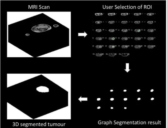
Our method serves this purpose, it allows the radiologists to interact with a 2D image slice. The first step of the segmentation algorithm consists of removing some common artefacts of MRI medical imaging from the scans (i.e. noise, intensity inhomogeneity). This pre-processing operation is performed using a bias correction algorithm (Tustison et al., 2010). The tumour extraction in multi-sequence MRI scans is performed by adapting a continuous max-flow min-cut approach (Yuanet al., 2010). This includes a free 2D hand drawing tool, which allows human experts to select a region of interest (i.e. tumour seeds) and a kernel-induced segmentation functional (Salah et al., 2011; 2014). The proposed method could provide time and cost saving in nephroblastoma annotation and it can be used for high-throughput studies, such as clinical trials. It will be incorporated in the segmentation tools for the Computational Horizons in Cancer (CHIC) project Stamatakos and Graf (2017), funded under the European Commission FP7 programme. Fig. 1 shows the illustration of the proposed method.

PRE-PROCESSING

Generally, the fuzziness of tumour boundary (lack of clear edges) in multi-sequence MRI scans is caused by the presence of imaging artefacts such as noise, inhomogeneity and similarity to surrounding tissues. The bias correction operation (Tustison et al., 2010) is used to correct these issues in the images to allow a correct segmentation of the tumour in the scan. The operation is performed by estimating the residual bias field. This residual is then subtracted from the corrupted scans to enhance the tumour. The bias correction operation can also reduce false positives during the segmentation pro

TUMOUR EXTRACTION

To perform the segmentation of nephroblastoma tumour from MRI scans, we represent each pixel point in a scan as a graph G(n,e), consisting of a set nodes n (i.e. pixels) and a set of edges e connecting neighbouring nodes or pixels{p,q_}Boykov and Jolly

(2001). The nodes also include two special nodes known as terminals S (foreground:tumour seeds) and T (background seeds). Each pair of neighbouring pixels

{p,q_} in the image grid is connected by n-links (i.e.

edge between pixels). Each pixel pin the scan is also

connected to the foreground terminal through the s-links with{p,s_}and to the background terminal with

t-links with{p,t_}.

The edges in the graph including both n-links and t-links are assigned some positive weights We > 0 based on the similarity measured between pixels (i.e. intensities). After creating the graph, the segmentation is performed by producing a cut through the graph. The preferred cut or path will have the minimum total weights of edges for travelling from a start node to an end node. The selected cut separates the MRI scan into two disjoint regions, one representing the tumour tissue (foreground) and the other one the rest of the image (background) as shown in Figure 3 2.

Ifs−t is the cut that separates the tumour tissue

(Fgor foreground pixels) from the rest of the image (Bg or background pixels), thens−trepresents a subset of edgesC2e where

|C|=

Â

e2C

We (1)

To formulate the energy function of the graph, letAbe an indexing function, whose components assign each pixel in the MRI image to a regionRl ={p2W|pis labelledl}:

A:p2W−!Ap2h (2)

where h is a finite set of binary labels (i.e., l =1

if Ip is a foreground pixel (Fg) and l =0 if Ip is a background pixel). Therefore, each label l in the MRI image grid represents either the tumour pixelFg (foreground) or the background pixel Bg dividing the image in two regions. From this the energy function of the segmentation can be defined as:

E(A) =B(A) + l_·R(A). (3)

whereB(A)represents the boundary term, it describes

the coherence between neighborhood pixels (base on their intensities). R(A) is the data term or regional

Fig. 1: Illustration of different processes of the proposed method. Top left: 3D MRI Image. Top right: 2D slice for user selection of ROI. Bottom left right: segmentation results of 2D slice. Bottom right: segmentation result in 3D.

B(A) =

Â

f(Ap,Aq) (4)

where

f(Ap,Aq) =1 forAp6=Aq

f(Ap,Aq) =0 otherwise

(5)

Bp,q=exp(−(Ip−Iq) 2

2s2 )· 1

d(p,q) (6)

where Bp,q evaluates the discontinuity between neighbouring pixels in W. The value of Bp,q is large when the pixels intensitiesIpandIq are similar and it is close to zero otherwise Boykov and Jolly (2001).s

is the standard deviation and d is the distance between two pixels (p and q) Boykov and Jolly (2001). The values of both parameters were defined experimentally wheres=5e−4andd=0.11 Similarly the data term is

defined as:

R(A) =

Â

Rp(Ap) =

Â

Â

−logP(Ip|Rl). (7)

whereRlrepresents the scan region that has labelland P(Ip|Rl)is the conditional probability that measures the likelihood of a pixel intensity(Ip)in the scan grid given a model distribution in each image region Rl. Due to the complexity of the MRI scan, the piecewise Gaussian distribution, which is often used as piecewise constant segmentation model is not always sufficient to extract the tumour tissue from a nonlinearly separable MRI image. For this reason, the data term of the graph

formulation is implicitly transformed by mapping the original MRI data into a higher dimensional feature space using a kernel function (Salah et al., 2011; 2014), where the piecewise constant model of the graph cut formulation is applicable. This process allows a linear separation in the image data.

Letkl be the piecewise constant model parameter of an image region Rl, then the data term (7) can be defined as:

R(A) =

Â

Rp(Ap) =

Â

Â

(k_l−I_p)2. (8)

Ify(.)is a nonlinear mapping function from the MRI

data spaceQto a higher dimensional feature spaceD. The graph cut formulation becomes:

E(_{k_l},A) =

Â

Bp,q·f(Ap,Aq)

+l·

Â

Â

(y(kl)−y(Ip))2. (9)

After assigning a unique label to each pixel, the MRI image can be divided into two regions with each region containing one label. In this case a kernel induced space image segmentation with the graph cut would simply result in finding the labelling which minimises the graph formulation (9). By applying Mercer’s theorem and simplifying Salahet al.(2011),

(y(k_l)₋y(I_p))2 in (9), we obtain the following

E({kl},A) =

Â

Bp,q·f(Ap,Aq)

+l_·

Â

Â

R(I_p,k_l). (10)

The expression in (10) depends on both the labelling function A, the image region parameter kl and it is optimised using max-flow algorithm Yuan et al. (2010). This optimisation process allows a separation of the tumour tissue from the MRI scan.

The interactive segmentation is performed as follows: The slices in a scan are displayed as a single image object as shown in Fig. 2. This operation allows the user to visualize all the slices that contain the tumour. The expert user can select tumour seeds region in one of the tumour slices (red circle in Fig. 2). The intentisty values of the selected tumour seeds is used as the foreground seeds of the gragh. Then the likelihood of each pixel p in the scan belonging to the tumour pixels is meseaued using (10).

The rest of the slices are automatically segmented in the scan by the proposed method as shown in (Fig. 2 (b)). One of the advantages of this interactive segmentation is that it allows radiologists to interactively select tumour seeds in one of the scan slices to allow a complete extraction of the tumour and avoid the segmentation of health tissues or other tissues similar to the tumour. It is also allows a global optimal solution for a graph segmentation, which is not possible in a fully automated segmentation methods.

DATA SET

The multi-sequence MRI scan data used in this study was obtained from ongoing pioneering research conducted on Wilms tumour in the department of Paediatric Oncology and Haematology at Saarland University Medical Centre in Homburg, Germany. The data set contains a sequence of T2 weighted multi-sequence MRI scans with transversal cut of 24 cancer patients. The acquisition parameters of multi-sequence MRI are set differently by the operators to allow a better visualisation of different scans as seen a Table 1.

Table 1: Details information of the dataset use in the study. P = Patient, R.T = Repetition Time, E.T = Echo Time, I.S = Inslice Sampling, S.T = Slice Thickness, S.S = Spacing between Slices.

P R.T E.T I.S S.T S.S

Fig. 2: User Selection of ROI. (a) the user expertise is needed to select a tumour tissue (red circle) in one of the 3D image slices, the rest of the tumour tissues are segmented automatically by the proposed algorithm. (b) the segmentation results of the method. (c) manually labelled image slices.

predominant, mixed histology or regressive) and high risk tumour (blastemal predominant). In total we have 48 scans from the 24 patients including before and after chemotherapy. The tumour area of each scan was manually annotated by an experienced radiologist with a total hand labelled of 48 images. These expert hand labelled images were used as benchmark (ground truth) to evaluate the performance of our segmentation method. This study has not measured the inter and intra observer variability due to the unavailability of additional hand labelled data-set.

RESULTS AND DISCUSSIONS

The proposed method is implemented on MATLAB R2011b and the computation time of our algorithm is less than 80 seconds for each multi-sequence MRI scan on a MAC OX X running at 2.66 GHz, with 4G of RAM memory. To evaluate the accuracy of our method, we compared our results against the experts manual annotations. The evaluation is performed using statistical metrics such as the sensitivity (true positive rate), the specificity (true negative rate), the false negative rate and the average accuracy rate are shown in Table 2. Others metrics including the Dice coefficient, the root-mean-error and the Jaccard index are also used for the validation of spatial tumour shape representation in Table 3.

Table 2 shows the evaluation results of the proposed method using the above metrics on all the 48 scans. The proposed method achieves a high performance with average accuracy of 99.59%, TPR=94.52% and

FPR=0.34%. The same performance is also observed

in Table 3 with a Dice coefficient of 0.9060, Jaccard

index of 0.8326 and an average RMSE of 0.0481.

An overview of the performance results shows that the proposed method achieved a good agreement with experts manual labelled tumour boundaries.

To facilitate the performance comparison between our method and the experts hand-labelled tumours, we

also tested our method separately on scans before and after radio-chemotherapy. Table 4 and Table 5 compare the performance of the proposed method on the scans before and after treatment. An overview of the results shows that in both scans, our proposed method is in good agreement with experts manual labelled. However the segmentation of the scans after radio-chemotherapy performs slightly better than the one before radio-chemotherapy: around 0.18% better

on average accuracy. In addition to the tables, Fig.3 shows the box plots of Dice coefficient, RMSE, TNR and TPR of the all scans. Fig.4 shows the segmentation results comparison of the proposed method against the experts hand-labelled tumour. Fig.5 shows the segmentation results of a scan before and after the radio-chemotherapy.

For additional illustration, we performed the box plots of the Dice coefficient, RMSE, TNR and TPR for the evaluation of our method as shown in Fig 3.

Fig.6 illustrates the importance of the semi-automated segmentation method for Wilms’ tumour. In Fig.6 (a) without the expert knowledge, it is almost impossible to define the tumour region due the non-uniformity of the scan intensity and the irregular shape of the tumour. Therefore the need of expert input (i.e. selection of tumour seeds) is essential for the extraction of the tumour from the scan. This shows the importance of semi-automatic segmentation methods in Wilms’ tumour segmentation, which is not possible in fully automated segmentation methods.

Metrics Average Std Conf

Sensitivity (TPR) 0.9452 0.0429 0.0077 Specificity (TNR) 0.9966 0.0039 0.0007 FPR 0.0034 0.0039 0.0007 FNR 0.0548 0.0429 0.0077 ACC 0.9959 0.0039 0.0007

Table 3: Performance evaluation of the tumour tissue segmentation using the Dice coefficient, the root-mean-square (RMSE) and the Jaccard index with their respective standard deviation and 95% confidence interval (Conf). - 48 scans

Metrics Average Std Conf

Dice 0.9060 0.0549 0.0098 Jaccard 0.8326 0. 0898 0.0161 RMSE 0.0481 0.0309 0.0055

Table 4: Performance evaluation of the tumour tissue segmentation using true positive rate (TNR), false positive rate (FNR) and the accuracy ACC) with their respective standard deviation (Std) and 95% confidence interval (Conf). - 24 scans before and after radio-chemotherapy

Before therapy Average Std Conf

Sensitivity (TPR) 0.9446 0.0355 0.0064 Specificity (TNR) 0.9960 0.0044 0.0008 FPR 0.0040 0.0044 0.0008 FNR 0.0554 0.0355 0.0064 ACC 0.9950 0.0042 0.0008

After therapy Average Std Conf

Sensitivity (TPR) 0.9458 0.0500 0.0089 Specificity (TNR) 0.9972 0.0033 0.0006 FPR 0.0028 0.0033 0.0006 FNR 0.0542 0.0500 0.0089 ACC 0.9968 0.0034 0.0006

Table 5: Performance evaluation of the tumour tissue segmentation using the Dice coefficient, the root-mean-square (RMSE) and the Jaccard index with their respective standard deviation (Std) and 95% Confidence Interval (Conf). - 24 scans before and after radio-chemotherapy

Before therapy Average Std Conf

Dice 0.9046 0.0425 0.0076 Jaccard 0.8285 0.0705 0.0126 RMSE 0.0551 0.0290 0.0052

After therapy Average Std Conf

Dice 0.9074 0.0660 0.0118 Jaccard 0.8367 0.1070 0.0191 RMSE 0.0411 0.0317 0.0057

Fig. 3: Box plots of Dice coefficient, RMSE, TNR and TPR of the all scans.

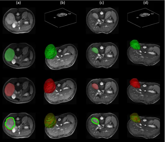
Fig. 5: Segmentation results. Column (a): 2D images before radio-chemotherapy, green the segmentation result, red the hand-labelled and the overlap of both images. Column (b): corresponding 3D images before radio-chemotherapy, green the segmentation result, red the hand-labelled and the overlap of both images. Column (c): 2D images after radio-chemotherapy, green the segmentation result, red the hand-labelled and the overlap of both images. Column (d): corresponding 3D images after radio-chemotherapy, green the segmentation result, red the hand-labelled and the overlap of both sans.

Fig. 6: Illustration of the importance of our semi-automatic segmentation method from selected slices in the 3D scan: (a) Input scan with ill-defined boundary. (b) our segmentation result, (c) the hand-labelled image.

CONCLUSION

In summary, we have developed a semi-automated method to extract Wilms’ tumour from multi-sequence MRI scans. The method has been designed, tested and validated in conjunction with medical experts, enabling its deployment and exploitation in the clinical setting. The overall procedure includes a pre-processing step that enhances the contrast of the tumour in a multi-sequence scan using a bias correction operation, and a tumour extraction step that includes kernel mapping and continuous max-flow algorithm. The method was validated on 48 multi-sequence MRI scans and it is proved to be accurate, robust, flexible, and fast, leading to a successful extraction of the tumour tissue. Our method has the advantage over fully automated segmentation methods because it allows an easy interaction of the user with different slices and facilitates the

learning methodologies would refine and personalise the evaluation of patient imaging data.

REFERENCES

Adams R, Bischof L (1994). Seeded region growing. IEEE Transactions on Pattern Analysis and Machine Intelligence 16:641–7.

Amiri S, Rekik I, Mahjoub MA (2016). Deep random forest-based learning transfer to svm for brain tumor segmentation. In: 2016 2nd International Conference on Advanced Technologies for Signal and Image Processing (ATSIP).

Bauer S, Fejes T, Slotboom J, Wiest R, Nolte LP, Reyes M (2012). Segmentation of brain tumor images based on integrated hierarchical classification and regularization. In: MICCAI BraTS Workshop. Nice: Miccai Society.

Bauer S, Wiest R, Nolte LP, Reyes M (2013a). A survey of MRI-based medical image analysis for brain tumor studies. Physics in medicine and biology 58:R97–129.

Bauer S, Wiest R, Nolte LP, Reyes M (2013b). A survey of MRI-based medical image analysis for brain tumor studies. Physics in medicine and biology 58:R97–129.

Boykov Y, Funka-Lea G (2006). Graph cuts and efficient nd image segmentation. International journal of computer vision 70:109–31.

Boykov YY, Jolly MP (2001). Interactive graph cuts for optimal boundary & region segmentation of objects in nd images. In: Computer Vision, 2001. ICCV 2001. Proceedings. Eighth IEEE International Conference on, vol. 1. IEEE.

Chen X, Udupa JK, Bagci U, Zhuge Y, Yao J (2012). Medical image segmentation by combining graph cuts and oriented active appearance models. IEEE Transactions on Image Processing 21:2035–46. Conze P, Noblet V, Rousseau F, Heitz F, Memeo

R, Pessaux P (2016). Random forests on hierarchical multi-scale supervoxels for liver tumor segmentation in dynamic contrast-enhanced ct scans. In: 2016 IEEE 13th International Symposium on Biomedical Imaging (ISBI). David R, Graf N, Karatzanis I, Stenzhorn H, Manikis

G, Sakkalis V, Stamatakos G, Marias K (2012). Clinical evaluation of DoctorEye platform in nephroblastoma. Proceedings of the 2012 5th International Advanced Research Workshop on In Silico Oncology and Cancer Investigation The TUMOR Project Workshop IARWISOCI 2012 . Esneault S, Hraiech N, Delabrousse ´E, Dillenseger

JL (2007). Graph cut liver segmentation

for interstitial ultrasound therapy. Annual International Conference of the IEEE Engineering in Medicine and Biology Proceedings :5247–50. Farmaki C, Marias K, Sakkalis V, Graf N (2010).

Spatially Adaptive Active Contours: A Semi-Automatic Tumor Segmentation Framework. International journal of computer assisted radiology and surgery 5:369–84.

Freedman D, Zhang T (2005). Interactive graph cut based segmentation with shape priors. In: 2005 IEEE Computer Society Conference on Computer Vision and Pattern Recognition (CVPR’05), vol. 1. Goceri N, Goceri E (2015). A neural network based kidney segmentation from mr images. In: 2015 IEEE 14th International Conference on Machine Learning and Applications (ICMLA).

Gordillo N, Montseny E, Sobrevilla P (2013). State of the art survey on MRI brain tumor segmentation. Magnetic Resonance Imaging 31:1426–38. Gu L, Xu J, Peters TM (2006). Novel multistage

three-dimensional medical image segmentation: methodology and validation. IEEE transactions on information technology in biomedicine a publication of the IEEE Engineering in Medicine and Biology Society 10:740–8.

Ju W, Xiang D, Zhang B, Wang L, Kopriva I, Chen X (2015). Random walk and graph cut for co-segmentation of lung tumor on pet-ct images. IEEE Transactions on Image Processing 24:5854– 67.

Kaba D, Wang Y, Wang C, Liu X, Zhu H, Salazar-Gonzalez aG, Li Y (2015). Retina layer segmentation using kernel graph cuts and continuous max-flow. Optics express 23:7366–84. Kainm¨uller D, Lange T, Lamecker H (2007). Shape constrained automatic segmentation of the liver based on a heuristic intensity model. In: Proc. MICCAI Workshop 3D Segmentation in the Clinic: A Grand Challenge.

Kim DY, Park JW (2004). Computer-Aided Detection of Kidney Tumor on Abdominal Computed Tomography Scans. Acta Radiologica 45:791–5. Lee CH, Wang S, Murtha A, Brown MR, Greiner R

(2008). Segmenting brain tumors using pseudo— conditional random fields. In: Proceedings of the 11th International Conference on Medical Image Computing and ComputerAssisted Intervention -Part I, MICCAI ’08. Berlin, Heidelberg: Springer-Verlag.

Contrast-Enhanced Abdominal CT. Pattern recognition 42:1149–61.

Liu B, Cheng HD, Huang J, Tian J, Tang X, Liu J (2010). Fully automatic and segmentation-robust classification of breast tumors based on local texture analysis of ultrasound images. Pattern Recognition 43:280–98.

Mancas M, Gosselin B (2003). Fuzzy tumor segmentation based on iterative watersheds. Proc of the 14th ProRISC workshop on Circuits Systems and Signal Processing ProRISC 2003 Veldhoven Netherland :5.

McInerney T, Terzopoulos D (1996). Deformable models in medical image analysis: a survey. Medical image analysis 1:91–108.

Menze BH, Jakab A, Bauer S, Kalpathy-Cramer J, Farahani K, Kirby J, Burren Y, Porz N, Slotboom J, Wiest R, Lanczi L, Gerstner E, Weber M, Arbel T, Avants BB, Ayache N, Buendia P, Collins DL, Cordier N, Corso JJ, Criminisi A, Das T, Delingette H, Demiralp , Durst CR, Dojat M, Doyle S, Festa J, Forbes F, Geremia E, Glocker B, Golland P, Guo X, Hamamci A, Iftekharuddin KM, Jena R, John NM, Konukoglu E, Lashkari D, Mariz JA, Meier R, Pereira S, Precup D, Price SJ, Raviv TR, Reza SMS, Ryan M, Sarikaya D, Schwartz L, Shin H, Shotton J, Silva CA, Sousa N, Subbanna NK, Szekely G, Taylor TJ, Thomas OM, Tustison NJ, Unal G, Vasseur F, Wintermark M, Ye DH, Zhao L, Zhao B, Zikic D, Prastawa M, Reyes M, Leemput KV (2015). The multimodal brain tumor image segmentation benchmark (brats). IEEE Transactions on Medical Imaging 34:1993–2024. Pham DL, Xu C, Prince JL (2000). Current Methods in

Medical Image Segmentation. Annu Rev Biomed Eng 2:315–37.

Ramrez I, Martn A, Schiavi E (2018). Optimization of a variational model using deep learning: An application to brain tumor segmentation. In: 2018 IEEE 15th International Symposium on Biomedical Imaging (ISBI 2018).

Sachdeva J, Kumar V, Gupta I, Khandelwal N, Ahuja CK (2012). A novel content-based active contour model for brain tumor segmentation. Magnetic Resonance Imaging 30:694–715.

Salah MB, Ayed IB, Yuan J, Zhang H (2014). Convex-relaxed kernel mapping for image segmentation. IEEE Transactions on Image Processing 23:1143– 53.

Salah MB, Mitiche A, Ayed IB (2011). Multiregion image segmentation by parametric kernel graph cuts. IEEE Transactions on Image Processing 20:545–57.

Salazar-Gonzalez A, Kaba D, Li Y, Liu X (2014). Segmentation of Blood Vessels and Optic Disc in Retinal Images. IEEE Journal of Biomedical and Health Informatics 2194:1–.

Sauwen N, Sima DM, Acou M, Achten E, Maes F, Himmelreich U, Huffel SV (2016). A semi-automated segmentation framework for mri based brain tumor segmentation using regularized nonnegative matrix factorization. In: 2016 12th International Conference on Signal-Image Technology Internet-Based Systems (SITIS). Shah N, Ziauddin S, Shahid AR (2017). Brain

tumor segmentation and classification using cascaded random decision forests. In: 2017 14th International Conference on Electrical Engineering/Electronics, Computer, Telecommunications and Information Technology (ECTI-CON).

Somaskandan S, Mahesan S (2012). A level set based deformable model for segmenting tumors in medical images. In: International Conference on Pattern Recognition, Informatics and Medical Engineering (PRIME-2012).

Stamatakos G, Graf N (2017). Computational horizons in cancer (chic). Clinical Therapeutics 39:e107– e108.

Tustison NJ, Avants BB, Cook PA, Zheng Y, Egan A, Yushkevich PA, Gee JC (2010). N4ITK: improved N3 bias correction. IEEE transactions on medical imaging 29:1310–20.

van der Lijn F, den Heijer T, Breteler MMB, Niessen WJ (2008). Hippocampus segmentation in mr images using atlas registration, voxel classification, and graph cuts. NeuroImage 43:708–20.

Wang T, Cheng I, Basu A (2009). Fluid vector flow and applications in brain tumor segmentation. IEEE transactions on biomedical engineering 56:781–9. Yuan J, Bae E, Tai XC (2010). A study on continuous

max-flow and min-cut approaches. Proceedings of the IEEE Computer Society Conference on Computer Vision and Pattern Recognition :2217– 24.

Zhan Y, Shen D (2006). Deformable segmentation of 3-d ultrasound prostate images using statistical texture matching method. IEEE Transactions on Medical Imaging 25:256–72.