Astronomy
&
Astrophysics
https://doi.org/10.1051/0004-6361/201732378© ESO 2018
Magnetic fields at the onset of high-mass star formation
H. Beuther
1, J. D. Soler
1, W. Vlemmings
2, H. Linz
1, Th. Henning
1, R. Kuiper
3,
R. Rao
4, R. Smith
5, T. Sakai
6, K. Johnston
7, A. Walsh
8, and S. Feng
91Max Planck Institute for Astronomy, Königstuhl 17, 69117 Heidelberg, Germany
e-mail:beuther@mpia.de
2Department of Earth and Space Sciences Chalmers University of Technology, Onsala Space Observatory, 439 92 Onsala, Sweden
3Institute of Astronomy and Astrophysics, University of Tübingen, Auf der Morgenstelle 10, 72076 Tübingen, Germany
4Academia Sinica Institute of Astronomy and Astrophysics, 645 N. Aohoku Place, Hilo, HI 96720, USA
5School of Physics and Astronomy, University of Manchester, Oxford Road, Manchester M13 9PL, UK
6Department of Communication Engineering and Informatics, The University of Electro-Communications, Chofugaoka, Chofu,
Tokyo 182-8585, Japan
7School of Physics and Astronomy, University of Leeds, Leeds LS2 9JT, UK
8International Centre for Radio Astronomy Research, Curtin University, GPO Box U1987, Perth, WA 6845, Australia
9Max-Planck-Institut für Extraterrestrische Physik, Giessenbachstrasse 1, 85748 Garching, Germany
Received 28 November 2017 / Accepted 29 January 2018
ABSTRACT
Context. The importance of magnetic fields at the onset of star formation related to the early fragmentation and collapse processes is largely unexplored today.
Aims. We want to understand the magnetic field properties at the earliest evolutionary stages of high-mass star formation.
Methods. The Atacama Large Millimeter Array is used at 1.3 mm wavelength in full polarization mode to study the polarized emission, and, using this, the magnetic field morphologies and strengths of the high-mass starless region IRDC 18310-4.
Results. Polarized emission is clearly detected in four sub-cores of the region; in general it shows a smooth distribution, also along elongated cores. Estimating the magnetic field strength via the Davis-Chandrasekhar-Fermi method and following a structure function analysis, we find comparably large magnetic field strengths between∼0.3–5.3 mG. Comparing the data to spectral line observations, the turbulent-to-magnetic energy ratio is low, indicating that turbulence does not significantly contribute to the stability of the gas clump. A mass-to-flux ratio around the critical value 1.0 – depending on column density – indicates that the region starts to collapse, which is consistent with the previous spectral line analysis of the region.
Conclusions. While this high-mass region is collapsing and thus at the verge of star formation, the high magnetic field values and the smooth spatial structure indicate that the magnetic field is important for the fragmentation and collapse process. This single case study can only be the starting point for larger sample studies of magnetic fields at the onset of star formation.
Key words. stars: formation – instrumentation: interferometers – magnetic fields – polarization – stars: individual: IRDC18310 – ISM: clouds
1. Introduction
The importance of magnetic fields during the formation of stars has been the topic of great controversy over the last decades. While some groups stress that magnetic fields are of utmost importance during cloud formation and core collapse processes (e.g.,Mouschovias & Paleologou 1979;Mouschovias et al. 2006;
Commerçon et al. 2011;Peters et al. 2011;Tan et al. 2013;Tassis et al. 2014; Myers et al. 2013, 2014), others consider that the effects of turbulence and gravity are far more important for gov-erning star formation (e.g.,Padoan & Nordlund 2002; Klessen et al. 2005;Vázquez-Semadeni et al. 2011). Even the interpreta-tion of a single dataset can be extremely controversial regarding the importance of magnetic fields (e.g.,Mouschovias & Tassis 2009;Crutcher et al. 2010).
More specifically, at the onset of collapse during the forma-tion of high-mass clusters, observaforma-tions show that gas clumps fragment, although, on average, less than predicted by classi-cal Jeans fragmentation (e.g., Wang et al. 2014;Beuther et al. 2015;Zhang et al. 2015;Fontani et al. 2016). Different processes
are able to explain the suppressed fragmentation of the initial gas clumps, in particular steep initial density structures (e.g.,
Girichidis et al. 2011), turbulence (e.g., Wang et al. 2014) or magnetic fields (e.g.,Commerçon et al. 2011;Fontani et al. 2016;
Klassen et al. 2017).
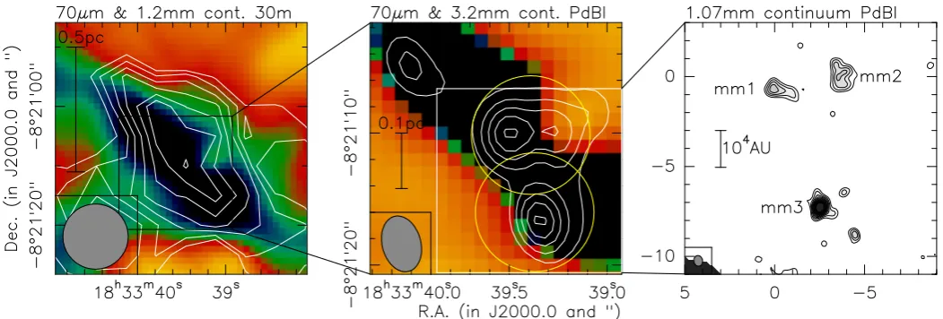
Fig. 1.Compilation of the continuum images in IRDC 18310-4 (Beuther et al. 2013,2015). Theleftandmiddle panelsshow in color theHerschel
70µm image with a stretch going dark for low values. The white contours in theleft panelshow the 1.2 mm MAMBO continuum observations starting from 4σand continuing in steps of 1σ,with 1σbeing equal to 13 mJy beam−1. The contours in themiddle panelpresents the 3.2 mm PdBI continuum data starting from 3σand continuing in steps of 2σ,with 1σequal to 0.08 mJy beam−1. The two yellow circles outline the∼900
inner third of the two pointings (field 1 north, field 2 south) we observed in this polarization project. Theright panelthen shows the 1.07 mm PdBI continuum observations starting from 3σand continuing in steps of 1σwith 1σequal to 0.6 mJy beam−1.
(Beuther et al. 2013, 2015). The fragment separations in that region are consistent with thermal Jeans fragmentation; however, the core masses are more than an order of magnitude larger than the typical Jeans mass (Beuther et al. 2015). They suggest that these discrepancies can be reconciled by invoking either non-homogeneous initial density structures or strong magnetic fields. Here, we investigate the magnetic field properties of the region.
2. Observations
The infrared dark cloud IRDC18310-4 was observed with the Atacama Large Millimeter Array (ALMA) as a cycle 3 project (2015.1.00492.S) during four sessions between June 17 and June 20, 2016. The observations were conducted in the 1 mm band with the predefined frequency setting as it was at that time for ALMA polarization observations, with the LO at 233 GHz to avoid any strong line contamination. The four basebands with 2 GHz bandwidth were each centered at 224, 226, 240 and 242 GHz. The channel width was 31.25 MHz. At this frequency, the primary beam of the ALMA 12 m array is 2700, in principle large enough to encompass our region of interest. However, taking into account that ALMA still recommends that only the inner third of the primary beam is reliable for polarization measurements, we used two fields centered on the main contin-uum sources as shown in Fig.1. The two corresponding phase centers are for field 1 RA (J2000.0) 18:33:39.4, Dec (J2000.0) -08:21:10.2, and for field 2 RA (J2000.0) 18:33:39.4, Dec (J2000.0) -08:21:16.0, separated by only 5.800in declination. Two slightly different array configurations were used (C36-2, C36-3) with a total baseline range of between 15 and 704 m. The shortest baseline would correspond theoretically to maximum recoverable scales of approximately 2200. However, typically such theoretical limits are not achieved in interferometric imaging because of the weighting of data and missing baselines also at intermediate scales. ALMA reports for the given con-figurations maximum recoverable scales of∼1100 at 230 GHz1. Hence, large-scale flux is still filtered out, which is quantified in
1 https://almascience.eso.org/observing/
prior-cycle-observing-and-configuration-schedule
the following section. Eight executions (two per session) of the same scheduling block were conducted with on average 35 good antennas in the array. The execution times per scheduling block varied between 85 and 99 min, and the on-source integration time for each observed field was ∼17.6 min per execution. Bandpass calibration was conducted with observations of the quasar J1751+0939 whereas the absolute flux was calibrated with J1733-1304 or Titan. The absolute flux uncertainty should be around 10%. To calibrate phases and amplitudes, regularly interleaved observations of the quasar J1912-0804 were used. The polarization calibration was conducted with J1743-0350.
Calibration and imaging of the data was done in CASA version 4.7. For the calibration we followed the provided pro-cedures from the ALMA observatory. Because the two target fields are so closely spaced, we want to combine them in a single image. However, since the main sub-structures are partly out-side the recommended inner third of the primary beam (Fig.1), tests of the individually imaged fields and combined images were conducted. Figure2 shows the linearly polarized images of the region for each of the two fields separately as well as for the combined dataset. The structures between the two indi-vidually imaged fields agree well, and the combined image has the expected lower noise levels. We conducted an additional test following the approach outlined inMatthews et al. (2014) where the residuals of the linearly polarized QandU compo-nents (Qres & andUres) are calculated first. Then the combined
image (pQ2+U2) is compared to the residual image to gauge
the trustworthiness of the combination. In practice we calculated
Qres=(Q1−Q2)/2 & Ures=(U1−U2)/2 (1)
Mask= p
Q2+U2
3×pQ2res+U2res
. (2)
Fig. 2. Comparison of the images of the two fields, shown both individually and then combined. Theleft panelshows the linearly polarized emission using only field 1, the second panel presents the same emission but using only field 2, and thethird panelshows the combined image. The contour levels are always chosen as the 4σlevels of the combined image where 1σis 6µJy beam−1. Theright panelpresents the mask created from the combined image and the residuals of each individual image followingMatthews et al.(2014); see Sect.2. The contour level is set to 1, corresponding to the 3σconfidence level inMatthews et al.(2014). The beam sizes are shown at the bottom-left of each panel, and the combined image also shows a scale bar.
Fig. 3.Polarization data at 1.3 mm wavelength for IRDC18310-4. Theleft panelshows the Stokes I emission (4σcontours of 0.6 mJy beam−1), and themiddle panelpresents the linearly polarized emission (4σcontours of 24µJy beam−1). The line segments show the corresponding polarization angles (the magnetic field should be rotated by 90◦
). Theright panelshows for comparison the polarization fraction in color with the same contours of linearly polarized emission as in themiddle panel. The polarization fraction should be considered as an upper limit because StokesImay be more strongly affected by interferometric spatial filtering than the weaker polarized emission.
are several times above the 3σ value calculated here, showing again that the combination of the two fields is a valid approach.
Based on these tests, we imaged both datasets together in a mosaic mode with natural weighting and a small uv-taper on the longer baselines to increase our signal-to-noise ratio. All four spectral windows were used for the imaging process. The syn-thesized beam of these images is 1.0100×0.8300 (PA 89◦). The 1σrms values of the Stokes I and the linear polarized image are 0.15 mJy beam−1and 6µJy beam−1, respectively.
3. Results
The following analysis is based on the combined dataset of both observed fields. Figure3 presents an overview of the obtained
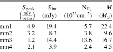
data. The left panel shows the StokesIimage of the region, and we clearly re-identify the three main continuum peaks known from the previous PdBI observations (Fig.1). In addition to these main sources, the more sensitive ALMA data identify additional dust continuum sources in the field. Particularly strong is the south-western source mm4, whereas some weaker features are found between mm2 and mm3 as well as at the north-eastern edge of the field. We concentrate our study of the linearly polar-ized emission on the four strongest sources, mm1 to mm4. The peak (Speak) and integrated fluxes (Sint) within the 4σ
con-tours are shown in Table1. The total integrated flux density of the whole region recovered in the Stokes Iimage of Fig. 3 is 72 mJy beam−1. For comparison, the single-dish 1.2 mm
[image:3.595.37.559.331.551.2]Table 1.Source parameters.
Speak Sint NH2 M
mJy beam
(mJy) (1023cm−2) (M)
mm1 4.9 19.4 5.7 22.4
mm2 3.2 8.3 3.8 9.6
mm3 1.2 14.4 13.6 16.7
mm4 2.1 3.9 2.4 4.5
IRAM 30 m telescope (Beuther et al. 2002) within the inner 1100beam size is 132 mJy, and the 1.2 mm single-dish MAMBO flux density measured within the ALMA primary beam area is
∼410 mJy. Taking into account that there is a slight difference in the observed wavelength between the 1.2 mm single-dish and the 1.3 mm of the ALMA data, approximately 20–50% of the total flux is recovered by our interferometer observations. Assuming optically thin dust emission and following the approach already used inBeuther et al.(2013,2015) we can calculate the H2
col-umn densities (NH2) and gas masses for the four sub-regions.
With gas temperatures in this starless core around∼15 K, a gas-to-dust mass ratio of 150 (Draine 2011), and a dust opacity index
κdiscussed inOssenkopf & Henning(1994) for grains with thin ice mantles at densities of 106cm−3 (κ1.3mm ∼0.9 cm2g−1), the
derived column densities and masses are presented in Table 1. With the main uncertainties in the dust model and the tem-perature, we estimate the accuracy of the masses and column densities within a factor 2. The core masses range between roughly 4 and 22M and the H2 column densities between
2.4×10²³ and 1.36×1024cm−2, consistent with the previous
findings inBeuther et al.(2015).
More importantly for the magnetic field investigation, the middle panel of Fig. 3 presents the linearly polarized emis-sion from the region. All four main mm continuum sources are clearly detected in the polarized emission. Figure3also presents the observed polarization angles, and within each of the four cores, the polarization angles exhibit a relatively ordered struc-ture. While for the more compact sources, mm3 and mm4, less independent polarization angle measurements are possible; the orientation in the two sources is roughly northeast-southwest and east-west, respectively. For the more extended sources mm1 and mm2, the polarization angle distribution shows some smooth angle shifts over the extent of the structures. The well-structured polarization angles are already a first indication that the mag-netic field may be important in that region because turbulence-dominated regions would show less structured polarization angle distributions. We also do not see signs of polarization holes toward the peak positions like those observed previously toward low-mass star-forming regions (e.g., Wolf et al. 2003; Hull et al. 2014). However, the fact that the mean polarization angles toward the four main mm sources are very different may be one explanation for the polarization holes sometimes observed in single-dish data (e.g.,Matthews et al. 2009). Single-dish obser-vations would average over the polarization properties of the four sub-sources which could result in a lowered signal toward the lower-resolution single-dish data. In addition to this, the right panel in Fig.3presents the corresponding polarization fraction, and we find values typically between 1 and 10%. The latter high values should be considered as upper limits because the much stronger Stokes I emission, that may come from comparably larger scales, may be more strongly affected by interferomet-ric spatial filtering than the weaker polarized emission. While
we can measure the missing flux for Stokes I (see above), we do not have the single-dish information for the linearly polar-ized emission. Hence, we cannot conclusively answer how much missing flux differences between polarized and non-polarized emission may affect the polarization fraction measurement. For comparison, in their TADPOL magnetic field study of 30 mainly low-mass star-forming regions (with a few high-mass, more evolved regions included), Hull et al.(2014) measured typical polarization fractions between 1 and ∼8%, largely consistent with our measurement. However, at 2.500they also find regularly polarization holes toward the peak positions which is not evident in our data. This indicates that at the scales resolved here for IRDC 18310-4, the magnetic field structure is still largely ordered and coherent.
4. Magnetic fields
4.1. Magnetic field strength via Davis-Chandrasekhar-Fermi method
The Davis-Chandrasekhar-Fermi method (hereafter the DCF,
Davis 1951;Chandrasekhar & Fermi 1953) can be used to calcu-late the magnetic field strength in a gas if the angular dispersion of the local magnetic field orientations,σψ, the gas density,ρ, and the one (1D) velocity dispersion of the gas,σv, are known. Assuming that the magnetic field is frozen into the gas and that the dispersion of the local magnetic field orientation angles is due to transverse and incompressible Alfvén waves, then the strength of the plane-of-the-sky component of the magnetic field is
BDCF⊥ = p
4πρσv
σψ. (3)
We calculate BDCF⊥ using the procedure described in Appendix D of Planck Collaboration Int. XXXV (2016). We estimateρassuming an average number densityn =106cm−3
(Beuther et al. 2013) and a mean molecular weight µ = 2.8mp, where mp is the proton mass. The 1D velocity
dis-persion, σv, is estimated from the width of the N2H+ line
measured in this region (Beuther et al. 2015). With a line width∆v(N2H+)∼0.3 km s−1, we getσv≈∆v(N2H+)/
√
8ln2≈
0.3km s−1/√8ln2≈0.13 km s−1. Because more accurate,
indi-vidual estimates per core are difficult, we use the same value ofσvandnfor all three sub-regions. We estimate the values of the angular dispersion of the local magnetic field orientations directly from the StokesQandUby using
σψ=
q
(∆ψ)2, (4)
where
∆ψ=0.5×arctan QhUi − hQiU QhQi − hUiU !
, (5)
andh· · · idenotes an average over the selected pixels in each map. The angular dispersions of the polarization vectors as well as the derived magnetic field values are presented in Table 2 for mm1 to mm3 (mm4 is too close to a point source for reasonable estimates). On average we find comparably high magnetic field values in the several hundredµG to mG regime.
Table 2.Magnetic field strength estimates.
Source σψ BDCF
⊥ b(0) BS F⊥
[deg] [mG] [deg] [mG]
mm1 17.9 0.3±0.1 1.1 5.3±2.6
mm2 10.1 0.6±0.2 6.4 0.9±0.3
[image:5.595.43.285.99.317.2]mm3 4.3 1.3±0.4 3.8 1.5±0.5
Fig. 4.Histogram of polarization orientation angles,ψ, towards each of the sources.
source and hence dominated by beam effects. One should keep in mind that the absolute errors for the Davis-Chandrasekhar-Fermi method are even larger because of its underlying assumptions and the effect of projection and line-of-sight integration, which are discussed in detail in Appendix D ofPlanck Collaboration Int. XXXV (2016). For example, it is difficult to determine whether the measured dispersion around the mean field σψ is exclusively the effect of magneto-hydrodynamic waves and tur-bulence. Moreover, the observed value ofσψ is an average of various magnetic field vectors, and integration of multiple com-ponents along the line may decrease the measurable polarization angle compared to the true dispersion of the magnetic field orientation. Furthermore, the velocity dispersion estimates are obtained using a tracer that does not necessarily sample the same volume as traced by the dust polarization. Finally, the mean densities are assumed, whereas density gradients exist within each region. In summary, the magnetic field estimates from the Davis-Chandrasekhar-Fermi method should be considered as order-of-magnitude estimates, which are illustrative of the dif-ferences between the regions, but do not fully encompass the complexity of the field dynamics in each one of them.
4.2. Structure function of the polarization orientation angles
In dense clouds, the magnetic field structure is the result of multiple physical processes not accounted for by the basic DCF analysis. Consequently, dispersion measured for mean fields that are assumed to be straight may be much larger than should be attributed to magneto-hydrodynamical waves or turbulence. In the region IRDC 18310-4, the distribution of polarization orien-tation angles, illustrated in Fig.4, shows that in sources mm1 and mm2 there is broad distribution or two separate components of polarization orientations, which could lead to an overestimation ofσψand, correspondingly, an underestimation ofBDCF⊥ .
FollowingHildebrand et al.(2009) andHoude et al.(2009,
2011), we can analyze the structure function (of second order) S2(`), also known as the dispersion function, of the
polariza-tion angles. This structure funcpolariza-tion essentially measures the
Fig. 5.Structure function of the polarization orientation angles,S2(`), towards each of the sources. The dashed lines correspond to the fit to the values ofS2(`) in the range` >0.400.
differences between polarization angles separated by displace-ments`. Large values inS2reflect large variations whereas small
values indicate less dispersion between measured polarization angles. This structure function of the polarization orientation angles S2(`) allows for the evaluation of the dispersion of
polarization angles,σψ, while avoiding the effect of large-scale non-turbulent perturbations (Hildebrand et al. 2009). The evalu-ation ofσψis made by fitting the square of the structure function of polarization angles,S2(`), with a second-order polynomial, S22(`)=b(`)+a02`2 , above length scales that are dominated by the beam; in this case we chose to fit for` > 0.400. Evaluating the interceptb(0) of that fit gives an alternative measure for the dispersion of polarization angles (Table2).
It is evident from the values ofS2(`) presented in Fig.5that
the three sources have very different behaviors. In the case of source mm3, the available data does not allow us to extend the study of S2(`) to `-values larger than the size of synthesized
beam, thus it seems to be dominated by the interferometer res-olution. In the case of source mm2, the values ofS2(`) lead to
a value ofb(0) that is comparable to the values ofσψ estimated using Eq. (4), suggesting that despite the two peaks in the ori-entation angle distribution, the assumption of a single straight mean magnetic field direction is not too inadequate for this region.
The case of source mm1 is, however, very different from that of mm2 or mm3. For mm1, the relatively large values of σψ reflects the broad orientation angle distribution, but in contrast to mm2, the valueS2(`) of the dispersion of polarization
orien-tation angles that can be directly attributed to turbulence is very small, that is,b(0)=1.1. This indicates that in mm1, the mean magnetic field direction is not straight and that despite the con-clusions that can be drawn from the simple DCF, the magnetic field must be comparatively stronger. The values of the magnetic field strengths based on the angle dispersions calculated from S2(`),BS F⊥ are also summarized in Table2.
4.3. Magnetic field implications
With an approximate mean magnetic field strength in the plane of the sky of 2.6 mG (BS F⊥ values in Table2) and a typical den-sity of 106cm−3 (Beuther et al. 2013), the 1D Alfven velocity isσA=B/
p
4πρ∼3.4 km s−1. In the following we assume that
the whole maternal clump of ∆v ∼1.5 km s−1 (Beuther et al. 2013), the corresponding 1D velocity dispersion is∼0.64 km s−1.
These numbers indicate that any turbulent or infall velocity is below the Alfvenic velocity. Following Girart et al. (2009) or
Beuther et al.(2010), we can estimate the ratio of turbulent-to-magnetic energy asβ∼3(σv/σA)2. Using the larger line-of-sight
velocity dispersion of the whole clump results in a turbulent-to-magnetic energy ratio ofβ≈0.1,whereas the lower σv for the individual cores would result inβ≈0.004. Hence, for this high-mass starless region, the magnetic energy appears to dom-inate over the turbulent energy and thus should be an important ingredient for the formation of high-mass stars.
In our previous study of the region (Beuther et al. 2015), we discussed whether thermal Jeans fragmentation could explain the general fragmentation properties of the region or whether an adapted turbulent Jeans fragmentation may be more likely. While the fragment separations were found to be consistent with ther-mal Jeans fragmentation, the fragment masses are much higher than the thermal predictions (Beuther et al. 2015). Although tur-bulent Jeans fragmentation could explain the higher masses, the fact that the measured line widths toward individual cores are so small (Beuther et al. 2015) does make the turbulent interpre-tation less likely. In that context, it is interesting to investigate how the magnetic field affects such estimates. If one replaces the thermal sound speed at the given low temperatures of∼15 K with the Alfven velocity estimated above, the estimated length scales rise by up to a factor 20, and the estimated masses by even the cube of that. Such high separations and masses exceed the observed values (Beuther et al. 2015). Hence, while the mag-netic field definitely influences the fragmentation of the region, such a simplified “magnetic Jeans fragmentation” picture cannot explain the observed data alone.
A different way to gauge the stability of a region is the mass-to-flux ratio M/ΦB ≈7.6×10⁻²⁴
NH2
B that is given in units of
the critical mass-to-flux ratio (M/ΦB)crit (with NH2 and B in
cm−2and mG;Crutcher 1999;Troland & Crutcher 2008). Using
the average magnetic field of ∼2.6 mG and the column den-sityNH2 ∼1.3×10
23cm−2observed on larger-scales (1100) with
single-dish instruments (Beuther et al. 2013), we get a mass-to-flux ratio M/ΦB of ∼0.4. This is likely a lower limit because
it may well be that the magnetic field strength on larger spa-tial scales could be lower than what we measure at the higher inner densities. Using the higher average column densities from these ALMA observations NH2,av ∼ 8.2×1023cm−2, one gets M/ΦB ∼2.4. This indicates that while on large scales the
over-all gas clump may still be at the verge of criticality, on smover-aller scales it should be collapsing. Such early collapse motions are also inferred from the spectral line data inBeuther et al.(2015).
5. Discussion and conclusions
To the authors knowledge, this is the first high-spatial-resolution magnetic field study of a very young high-mass star-forming region at the onset of collapse prior to any signpost of star formation. For more evolved regions hosting high-mass proto-stellar objects and/or hot molecular cores, the findings about the importance of the magnetic field are ambiguous. While for some regions the magnetic field should play a dominant role (e.g., G31.4, W75N, W51 or CepA; Girart et al. 2009; Surcis et al. 2009;Tang et al. 2009;Vlemmings et al. 2010), other sys-tems appear to be more strongly influenced by dynamic motions (e.g., IRAS 1809-1732;Beuther et al. 2010). The magnetic field values estimated for IRDC 18310-4 on the order of ∼2.6 mG
are lower or around what is found for several more evolved hot-core-like regions; for example, W3(H2O), IRAS 18089-1732
or NGC7538IRS1 with reported values of 17, 11, and 2.5 mG, respectively (Chen et al. 2012; Beuther et al. 2010;Frau et al. 2014). With only one high-mass starless region observed so far, this difference is not yet conclusive, but it will be interesting to see with future data whether or not the measured magnetic field strengths are indeed related to the evolutionary stage.
Our findings for this high-mass starless region that the mass-to-flux ratio is of order unity (depending on the column density) and at the same time that the turbulent-to-magnetic energy ratio is comparably low are both indications for the general instability of the region. The latter finding mainly implies that turbulence is not contributing significantly to the stability of the region. Nevertheless, stability is not needed because the kinematic sig-natures found byBeuther et al.(2015) already implied that the whole gas clump is globally collapsing and at the verge of star formation. This is consistent with the high mass-to-flux ratio. The mean magnetic field strength around∼2.6 mG does not con-tradict that picture; it simply implies that the magnetic field significantly contributes to the fragmentation and collapse prop-erties of the overall gas clump. For example, high magnetic field values can inhibit fragmentation into many low-mass cores (e.g., Commerçon et al. 2011; Peters et al. 2011; Myers et al. 2013,2014;Fontani et al. 2016). For IRDC 18310-4, even at the higher resolution of the previous PdBI observations, several of the cores do not fragment but show masses in excess of 10M (Beuther et al. 2015). Although the sensitivity of these data is not sufficient to detect cores below 1M, the fact that massive non-fragmenting cores at the given spatial resolution are identi-fied, is indicative of large magnetic fields that we observe now with the new ALMA data. The overall smooth spatial structure of the polarization angles is additional evidence for the dynamic importance of the magnetic field.
In summary, while the maternal gas clump is collapsing at large, the polarization data reveal that the magnetic field is important for the fragmentation and star formation process in this region. However, a single case study is not sufficient for a general conclusion, and it can only set the stage for future studies of larger samples.
Acknowledgements. This paper makes use of the following ALMA data: ADS/JAO.ALMA#2015.1.00492.S. ALMA is a partnership of ESO (representing its member states), NSF (USA) and NINS (Japan), together with NRC (Canada) and NSC and ASIAA (Taiwan) and KASI (Republic of Korea), in cooperation with the Republic of Chile. The Joint ALMA Observatory is operated by ESO, AUI/NRAO and NAOJ. HB and JDS acknowledge support from the European Research Council under the Horizon 2020 Framework Program via the ERC Consolidator Grant CSF-648505. WV acknowledges funding from the European Research Council under the European Union’s Seventh Framework Programme (FP/2007-2013) / ERC Grant Agreement n. 614264. RK acknowledges financial support from the German Research Foundation (DFG) under the Emmy Noether Research Program via the grant no. KU 2849/3-1. RS acknowledges support from the STFC through an Ernest Rutherford Fellowship.
References
Beuther, H., Schilke, P., Menten, K. M., et al. 2002,ApJ, 566, 945
Beuther, H., Vlemmings, W. H. T., Rao, R., & van der Tak, F. F. S. 2010,ApJ, 724, L113
Beuther, H., Linz, H., Tackenberg, J., et al. 2013,A&A, 553, A115
Beuther, H., Henning, T., Linz, H., et al. 2015,A&A, 581, A119
Chandrasekhar, S., & Fermi, E. 1953,ApJ, 118, 113
Chen, H.-R., Rao, R., Wilner, D. J., & Liu, S.-Y. 2012,ApJ, 751, L13
Commerçon, B., Hennebelle, P., & Henning, T. 2011,ApJ, 742, L9
Crutcher, R. M., Wandelt, B., Heiles, C., Falgarone, E., & Troland, T. H. 2010,
ApJ, 725, 466
Davis, L. 1951,Phys. Rev., 81, 890
Draine, B. T. 2011,Physics of the Interstellar and Intergalactic Medium (Prince-ton Series in Astrophysics)
Fontani, F., Commerçon, B., Giannetti, A., et al. 2016,A&A, 593, L14
Frau, P., Girart, J. M., Zhang, Q., & Rao, R. 2014,A&A, 567, A116
Girart, J. M., Beltrán, M. T., Zhang, Q., Rao, R., & Estalella, R. 2009,Science, 324, 1408
Girichidis, P., Federrath, C., Banerjee, R., & Klessen, R. S. 2011,MNRAS, 413, 2741
Hildebrand, R. H., Kirby, L., Dotson, J. L., Houde, M., & Vaillancourt, J. E. 2009,ApJ, 696, 567
Houde, M., Vaillancourt, J. E., Hildebrand, R. H., Chitsazzadeh, S., & Kirby, L. 2009,ApJ, 706, 1504
Houde, M., Rao, R., Vaillancourt, J. E., & Hildebrand, R. H. 2011,ApJ, 733, 109
Hull, C. L. H., Plambeck, R. L., Kwon, W., et al. 2014,ApJS, 213, 13
Klassen, M., Pudritz, R. E., & Kirk, H. 2017,MNRAS, 465, 2254
Klessen, R., Jappsen, K., Larson, R., Li, Y., & Mac Low M.-M. 2005, in The Ini-tial Mass Function 50 Years Later, eds. E. Corbelli, F. Palla, & H. Zinnecker, (Dordrecht, NL: Springer)Astrophys. Space Sci. Lib., 327, 363
Matthews, B. C., McPhee, C. A., Fissel, L. M., & Curran, R. L. 2009,ApJS, 182, 143
Matthews, T. G., Ade, P. A. R., Angilè, F. E., et al. 2014,ApJ, 784, 116
Mouschovias, T. C., & Paleologou, E. V. 1979,ApJ, 230, 204
Mouschovias, T. C., & Tassis, K. 2009,MNRAS, 400, L15
Mouschovias, T. C., Tassis, K., & Kunz, M. W. 2006,ApJ, 646, 1043
Myers, A. T., McKee, C. F., Cunningham, A. J., Klein, R. I., & Krumholz, M. R. 2013,ApJ, 766, 97
Myers, A. T., Klein, R. I., Krumholz, M. R., & McKee, C. F. 2014,MNRAS, 439, 3420
Ossenkopf, V., & Henning, T. 1994,A&A, 291, 943
Padoan, P., & Nordlund, Å. 2002,ApJ, 576, 870
Peters, T., Banerjee, R., Klessen, R. S., & Mac Low M.-M. 2011,ApJ, 729, 72
Planck Collaboration Int. XXXV. 2016,A&A, 586, A138
Sridharan, T. K., Beuther, H., Saito, M., Wyrowski, F., & Schilke, P. 2005,ApJ, 634, L57
Surcis, G., Vlemmings, W. H. T., Dodson, R., & van Langevelde H. J. 2009,
A&A, 506, 757
Tan, J. C., Kong, S., Butler, M. J., Caselli, P., & Fontani, F. 2013,ApJ, 779, 96
Tang, Y., Ho, P. T. P., Koch, P. M., et al. 2009,ApJ, 700, 251
Tassis, K., Willacy, K., Yorke, H. W., & Turner, N. J. 2014,MNRAS, 445, L56
Troland, T. H., & Crutcher, R. M. 2008,ApJ, 680, 457
Vázquez-Semadeni, E., Banerjee, R., Gómez, G. C., et al. 2011,MNRAS, 414, 2511
Vlemmings, W. H. T., Surcis, G., Torstensson, K. J. E., & van Langevelde H. J. 2010,MNRAS, 404, 134
Wang, K., Zhang, Q., Testi, L., et al. 2014,MNRAS, 439, 3275
Wolf, S., Launhardt, R., & Henning, T. 2003,ApJ, 592, 233