RIT Scholar Works
Theses
Thesis/Dissertation Collections
2000
Color tolerance: A comparison of the method of
constant stimuli and the gray scale comaprison
method on a CRT
David Wilbur
Follow this and additional works at:
http://scholarworks.rit.edu/theses
This Thesis is brought to you for free and open access by the Thesis/Dissertation Collections at RIT Scholar Works. It has been accepted for inclusion in Theses by an authorized administrator of RIT Scholar Works. For more information, please [email protected].
Recommended Citation
Color Tolerance:
A comparison of the method of constant stimuli and the gray scale comaprison method on
a CRT
*David C. Wilbur, Ethan Montag
Chester F. Carlson Center for Imaging Science
Rochester Institute of Technology
Rochester, NY 14623-5604
May 2000
Color Tolerance Comparison
David C. Wilbur
Table of Contents
Abstract
Copyright
Acknowledgement
Introduction
Background
Theory
Methods
Results
Discussion
Conclusion
References
Appendix
Color Tolerance: A comparison of the method of constant stimuli and gray
scale comparison method on a CRT.
David C. Wilbur
Abstract
This research compares two psychophysical methods, the method of constant stimuli and the gray scale comparison method. Three color centers were chosen: Red(L*=47.4, a*=61.90, b*=49.5), Green(L*=65.00, a*=-67.6, b*=54.60), and Gray(L*=60, a*=0.00, b*=0,00). Each color center varied in three different directions, L*, C*, and H*. Ten color difference samples were chosen for each color center in each direction, for a total of 30 different samples for the rea and green color centers and 10 samples for the gray color center.
Each method employed the same three color centers. The sample paris were compared with a neutral anchor pair stimulus of 1.0 ?Eab*. In total there are 70 different color difference samples in ech comparison method.
30 observers participated in the experiment where in each experiment they compared 70 different color difference samples in each experiment for a total of 140 observations. The entire experiment consisted of a total of 4,200 observations.
The statistical method of probit analysis was utilized to determine results for the method of constant stimuli. Reuslts from the gray scale comparison method were analyzed using a polynomial equation fit to the gray scale differences. The differences between the results of the two methods are due to differences soley in the two psychophysical techniques since the stimuli were identical in both experiments. These differences may in part explain discrepencies found between laboratories emplying the different techniques.
David C. Wilbur is currently a semior at the Rochester Institute of Technology. His major field of study is in the Imaging Science with a concentration in Color Science. His research interests include, application of color theory in the industrial environment, printing, and color management techniques.
Copyright
Copyright © 2000 Center for Imaging Science
Rochester Institute of Technology
Rochester, NY 14623-5604
This work is copyrighted and may not be reproduced in whole or part without permission of the Chester F.
Charlson Center for Imaging Science at the Rochester Institute of Technology, Rochester, New York 14623-5604. This report is accepted in partial fulfillment of the requirements of the course SIMG-503 Senior Research.
Title:
Color Tolerance: A comparison of the method of constant stimuli and the gray scale comparison method on a CRT
Author: David C. Wilbur
Project Advisor: Ethan Montag
SIMG 503 Instructor: Joseph P. Hornak
Acknowledgements
I acknowledge the following people for their contributions:
Dr. Ethan Montag
My advisor
The rest of the faculty associated with
the MCSL
for letting me invade their space
Mom
for not killing me when I was younger
Color Tolerance: A comparison of the method of constant stimuli and gray
scale comparison method on a CRT.
David C. Wilbur
Introduction
The Munsell Color Science laboratory has been actively engaged in color science research since its inception in 1983. One aspect of this research has been the evaluation of visual color differences with the goal of improved specification of instrumental tolerances for industrial color control. In 1995, the Munsell Industrial Color Difference Evaluation Consortium was established to improve specifically the effectiveness of automated industrial-color difference evolution.
In an industrial setting it is useful to be able to accept or reject batches based on instrumental measurements of the colorimetric values of samples from the batch. Instrumental measurements are used in formulae which determine the tolerance of acceptable color difference. These formulae are derived from empirical studies using visual assessment of
suprathreshold color differences. 1
The main purpose of this research is to compare two methods for deriving suprathreshold color tolerances. If differences exist then these differences are due solely to discrepancies between the two psychophysical methods since the same stimuli were presented in both experiments. Disparities in results may, in part, explain differences b laboratories employing the different techniques.
The two methods being compared in this research are the method of constant stimuli and the gray scale comparison. Both are psychophysical techniques that can be used for measuring suprathreshold color tolerances.
The null hypothesis of this research is that there is not a difference between the method of constant stimuli and gray scale comparison methods. The alternative hypothesis is there is a difference between the two methods to derive color tolerances. The hypothesis of this research is stated as follows: In comparing the method of constant stimuli with the gray scale comparison it is expected that there will exist significant differences between the two psychophysical techniques.
BackGround
Application of current quality assessment tests from hardcopy stimuli to stimuli generated on a CRT will enhance automation efforts. Before the utilization of a CRT to present stimuli, experiments were run using physical stimuli. Physical stimuli have been composed of dyed wool samples, primed aluminum panels that had been sprayed with an automotive lacquer or prints from a electrophotographic printer. These samples must be measured and then sorted to make sample pairs that varied in a variety of different directions such as L*, C* or H*. Many times this procedure would be done for 300 to 400 samples. In addition to the many hours needed to produce raw samples, a great deal of time and labor was needed to prepare the samples for experimentation. Color tolerance measurements are difficult and often expensive to run, therefore a new more efficient method was needed to reduce time, labor and cost associated with the implementation and running of color-tolerance experiments. The computer-controlled CRT provides an extremely efficient solution to this problem.
The proposed research utilizes a Sony Trinitron luminance enhanced CRT which will present the stimuli for the comparison of the two methods. The method of constant stimuli and the grayscale comparison method have been previously performed and verified as accurate psychophysical methods using samples consisting of wound thread. This project will provide a qualitative assessment of the two techniques when performed on a CRT.
Once this comparison exists between the two methods, experimenters from various color labs can judge which method may be better suited for determining suprathreshold color tolerances. It may be that both methods return the same results and there is no difference between them. Then, factors such as implementation time, run time and observers preference can be evaluated. However, based on the differences presented experimenters may also be able to decide which of the two methods may be a better overall metric for deriving suprathreshold color tolerances using a CRT.
Theory
Visual psychophysics concerns the study of stimulus-response relationships. Psychophysical methods when employed properly have proven their capacity to produce large amounts of valuable information about the senses. These
noninvasive procedures have a special value in that they can be freely applied to human subjects. This research utilizes the proven capacity of psychophysical experiments to test the limits of the human visual system to obtain accurate
color tolerance measurements for the industrial community2.
There are many discussions concerning which psychophysical methods are better suited for measuring suprathreshold color tolerances. The two methods being compared in this experiment are the method of constant stimuli and the gray scale comparison method.
In the method of constant stimuli an observer is asked to make a greater than/less than choice based on the stimuli presented. In this case the observer will be presented with two pair of stimuli, an anchor pair and a sample pair. The observer's task is to decide whether the color difference between the anchor pair is greater than or less than the color difference between the sample pair and respond with a keystroke which corresponds to the pair with the greater color difference.
There are many ways in which direction of color difference could have been manipulated. In this experiment the direction was chosen with the stimuli changing in L*, C* and H*. In order to assure that results were independent of each other the order of the sample pair presentation was completely randomized. This type of experiment is also known as a pass/fail or yes/no experiment.
A draw back of the method of constant stimuli is that it consumes large amounts of time and is taxing on the observer, who may be asked to look at large amounts of stimuli which may look alike. These judgements are very difficult to make. Another serious problem with this method is the bias introduced by the stimulus range selected by the
experimenter. Known as the range effect, it tends to shift the calculated 50% point towards the center of the range. One explanation for this is that observers may be tempted to equalize their yes and no responses over the course of the session. The proper attitude of an observer would be to take each new trial as it comes and forget about responses to previous trials. As mentioned earlier, the method of constant stimuli requires a very large number of trials are used to produce stable results. Other methods can be used to determine a threshold more quickly such as the method of adjustment or the method of limits. However, method of constant stimuli allows the determination of the complete psychometric function.
Use of a Rating scale is the most common method for determining relationships among stimuli. The use of a gray scale step wedge with equal size increments provides the observers estimate of the proportion of difference between the stimuli pair and the anchor pair. Analysis of the data using several published techniques provides a color difference threshold.
It is hypothesized that the difference thresholds measured by one method will correlate well with those measured by some other procedure. In addition to comparing the results of the methods, the amount of labor, time and ease of use for the experimenter and the observer will also be considered. Based on these factors, a recommendation can be made on which procedure is better for determining tolerance thresholds.
Methods
Generating the Stimuli
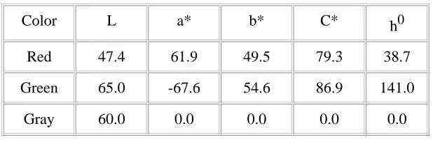
[image:9.612.152.461.197.299.2]Suprathreshold tolerances were measured around 3 color centers in three directions The three color centers are shown in the following table (TABLE I).
Table I. The CIELAB values of the three color centers studied.
Color L a* b* C* h0
Red 47.4 61.9 49.5 79.3 38.7
Green 65.0 -67.6 54.6 86.9 141.0
Gray 60.0 0.0 0.0 0.0 0.0
Each color center was varied in L*, C*, and H* in steps of .3Δ E*ab. For each color center the Δ L*, Δ C*ab, and Δ H*ab values were calculated for every possible pair. From this list 10 sample pairs were selected so that Δ L* varied in step of .3Δ E*ab, 10 sample pairs were selected so that Δ C* varied in step of .3Δ E*ab and 10 sample pairs were selected so that Δ H* varied in step of .3Δ E*ab. The tables in appendix A show the L*, a*, b* values for each color center, color difference pair in each direction.
In each case color pairs were selected so that the total color difference were at least 95% in the desired direction. The range for the sample pairs started at .3Δ E*ab and extended to 3.0Δ E*ab. Therefore there were 30 sample pairs for each color center. In total 70 sample pairs were generated. The same sets of sample pairs were used in both experiments. During the preliminary testing phase of the experiment it became apparent that the thresholds for the green color center were two small. For these cases, additional sample pairs were generated and added to the upper end of the range and sample pairs were removed from the lower end.
Monitor Calibration:
This research project utilized a Sony Trinitron Multiscan 15sf monitor that had been modified by Sony to increase the peak luminance value. The luminance level had been increased to achieve higher absolute light levels for the
experiments. To ensure that the values measured from the monitor are accurate we had to calibrate the monitor.
Calibration refers to achieving a predefined set-up for a display system. Characterization is always required in order to define color in a device-independent fashion.
Calibration was accomplished using the LMT C-1200 colorimeter and the LMT luminance meter in order to measure the colorimetry values of the monitor.
Computer-controlled CRT displays can be described by a two-stage model. The first stage is nonlinear and relates digital counts with the photometric scalars for each channel. The second stage consists of a linear transformation matrix, which relates photometric scalars of each channel with tristimulus values. The first step in the calibration process was to linearize the monitor. Once the monitor was linearized and RGB values were determined it was possible to determine XYZ values and from the XYZ values we determined the CIELAB values. CIELAB values were
E’s knowing the output CIELAB values we were able to specify on the monitor exactly what RGB values to display so that the samples displayed by the monitor varied by .3Δ E*ab. These target values were used to generate stimuli but the actual measured values of the stimuli were used in the analysis.
The calibration process used in this research is identical to that used by Berns et al3.
Experiment:
Visual assessments took place over a 2-week period. 30 color normal subjects ages 19 to 49 took part in the experiment. The subject pool consisted of 5 females and 25 males each with varying degrees of experience in judgin color differences.
The experiment was conducted in a darkened room. Observers adapted for one minute to the background display before beginning the session. The adaptation screen consisted of a neutral gray background with L*=50. This background is used in both MCS and GSC experiments.
To insure that results were not based on which experiment was presented first the order of presentation of experimen was randomized.
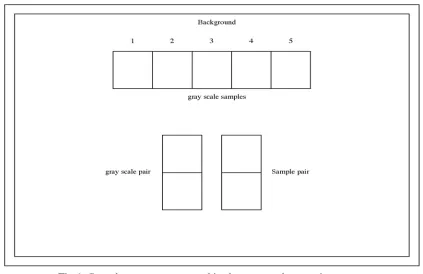
Gray Scale Comparison
The gray scale comparison method used for visual assessment is similar to that used by Luo and Rigg7.
[image:10.612.96.519.357.631.2]The patches in this experiment were 4cm x 4cm. The patches subtended a visual angle of approximately 4.4o when viewed at a normal viewing distance of about 52 cm.
Table IX. The colorimetric values for the GSC display
Object L* a* b*
Background 50.0 0 0
Standard 40.0 0 0
Patch 1 40.5 0 0
Patch 2 41.0 0 0
Patch 3 41.5 0 0
Patch 4 42.0 0 0
Patch 5 42.5 0 0
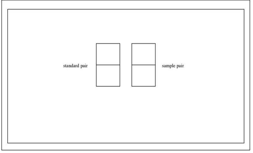
Method of Constant Stimuli:
The method of constant stimuli was similar to that used by Berns et alnumber. In this experiment samples were arranged vertically with a 1 pixel black line separating the samples in the standard pair, and the sample pair. The samples arranged as shown in Fig. 2. The anchor pair was always presented on the left side of the display however; the top bottom position of the anchor pair was randomized for each trial. The trials for the three-color centers were intermixe and presented in a different random order for each observer. The randomization of stimuli is intended to minim sequential effects; it has been shown that observers are incapable of ignoring their previous responses. Obser free-viewed the samples at normal viewing distance for a CRT display. A white border (close to D65) surrounded display defining the reference white. The anchor pair, consisting of two uniform patches, had a Δ E*ab=1.0. The colorimetric values of the display are shown in Table X. Each observer was asked to judge which pair exhibits a lar
color difference by comparing a sample pair and the standard pair5.
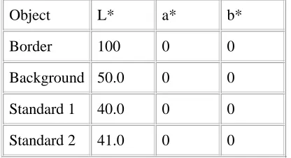
[image:11.612.107.511.428.672.2]Patches in this experiment were also 4cm x 4cm and subtended a visual angle of approximately 4.4o when viewed at a normal viewing distance of 52cm.
Object L* a* b*
Border 100 0 0
Background 50.0 0 0
Standard 1 40.0 0 0
[image:12.612.203.411.23.136.2]Standard 2 41.0 0 0
TABLE XI. Summary of experimental conditions for each experiment.
Psychophysical Method Viewing Background Gap No. of Pairs No. of observers No. of assessments
Gray Scale Gray Hairline 70 30 2100
Constant Stimuli
Gray Hairline 70 30 2100
Results
As mentioned earlier, a panel of 30 observers assessed each pair. For both the gray scale comparison and the method of constant stimuli each observer assessed each pair once.
Method of Constant Stimuli:
The method of constant stimuli data were analyzed using probit analysis, a univariate statistical method that locates a median threshold from binary choice (in this case greater then/less then) visual data. Probit analysis employs the hypothesis that frequency-of -rejection data follow a cumulative -normal distribution. The chi-squared test is used to test this hypothesis. Probit analysis tolerance thresholds corresponding to the pair difference will be determined for each color center and color difference direction. An overall fit of the data will be assessed by a chi-square test. The T50 (50% tolerance level) corresponds to the median color tolerance. The precision of the tolerances is evaluated by the associated fiducial limits. Conceptually, fiducial limits are equivalent to standard error multiplied by 2, because 95% is twice the standard error.
Probit analysis is available through the math program SAS. SAS is available on the Rochester Institute of Technologies VAX computing system. The following figures illustrate the probit fit, the associated fiducial limits and the raw data.
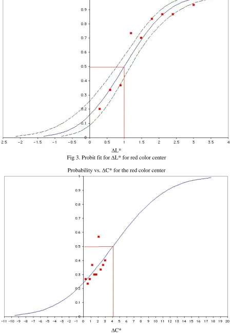
ΔL*
Fig 3. Probit fit for ΔL* for red color center
Probability vs. ΔC* for the red color center
[image:13.612.79.533.34.683.2]ΔC*
Fig 4. Probit fit for ΔC* for red color center
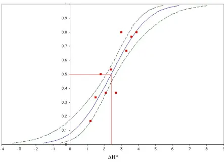
ΔH*
Fig 5. Probit fit for ΔH* for red color center
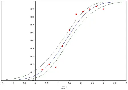
Probability vs. ΔL* for the green color center
ΔL*
Fig 6. Probit fit for ΔL* for green color center
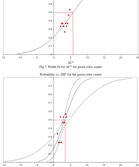
[image:14.612.76.531.38.683.2]ΔC*
Fig 7. Probit fit for ΔC* for green color center
Probability vs. ΔH* for the green color center
[image:15.612.75.529.123.668.2]ΔH*
Fig 8. Probit fit for ΔH* for green color center
ΔL*
Fig 9. Probit fit for ΔL* for gray color center
Grayscale Comparison Method:
For the experiment conducted using the gray scale comparison method, the raw data in Grade (G) units were transformed to the visual difference for each pair Δ V, using the following Eq. 1
Δ V=.1390+.3748*G+.0552*G2-.0052*G3 (1)
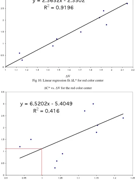
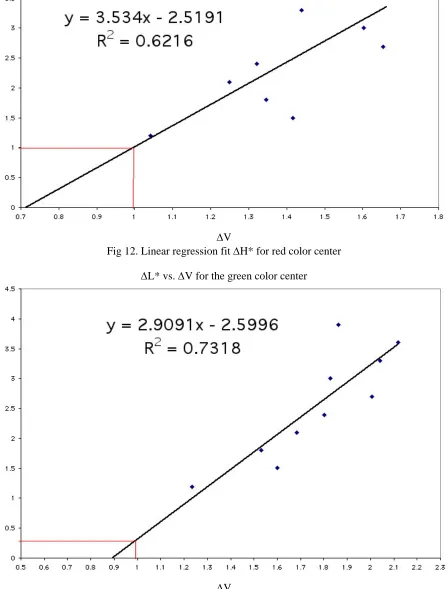
The coefficients in Eq. 1 were obtained by fitting a third-order polynomial equation between the Δ E and grade values. Using Eq. 1, Δ V values were calculated for each observer. The Δ V values were summed across all observers then divided by 30 (number of observers) to obtain an average Δ V value for each sample pair. The corresponding color direction values for each sample pair (L*, C*, H*) were plotted versus the average Δ V value obtained for that particular color difference pair. A linear regression line was fitted to the data and an r2 value was calculated. The r2 value was calculated to assess the fit of the linear regression to the data points. Threshold values were determined by finding the color difference Δ L*, Δ C* or Δ H* which corresponds to a visual difference of 1Δ V.
ΔV
Fig 10. Linear regression fit ΔL* for red color center
ΔC* vs. ΔV for the red color center
[image:17.612.83.526.78.667.2]ΔV
Fig 11. Linear regression fit ΔC* for red color center
ΔV
Fig 12. Linear regression fit ΔH* for red color center
ΔL* vs. ΔV for the green color center
[image:18.612.82.530.90.679.2]ΔV
Fig 13. Linear regression fit ΔL* for green color center
ΔV
Fig 14. Linear regression fit ΔC* for green color center
ΔH* vs. ΔV for the green color center
[image:19.612.82.526.143.663.2]ΔV
Fig 15. Linear regression fit ΔH* for green color center
ΔV
Fig 16. Linear regression fit ΔL* for gray color center
Method Comparison:
The results were used to investigate the differences between the method of constant stimuli and the gray scale
comparison. The visual results from the psychophysical methods are presented in different forms: visual difference (Δ VGS) and visual probability (P) for the gray scale comparison and method of constant stimuli respectively. (The visual probability is the percentage of the number of observations judging the sample pair having a larger difference than that of the standard pair.). To compare the results from each experiment the Δ V threshold values from the gray scale comparison and the corresponding color direction threshold values from the method of constant stimuli were plotted versus color direction. Also plotted are the normalized data points from the gray scale comparison. Normalization of the data were done by finding the mean of the MCS data and adding that mean to the raw data from the GSC. Now the MCS and GSC results have the same mean value.
Color Direction Fig 17. Method Comparison
Discussion
Method of Constant Stimuli
The data from the method of constant stimuli were analyzed using a statistical method of probit analysis. The results are plotted in Fig.1 through Fig. 8. Each of the graphs shows the probit fit to the raw data, the raw data and the
[image:21.612.72.562.48.352.2]associated fiducial limits. Because the chi-square value was small (p>0.1000) the fiducial limits were calculated using a t value of 1.96. All of the raw data from the MCS experiment fit the probit model with 95% accuracy. Using the 50% probability (the point were 50% judged the color difference greater then the standard and 50% of the observers judged the color difference less then the standard) to determine the threshold. The experimental threshold values for each color center in each direction are given in the Table XII.
Table XII. Threshold values from the MCS
Color Direction
Red Green Gray
Δ L*
1.00 1.227 1.325
Δ C*
4.090 5.787
Δ H*
2.405 3.331
Since the probit model fit the data with 95% accuracy the relative accuracy of the threshold values is also believed to be very good.
The data from the gray scale comparison were analyzed by calculating Δ V values using Eq 1. for each observer and calculating an average Δ
V value for each color center in each direction across all 30 observers. A linear regression was fit to the data and the r2
value was calculated. Low r2 values show that the raw data does not follow a linear regression very well.
[image:22.612.204.406.153.284.2] [image:22.612.204.406.402.531.2]The experimental threshold values for each color center in each direction obtained from the gray scale experiment are given in Table XIII.
Table XIII. Threshold values from the GSC
Color Direction
Red Green Gray
Δ L*
0.015 0.310 0.752
Δ C*
1.115 2.034
Δ H*
1.015 0.189
Method Comparison:
[image:22.612.132.477.629.709.2]The MCS was compared with the GSC by comparing the suprathreshold color tolerances determined from each experiment. 50% probability point in the MCS was compared with the 1Δ V value from the GSC. In addition the GSC data was normalized by adding a constant factor so that the new data that had the same average value as the data from the MCS experiment (Table XIII). No consistent trends were seen in the difference between the 2 sets of results.
Table XIII. Normalized threshold values from the GSC
Color Direction
Red Green Gray
Δ L*
1.977 2.272 2.714
Δ C*
3.077 3.996
Δ H*
2.977 2.151
An overall mean and standard deviation was calculated by taking the color difference values from the normalized GSC data and the MCS data. The difference was calculated for each color direction in each direction. The mean was
calculated by taking the average of these differences. This resulted in a overall difference between the two experiments of 1.14 Δ E*ab and a standard deviation of 0.38. The data is shown in Table XIV.
Table XIV. Mean and standard deviation between the experiments.
Δ L* Red
Δ C* Red
Δ H* Red
Δ L* Green
Δ C* Green
Δ H* Green
Δ L* Gray
Average
StdDev
0.98 1.01 0.57 1.04 1.79 1.18 1.39 1.14
0.38
correlation coefficient suggests that there is little correlation between the results of the two methods. The differences may in part explain the differing results obtained from other color laboratories. More data may have yielded the nature of the differences, the determination of the differences between the two methods was out of the scope of this
experiment.
Conclusion
The results support the research hypothesis that differences do exist between the MCS and the GSC methods for deriving suprathreshold color tolerances. There is not sufficient data to see any major trends that may explain the cause of these differences or how these differences could lead to differences in the derivation of color difference formulae. However, the research shows that the differences between the results of the two methods are due solely to differences between the two psychophysical techniques since the same stimuli were presented in each experiment. These
differences may impart explain the discrepancies found between laboratories employing the different techniques.
Based on the results the MCS was determined to be a better metric for deriving suprathreshold color tolerances. The determination of this conclusion is based on the following factors.
First, the method of constant stimuli was easier to implement in code. Matlab provides a relatively easy environment for implementing psychophysical experiments, due impart to the psychophysical toolbox which can be downloaded for free of the internet. The amount of programming for this experiment was far less then that of the GSC method. The MCS employed 300 lines of code while the GSC employed the use of 400 lines of code. Ease of programming allows for a faster cycle time from start to finish. Actual code can be viewed in Appendix: A of this report.
Second, according to the subjects participating in the experiment, the MCS was the easier of the two experiments to perform. The main reasons for this statement were based on overall time to complete the experiment and relative ease of decision making involved. The average time to complete MCS portion of the experiment was 7-10 minutes. The average time to complete the GSC portion of the experiment was 10-15 minutes.
Last and most importantly, the results obtained from the MCS were the more precise. Probit analysis provides 95% confidence intervals for each of the color centers in each direction. The results from the GSC method were far less
accurate. Fitting a linear regression to the GSC provided average r2 values of less then .70.
Given the ease of implementation, precision and reliability of the results the MCS method is the clear choice for deriving suprathreshold color tolerances.
Color Tolerance Comparison
David C. Wilbur
References
Qiao Y, Berns RS, Reniff L, Montag E. Visual determination of hue suprathreshold color difference tolerances. Color Res Appl 1998:23:302-313
1.
Montag ED, Berns RS. Visual determination of hue suprathreshold color-difference tolerances using CRT-generated stimuli. Color Res Appl 1999:24:164-176
2.
Berns RS. Methods for characterizing CRT displays. Displays 1996:16:173-182 3.
Guan, Luo MR. Investigation of parametric effects using small colour differences. Color Res Appl 1999:24:331:343
4.
Berns RS, "Munsell color science laboratory industrial color difference consortium - current initiatives and future directions", Proceedings of the SPE 57th annual technical conference and exhibits, 2873-2877 (1999)
5.
Montag E, Berns RS. Lightness dependencies and the effect of texture on suprathreshold lightness tolerances. 6.
Luo MR, Rigg B. Chromaticity-discrimination ellipses for surface colours. Color Res Appl 1986:11:25-42 7.
Color Tolerance: A comparison of the method of constant stimuli and
gray scale comparison method on a CRT.
David C. Wilbur
Appendix A
[image:25.612.41.381.189.571.2] [image:25.612.43.380.606.714.2]Tables of Colorimetric Values
Table II. The colorimetric values for the red samples varying in L*
Sample Pairs
L* a* b* Δ E*ab
1 46.9313 47.2299 62.5628 62.5595 48.2831 48.3457 .2973
2 47.9352 48.532 62.726 62.7694 48.4598 48.425 .5968
3 46.7563 47.6539 62.5161 62.7272 48.3826 48.4383 .8976
4 46.9313 48.1301 62.5628 62.7412 48.2831 48.5265 1.1988
5 47.1271 48.6201 62.5651 62.7491 48.3654 48.5768 1.4930
6 46.9313 48.7285 62.5628 62.7492 48.2831 48.4774 1.7972
7 45.9169 48.0196 62.3042 62.7427 48.2029 48.5784 2.1027
8 47.6539 50.052 62.7272 62.9489 48.4383 48.6294 2.3982
9 46.4753 49.174 62.4934 62.9172 48.3634 48.5281 2.6986
10 46.6684 49.6736 62.4846 62.9179 48.2599 48.6384 3.0052
Table III. The colorimetric values for the red samples varying in C*
Sample Pairs
L* a* b* Δ E*ab
1 47.5364 47.5791 62.5284 62.7772 48.044 48.2271 .3088
3 47.4774 47.5952 62.2515 62.9962 47.8879 48.3921 .8977
4 47.4882 47.5952 62.0441 62.9962 47.6621 48.3921 1.1998
5 47.515 47.5738 61.8641 63.0563 47.4659 48.3827 1.5040
6 47.4614 47.6272 62.3047 63.7196 47.8601 48.9747 1.8010
7 47.5364 47.5791 61.368 63.0653 47.1561 48.392 2.0989
8 47.531 47.6272 61.8272 63.7196 47.4936 48.9747 2.4030
9 47.5096 47.6112 61.4672 63.5498 47.1365 48.8632 2.7034
[image:26.612.41.381.21.278.2]10 47.4721 47.6752 61.4994 63.8149 47.1515 49.0574 2.9972
Table IV The colorimetric values for the red samples varying in H*
Sample Pairs
L* a* b* Δ E*ab
1 47.4506 47.4882 63.1868 62.3663 47.5974 48.484 1.2027
2 47.515 47.531 63.246 62.2139 47.7083 48.8088 1.5016
3 47.4721 47.4935 63.0142 61.8112 47.8242 49.1671 1.7985
4 47.5791 47.531 63.879 62.5033 46.8606 48.447 2.0949
5 47.4935 47.5471 63.3223 61.6611 47.5096 49.2594 2.4006
6 47.4506 47.515 63.0906 61.2337 47.8417 49.8063 2.6920
7 47.5524 47.5364 63.6756 61.7073 47.0514 49.3262 3.0032
8 47.5524 47.5203 63.6756 61.518 47.0514 49.5559 3.3009
9 47.6272 47.5471 64.0534 61.6611 46.5527 49.2594 3.6029
10 47.5952 47.5471 63.7781 61.2086 46.8359 49.7748 3.8967
[image:26.612.42.378.314.688.2]Sample Pairs
L* a* b* Δ E*ab
1 65.0923 66.2867 -66.9132 -67.1195 54.6378 54.6952 1.1944
2 66.1461 67.6547 -67.0199 -67.1156 54.657 54.7384 1.5086
3 65.0002 66.7971 -66.9721 -67.0084 54.6073 54.6611 1.7969
4 64.3764 66.4745 -67.0501 -67.118 54.6309 54.7346 2.0980
5 64.3764 66.7719 -67.0501 -67.0946 54.6309 54.7242 2.3955
6 64.4299 67.1329 -66.8853 -67.0994 54.533 54.7504 2.7030
7 64.4299 67.4381 -66.8853 -67.1134 54.533 54.7274 3.0082
8 64.6597 67.9623 -66.9499 -67.1803 54.5806 54.7942 3.3026
9 64.0542 67.6547 -66.9945 -67.1156 54.5764 54.7384 3.6005
[image:27.612.43.384.16.387.2]10 63.865 67.7688 -66.9805 -67.1015 54.5328 54.755 3.9038
Table VI. The colorimetric values for the green samples varying in C*
Sample Pairs
L* a* b* Δ E*ab
1 65.7569 65.8215 65.8215 -67.8213 53.9178 55.2173 2.1069
2 65.786 65.8215 65.8215 -67.8437 53.7234 55.2173 2.4088
3 65.8215 65.815 65.815 -68.0625 53.7439 55.3325 2.7082
4 65.786 65.7957 65.7957 -68.3386 53.7234 55.5527 3.0044
5 65.7246 65.8054 65.8054 -68.2679 53.4822 55.4565 3.2978
6 65.7504 65.9117 65.9117 -68.8839 53.8114 56.0222 3.5979
8 65.8054 65.9085 65.9085 -68.6451 53.2716 55.8038 4.2031
9 65.7795 65.886 65.886 -68.9305 53.4151 56.0062 4.5023
[image:28.612.42.384.22.118.2] [image:28.612.42.385.157.520.2]10 65.8279 65.886 65.886 -68.9305 53.0833 56.0062 4.8033
Table VII. The colorimetric values for the green samples varying in H*
Sample Pairs
L* a* b* Δ E*ab
1 65.6793 65.7731 -66.5156 -67.4111 54.9162 54.0959 1.2015
2 65.7537 65.7634 -66.4134 -67.4812 55.1425 54.0792 1.4989
3 65.7569 65.7731 -66.1387 -67.344 55.5566 54.2054 1.8092
4 65.7666 65.8473 -66.1583 -67.6193 55.4461 53.9376 2.0926
5 65.7666 65.8183 -66.1583 -67.8074 55.4461 53.6843 2.4075
6 65.7989 65.815 -66.0095 -67.8607 55.6573 53.6787 2.7999
7 65.7569 65.7892 -66.3829 -68.3558 55.2323 52.9632 3.0045
8 65.7795 65.815 -65.926 -68.0625 55.8227 53.3151 3.2936
9 65.7989 65.8086 -65.8104 -68.2144 55.8561 53.1834 3.5903
10 65.7924 65.8634 -65.9595 -68.5406 55.7597 52.8388 3.8940
Table VIII. The colorimetric values for the gray samples varying in L*
Sample Pairs
L* a* b* Δ E*ab
1 60.3126 60.6082 -0.0987 -0.1336 0.2295 0.1967 .2956
2 60.7331 61.341 -0.1391 -0.2014 0.1988 0.2018 .6078
3 60.4459 61.341 -0.1027 -0.2014 0.2203 0.2018 .8951
5 59.7295 61.2288 -0.1605 -0.1937 0.2436 0.2127 1.4993
6 58.9571 60.7515 0.0138 -0.0852 0.1577 0.0354 1.7944
7 59.122 61.2288 -0.1063 -0.1937 0.2317 0.2127 2.1068
8 59.0531 61.4455 0.0695 -0.129 0.1128 0.1844 2.3925
9 59.122 61.8183 -0.1063 -0.1921 0.2317 0.1684 2.6963
10 58.9571 61.9501 0.0138 -0.1788 0.1577 0.1716 2.9930