Some problems in the theory and application of the methods of numerical taxonomy

SOME PROBLEMS IN THE THEORY AND

APPLICATION OF THE METHODS OF NUMERICAL

TAXONONMY

David Wishart

A Thesis Submitted for the Degree of PhD

at the

University of St Andrews

1970

Full metadata for this item is available in

St Andrews Research Repository

at:

http://research-repository.st-andrews.ac.uk/

Please use this identifier to cite or link to this item:

http://hdl.handle.net/10023/10121

SOME PROBLEMS IN THE THEORY AND APPLICATION OP THE METHODS OP

NUMERICAL TAXONOMY by

DAVID WISHART, B.Sc. ABSTRACT

Several of the methods of nimerioal taxonomy are compared and shown to be variants of a tripartite grouping procedure associated with a generalised intercluster similarity function involving ten computational parameters. Clustering by the tech­ niques of hierarchic fusion^ monothetic division and iterative relocation is obtained using different arithmetic combinations of the function parameters to both compute similarities and effect changes in cluster membership. The combinatorial solution for

Ward’s method is founds and the centroid sorting combinatorial N solution is extended for size difference, shape difference, dis­

persion and dot product coefficients.

ProQuest Number: 10166976

All rights reserved

INFORMATION TO ALL USERS

The quality of this reproduction is dependent upon the quality of the copy submitted.

In the unlikely event that the author did not send a com plete manuscript and there are missing pages, these will be noted. Also, if material had to be removed,

a note will indicate the deletion.

uest

ProQuest 10166976

Published by ProQuest LLO (2017). Copyright of the Dissertation is held by the Author.

All rights reserved.

This work is protected against unauthorized copying under Title 17, United States C ode Microform Edition © ProQuest LLO.

ProQuest LLO.

789 East Eisenhower Parkway P.Q. Box 1346

\

A method for mode-seeking is developed from this probabilistic model through various theoretical and experimental phases, and it is shown to perform slightly better than iterative relocation with the minimum-variance criteria using several Gaussian test popu-• lations.

A fast algorithm is proposed for the solution of the

Jardine-Sibson method for generating overlapping classes, and it is observed that this technique finds natural classes and is closely related to the probabilistic model.

SOME PROBLEMS IN THE THEORY AND

APPLICATION OP THE METHODS OP

NUMERICAL TAXONOMY

by

DAVID WISHART, B.Sc

Dissertation submitted for the degree of Doctor of Philosophy of the

University of St. Andrews.

PREFACE

In October 19^1, I matriculated at the University of St. Andrews and read for a degree in Mathematics at St. Salvator's College, graduating in June 1965 with the

Ordinary Degree of Bachelor of Science. Following my appointment in January I966 as computer programmer at

the Computing Laboratory, I matriculated for the degree of Master of Science in Computational Science. In March I9G9, I was admitted as a candidate for the degree of

Doctor of Philosophy under Resolution of the University Court, 1967, No. 1, and credited with the time spent

towards the M.Sc. degree. Throughout the period 196 6-7 0

DECLARATION

I declare that the following thesis is a record of research work carried out by me, that'the thesis is my own composition, and that

it has not been presented in application for a higher degree previously.

CERTIFICATE

I certify that David Wishart has

satisfied the conditions of the Ordinance and Regulations and is thus qualified to submit the

accompanying thesis in application for the degree of Doctor of Philosophy,

ACKNOWLEDGEMENTS

I am deeply indebted to my supervisor Professor A. J. Cole for his sustained guidance and criticism throughout this work. My thanks are due to everyone who has contributed towards ray experience with the methods of numerical taxonomy through their comments on and evaluation of results. In this respect, I am particularly grateful to Dr. R, M. M. Crawford of the Department of Botany, University of St. Andrews,

for our fruitful collaboration in the studies in plant ecology. I also acknowledge the contributions of Professor D. C. D, Pocock of Erindale College, University of Toronto, and Dr. A. H. Dawson of

CONTENTS

INTRODUCTION •• »• «. •. «» •» » * 1

CHAPTER 1 ; DATA OPERATIONS AND MEASURES OF SIMILARITY 4 1 .1 BASIC DATA CONSIDERATIONS .. .. .. .. 4 1 .2 TRANSFORMATIONS AND WEIGHTING SCHEMES . . . . l4 1.3 PRINCIPAL COMPONENTS ANALYSIS .. ., .. 25

1.4 SIMILARITY COEFFICIENTS . , 39

CHAPTER 2; HIERARCHIC FUSION . 2.1 GENERAL PROCESS

2.2 METHODS 2.3 DISCUSSION

CHAPTER 3: DIVISIVE METHODS . . 3.1 MONOTHETIC DIVISION . 3.2 POLYTHETIC DIVISION .

CHAPTER 4: ITERATIVE RELOCATION 4.1 GENERAL PROCESS

4.2 METHODS 4.3 DISCUSSION

51 51 54 66

72 72 87

96

96

99 109

CHAPTER 5: GENERALISED TRIPARTITE PROCEDURE

5.1 INTERCLUSTER SIMILARITY FUNCTION 5 .2 METHODS ...

5 . 3 DISCUSSION

113 113

CONTENTS

CHAPTER 6; THE PROBABILISTIC MODEL

6.1 MINIMUM-VARIANCE TECHNIQUES . 6.2 NATURAL-CLASS METHODS

6.3 SINGLE-LEVEL MODE ANALYSIS 6.4 HIERARCHICAL METHOD

6.5 DENSITY FUNCTION AND LARGE POPULATIONS 6.6 AVERAGE DISTANCE AS DENSITY ESTIMATE ■ 6.7 IMPROVED ALGORITHM...

CHAPTER 7: EXPERIMENTAL TESTS

7.1 ITERATIVE RELOCATION TESTS 7.2 HIERARCHICAL MODE ANALYSIS

7 .3 CONCLUSIONS ..

CHAPTER 8; COMBINATORIAL COEFFICIENTS ,. 8.1 LANCE-WILLIAMS ’ 4-PARAMETER MODEL 8.2 WARD'S METHOD .

8 .3 CENTROID SORTING

8.4 COMBINATORIAL ALGORITHM

CHAPTER 9: _{K-PARTITION .}

9.1 JARDINE-SIBSON ALGORITHM 9 .2 COLE-WISHART ALGORITHM . 9 .3 CLUSTER RECOGNITION ALGORITHM

9.4

CHAPTER 10; COMPUTER TECHNIQUES

10.1 TOWARDS GENERALISED STATISTICAL SYSTEMS 10.2 DATA STORAGE AND RETRIEVAL TECHNIQUES . 10.3 FEATURES OF CLUSTAN ...

CONTENTS

CONCLUSIONS .. . . . . . . ., , , ». . . .. 255

BIBLIOGRAPHY ... . , . . . . . . . , 259

APPENDIX I; APPLICATIONS . .. .. .. ,. .. .. 268 la PLANT ECOLOGY... . . . , . 268

Ib URBAN REGIONALISATION ». 342

Ic CLASSIFICATION OF DISEASES .. .. ». .. 368

Id MAPPING AREAL GEOLOGY ... . . . . 378

le PLATONIC PROSE RHYTHM AND CHRONOLOGY .» ., 386

APPENDIX II; .SUBROUTINE DISKIQ ’... ..421

- 1

-INTRODÏÏCTION

Numerical taxonomy could be described as the branch of multi­ variate statistics which is concerned with the simplification and description of observational data. Two general problems arise in

connection with data simplification. Firstly, an observer who wishes to describe statistically a 'concept' or 'frame of

reference’ which he has chosen for study may encounter difficulty in the selection of relevant variables. Secondly, methods of analysis must be found which fit both the types of data and the way in which they are to be treated. Selection of variables which characterise a complex concept, such as ’areal class structure of a town’' or ’hominoids', depends largely on the observer’s personal idea of which measurable attributes contribute usefully towards the variability within his sampling frame. At this stage, considerations of methodology should not arise, for the observer must be completely free to make any measurements which he thinks

are important. The statistician must therefore design methods which take into account all aspects of sampling, making allowances for such undesirable effects as strong multiple correlations, the inclusion of poor variables, weak orthogonal components, and so on. It is very easy to sidestep the consideration of data and

One of the least studied aspects of the subject is structure in the multivariate sample space, and there is sometimes a very dangerous tendency to dismiss this topic altogether - I refer to writers who begin tidily with "a suitable similarity matrix” and proceed to define rigorous procedures based on intuitive ideas of what should be done with similarity coefficients. Another hazard is the 'logic' deduced from descriptive arguments which use the M-dimensional euclidean space as a model, 'thinking' of it in

terms of ^-dimensional reality. Who is to say that M-space

behaves like 1, 2 or 3~space? There are some excellent examples of the unpredictability of M dimensions (Day, 19T0)o On the other hand, we cannot afford to be so confident as to reject altogether the euclidean model as an indicatorj yet there are those who adopt a more topological approach to the subject, and appear to regard the euclidean model as a rather trivial specia­ lisation (e.g. Jardine, et al, 1967).

One source of information that we cannot possibly ignore is the wealth of empirical evidence which appears throughout the literature in the justification of individual procedures. It was surely empirical studies which revealed the chaining effect of single linkage and fragmentation in association

-3-Investigation which are most likely to lead to a formal theory. Consequently, an important part of the work reported here has been the development of a system of computer programs for cluster analysis which is available to workers in all disciplines for the collective empirical study of existing methods. The system has been carefully designed to make it easy for new procedures to be added - indeed, despite the rather complex use of magnetic disk and tape (Chapter 10), the actual clustering programs are totally machine independent; thus a new procedure can now be introduced at about 50 installations throughout the world with­ out any changes in data set assignments or the job control language specifications for each machine and operating system.

This thesis is concerned more with the treatment of data and the properties of methods, An attempt has been made to survey the range of methods, making generalisations where

possible in order to deduce their common properties. In a sense, the work constitutes a classification of classification methods using as data the kernel of each technique considered. Every

CHAPTER 1 : DATA OPERATIONS AND MEASURES OP SIMILARITY 1.1 BASIC DATA CONSIDERATIONS

The general objective of cluster analysis is to find a grouping of N individuals into k classes which is 'meaningful', and constitutes a useful classification of the population. This very vague statement is about as near as we ever get to genera­ lising the methods of numerical classification. In order to be more specific we must divise numerical models to represent popu­ lations, specify structural limits for the k classes, interpret the notion 'meaningful' in relation to actual problems or abstract generalisations, and explain how the results can be used. We can, however, state the general classification result as follows: 1. There shall be k groups of individuals such that each

group contains at least one individual,

2, Each individual may be assigned to no group (if it is 'unclassifiable'), one group only (if disjoint clusters are required), or more than one group (when overlapping clusters are permitted),

-5-“ Continuous data

’Continuous' or 'quantitative * data are measurements of quantities which range on a 'continuous' scale. We can easily distinguish between quantitative and qualitative (see below) observations, but it is sometimes less easy to say when a con­ tinuous variable can no longer be treated as such, and should be regarded as an ordered multistate character (see below). For example, we may regard population in countries as continuous

(the range is 'continuous' on a scale from a few thousand to

600 million); similarly, population in cities and towns, boroughs,

or wards may be treated as continuous; however, is it reasonable to treat population in houses or rooms of houses as a continuous variable, when the range is only about 1 to 10? Thus we have encountered the first demand for subjective decision, namely, the choice between the treatment of semi-quantitative data as either continuous or multistate variables.

A typical small raw continuous data matrix is shown in Table 1.1,1. Six variables (the number of service establishments per 1000 population for six categories) are measured for nine

individuals (census divisions of the USA). We denote by the value of variable j for the ith individual (the jth element of row i in Table 1 .1 ,1 ), and define the mean and variance for

variable j by ^

-6-I—I

VO CO OV 00 00

-P -P

Q) P>

VO VO OJ LfA (— m LA

o OV OJ 00 -=^- lA

VO i>- VO 00 in 00 00 00 00

m ^ OJ

in LA in OV 00 00m VO 00 \o 00 00

II

LA in in t—

h-OJ ^ LA 00

Ô Ô o Ô 00

LA in

I—I

g 00_tn 0000

CO

I— 1 I— I

CO

"7”

P 1 M p

variance S = - 21 (X-1 " Uj (1 .1 .2)

J _{JlfS I}4,' 1 J

where N is the number of individuals^ and M the number of variables. The standard deviation is therefore given by Sj.

Table 1.1.1 also shows the mean, variance, standard deviation, minimum and maximum for each of the six variables; we observe

that the category 'personal' has the largest variance (0.144) and range (I.3 2), while 'amusements' has the smallest variance (0.005)

and range (O.2 5).

Numerical classification techniques are invariably concerned with the comparison of individuals or groups of individuals

(clusters) in terms of the set of M variables. Perhaps the most common measure of the similarity between two individuals is the

'squared euclidean distance' coefficient: each individual is represented by a point in M-dimensional space whose coordinates are the associated M variable scores, and we may compute the

2

squared distance d^^ between two points i and k using the formula

,2 1

J = l

2

Thus, for example, using the data of Table 1.1,1 d^^ is

[(2.5 6-2.7 0)^ + (0.5 7-0.7 2)^ + (0.5 3-0.5 4)^ +

(0.6 9-0.7 2)^ + (0.4>0.4l)^ + (0.46-0.25)^1

-8-2 2

) is the component of which is attributed to

vari-2 2

able j, and the mean of this component for the N possible d^^^ coefficients is

N N

E(d^), =-2 Z IT - \ , f

N i=l k=1

\ _{Z k [(X^J - Ü.) - ()^J - u.)]"}

2

N i k

which reduces, after expansion, to

- p Z n + N (X - U )

N i iJ J

= 2Sj

2

It follows that the expected contribution to d of each variable is proportional to the variance, and hence the distance coefficient is biased towards variables with high variance. From Table 1.1.1, we see that the mean of the distance component for the category

'personal* is 0.288^ while for 'amusements'the mean is 0.01. Variable 1 is therefore weighted by the factor 288, and conse­

quently 'amusements' has almost no influence on the resulting dis­ tance coefficients. For this reason it is customary to 'standardise' continuous data so that the contributions of each variable are of equal importance. This is achieved by replacing each X^j with

X. . = X. ./8. _{I J I J J} (1 .1 .4)_{^ ^}

or, more usually, X. . - U.

-9

-Both standardisations transform the variables to unit variance,

2

so that the expected contribution to d of each variable is 2. (1.1.5) is the more usual formula since the resulting scores have

zero mean; strong deviations from the mean are then easily observed as deviations from zero in the X^^'s. Table 1.1.2 shows the

standard scores obtained using formula (1.1,5) with the data of

2

Table 1.1.1. Since the expected component of d for each vector

2

of standard scores is 2, the expected value of d for M indepen­ dent continuous variables will also be 2; however, this result is of little value since independence can seldom be assumed.

Census

Division Variables

(Sample) 1 2 3 4 ₅ 6

1 _{1 .1 9} 0 .2 5 _{-0.51 -0 .0 9} -0.4o -0 .1 2

2 1.56 1.10 -0.44 0 .1 3 -0 .6 9 -0.84

-0.01 -0 .1 8 _-0 .5 9 —0 » 16 0 .0 3 -0 .6 7

4 0 .0 2 -0 .5 6 0 .8 7 0 .9 8 1 .49 0 .1 2

5 -0 .9 4 -0 .8 8 -0 .8 2 -1 .22 _{-0 .5 5} -0 .2 6

6 -1.88 -1 .63 -1.67 _{-2 .0 7 -1.86 ”0 «} 94

7 —0 .1 6 -0 .4 7 0.64 0 .6 9 -0.11 -0 .3 2

8 -0 .4 7 _{0 .2 3 0 .7 9 0 .5 5} 1 .3 4 2 .5 6

9 0 .7 0 1.97 1.72 1 .1 9 0 .7 6 0 .4 7

Table 1.1.2. Standard scores derived from the data of Table 1.1.1 ing equation (1.1.5)

Binary data

semi-

-10-continuous data, we must adopt the alternative 'qualitative' or 'binary' mode. This enables the recording and manipulation of ' qualities ', of which the most fundamental are binary attributes that can exist in one of two states: present or absent. In fact, we shall see later (Sect, 1.2) that all other qualitative data

can be reasonably transformed into 2-state attributes, so that the binary mode becomes the single alternative to continuous data.

The binary data for N individuals which possess or lack M attributes is usually recorded using an N x M binary matrix such as Table 1.1.3° By convention, 'presence' of an attribute is

Binary attributes

CASES 1 2 3 4 5 6 7 8 9 10

1 1 0 0 1 0 1 0 0 0 ₀

2 0 0 1 0 0 1 1 0 1 1

3 1 0 0 0 1 0 0 0 1 0

4 1 1 0 0 0 1 1 1 1 1

Table 1.1 ,3° A typical binary data matrix for 10 attributes and

4 individuals

-11-having coordinates

^^i 1 ^ ■* ^iJ '* ' ■* ^iM ^

While such data are clearly discrete (the points lie only at the vertices of an M-dimensional hypercube), there appears to be no reason why the intuitive rules of continuous data cannot be equally well applied to binary data using the above spatial representation. In fact, we may evaluate the mean

M

i _{J — '}

J

where p^ is the probability associated with attribute j, and variance (from 1.1 .2)

2 + (N-f.)p^

q _ J <J _________ J J

j N

= Pj(l-Pj) (1.1.6)

and then standardise using equation (1.1.5) so that a.. is re­

placed by a.. - p.

1 (1.1.7)

/ P j ( l - P j )

Standardisation of binary data is not usual, but it has been

suggested by Lance and Williams (1966c) and Williams et al (1 966),

and the latter writers state the following case:

- 12

-common attributes (or Joint absence of two rare ones). To weight such joint occurrences appropriately, the attributes are standardised before the analysis begins," Such arguments can be seen to be dangerous when we extrapolate to an extreme, such as attributes having only 1$ occurrence, Prom

(1,1.6), the attribute variance is

Sj = .01( .99) = .0099

SO that those individuals i which possess such an attribute have

standardised coordinate (1.1.7) of

X , = =. 9,95

7 0 0 9 9

while all other individuals k have coordinate

X^. - 7 = = = -0.1

1 0099

Hence the component of distance is zero in the comparison of a possessing individual i with any other possessing individual 1, or a non-possessing individual k with any other k, while in the comparison of any possessing individual i with a non-possessing individual k the component of distance is

P p

(9 .9 5 - (-0.1)) = (1 0.0 5) = 101

-13-attribute j, to the extent that ordinary data are worthless. Since binary data are already 'normalised', in the sense that the range of values for each attribute is 1, it is probably safer in general to use unstandardised l/O data, thereby avoiding the weighting of rare attributes (see also Sect. 1.2),

Multistate characters

The idea of a binary attribute existing in one of 2 states can be extended to that of a multistate attribute which can exist in one of R states. We shall distinguish between two types :

ordered multistate and unordered multistate characters, which differ according to whether two particular states can be said to be more closely related than two others. An example of an

unordered multistate character is 'colour of hair' - Table 1.2.2. In this instance, we cannot convincingly say that two colours are more closely related than any other two. The converse is an ordered multistate character, for which there is a very definite relationship between the states that must be taken into account. Table 1,2.3 contains the example of 'age' coded as an ordered multistate character. We shall assume that a certain sample popu­ lation of ladies, although unwilling to state their actual ages, were prepared to say whether they were in their 'teens, twenties,

-l4-1 ,2 TRANSFORMATIONS AND WEIGHTING SCHEMES

In the previous section four types of observational measure­ ments were introduced^ together with such fundamental operations as standardisation and the computation of distances. We must now consider ways of transforming data of one type into another type so that unbiased measures of similarity (such as distance) may be evaluated using standard formulae. The four possible data types previously Introduced are:

Continuous Binary

Ordered Multistate Unordered Multistate

but we shall restrict data for analysis to only the continuous

and binary computation modes. The following transformations, which have been discussed by Wishart (I9ô9d), enable any of the four data types to be expressed in either of these two computation modes, and all possible combinations of these transformations are summarized in Table 1,2,5•

_?BC* to Continuous

It has already been suggested that binary data may be treated

as i / o _{M-dimensional coordinate vectors which may or may not be}

standardised. Hence, in order to compare binary and continuous data in the continuous mode we simply code the binary attributes

-15-scores as quasi-contlnuous. This transformation is illustrated, in Table 1.2.1.

Binary Continuous

'present' 1

'absent' 0 TBC>

1. 0

0.0

Table 1.2.1. Transformation from binary data into the continuous computation mode

T,,_,: Unordered multistate to Binary

— UB —'— —— ---

---For an unordered multistate character having R states we create R binary attributes, such that each state is coded as the

'presence' of one attribute. T^^ is illustrated with the 4-state character 'colour of hair' in Table 1.2.2,

Unordered Binary

multistate

White 1

Red 2

Brown 3

Black 4

TUB

1 2 3 4 1 0 0 0 0 1 0 0 0 0 1 0 0 0 0 . 1

Table 1.2.2. Transformation from an unordered multistate character into the binary computation mode

Tqj^: Ordered multistate to Binary

- 16

-such that the jth of these attributes is coded 'present' only for those individuals having a character state code greater than j. This has the effect of introducing a more positive match between

adjacent states than between distant state codes. Table 1.2.3 illustrates T^^ for a 4-state character, and it is seen that, for example, the component of unstandardised distance ranges from 0

(total match) through 1 and 2 to 3 (in the comparison of states 1 and 4).

Ordered Binary

itinuous Zones multistate _{1 2 3}

15 10-20 1 0 0 0

25 _TCO 20-30 2 _'^OB 1 0 0

32 -- — > 30-40 3 ---^ 1 1 0

43 40-50 4 1 • 1 ■ 1

Table 1.2.3* Transformations T^^ and T^^ which convert a con­ tinuous variable to ofdered multistate, and ordered multistate to binary, respectively.

T^Q: Continuous to Ordered multistate

To transform continuous data into the binary computation mode the first step requires the computation of an ordered multi­

-17-a person's -17-age w-17-as in the r-17-ange 10-20, 20-30, 30-40, or 4o-50. Table 1,2,3 shows transformation T^^ for this variable, and it is

seen that T_^ can then be combined with T^_ to complete the trans-_{0Ü üij} formation T«.^ from continuous data to binary,

T ; Ordered multistate to Continuous

This transformation, illustrated In Table 1,2,4, is weakest when generalised. Depending on the relationships between the R states of an ordered multistate character, numeric values are chosen to replace the state codes accordingly. In the example, we replace codes 1,2 and 3 by the same numeric values. The selection of these substitute codes is crucial, even if the resulting vector of scores is standardised, because the dif­ ferences of the codes from the overall mean are reflected propor­ tionately by the standard scores. Every attempt should be made to associate the inserted codes with the means of the ordered intervals which they represent. For example, a percentage variable which has been zoned 0-30, 30-50, 50-70, and 70-100 could have sub­ stitute codes 15;, 40, 6o and 85 if the distribution is known to

be rectangular, or 22, 43, 57 and 78 if it is a normally distri­

-18 -Ordered

multistate Continuous

1 1 .0

2 _Toc^ 2.0

3

....

3.0

Table 1,2.4. Transformation from an ordered multistate character into the continuous computation mode

Table 1.3*5 shows how these five transformations can be com­ bined to convert data of all four types into the two basic compu­ tation modes,

TO

PROM Binary Continuous

Binary — _TBC

Continuous T + T _{CO OB}

Ordered

multistate TOB T00

Unordered

multistate TUB T + T UB BC

-19“ Standardisation

In Sect, 1.1 it was argued that continuous data should be standardised so that each variable has a mean distance component of 2. It was further argued that when binary data are standardised then the distance component of rare binary attributes can bias coef­

ficient values to such an extent that other data are worthless. This complaint can also be applied to continuous data which is

"ill-conditioned", in the sense that some values do not conform to a nicely rounded density function. For example, if we were to count the numbers of theatres in a survey of British towns then almost all the values will be near 1, and not exceeding about 5• By comparison, the count for London would be of the order 50, and the standardised value would probably also be about 50. The squared distance component of a coefficient which compares any other town with London would therefore be of the order 2500, which does not compare at all favourably with the mean 2. We can assume that if a classification problem exists, then the density function for some variables cannot be expected to exhibit nice unimodal dis­ tributions. Standardisation must therefore be used with care, and can dangerously influence the results if applied to ill-con­ ditioned data.

Normalisation

—20” 2

that max(d^^) - 1 . Binary data are treated as variable values 0.0 and 1.0 (transformation T _); continuous data are recorded_Bb as

X. . - mln(X..)

h j "'max(X..) - min{X..) (1.2.1)

where min(X,.) and max(X..) denote the bounds of variable j. Multistate characters are transformed using where the sub­

stitute code for the jth of R states is ( j - i )

(

)

Hence the multistate character codes 1-5 become 0.0, 0.25, 0.5,

0 .7 5 and 1.0 (Parks does not appear to distinguish ordered from

unordered multistate characters).

The great disadvantage of this technique is that the resulting scores are determined by single bound values. In the previous

example of theatres in British towns, the range of values for this variable throughout towns other than London would be either 0 to

5 /5 if London were excluded, or 0 to 5/50 if London were included.

Thus the inclusion of a 'rare' extreme individual is seen to radically influence the coding of the rest of the population (it should be noted that mistakes in the recording or coding of data might have the same effect).

-21

-than the standard deviation as normalising factor with continuous data. If we use Parks' normalisation (1,2.1) instead of standardi­ sation (1.1.5) with the data of Table 1.1.1, then we obtain the

2

standard deviations P . and variances P. which are shown at the_{J J} bottom of Table 1.1.1. Since the component of distance for any

2

variable j has a mean of 2S^, we see immediately that Parks weights variables 4 and 5 more heavily than variable 2 by a factor of 1.24. Also, if we were to add binary data to con­ tinuous using Parks' normalisation, then any binary attribute

having 50^ occurrence has standard deviation (from 1.1.6) S. =0.5

2

and variance =0.25. Thus such an attribute is weighted roughly 3& times heavier than variable 2, and 2-g times heavier than variable 4 of Table 1.1.1. It would seem, therefore, that Parks' normalisation is undesirable when used with mixed-mode data. Weighting Considerations

Table 1,2.5 contains a summary of the proposed transformations from all four variable types into either binary or continuous

data. These transformations do not account for any further

weighting which is designed to standardise or normalise the obser­ vations, and methods must therefore be devised for eliminating or reducing bias. In the case of continuous data, all transformations yield one variable and therefore the origin of the data is not

-22-of each continuous variable regardless -22-of its derivation, provided that account is made for ill-conditioned variables.

With the binary case, the creation of more than one binary variable from a multistate character (which encompasses all three other types) immediately introduces a bias. For any multistate character, let there be R states such that for N individuals the jth state occurs f^ times. We define the probability of the jth state as p. = f./N, and now deduce the mean component of binary distance for multistate characters.

Unordered multistate (T^^).

Table 1.2,2 shows the foUr possible binary patterns obtained from the transformation (T^^) of an unordered 4-state character to binary. The number of times that two individuals will match scores is given by

t(0) = / +

2

and the total number of comparisons between individuals is N , Hence, the frequency of a mismatch, for which the component of binary distance is 2, is given by

t(2) = ^ /

J=1 J

-23

-E(d^) = 2(N^ - H f^)/N^

J=1 R p

- 2(1 - Z P J

J=1 ^ R

= 2 ZT p,(i-pJ

J=1

Ordered multistate (11^)._Uxj

In Table 1.2.3 a continuous variable is transformed by T^ into an ordered multistate character, which is then transformed by T^g into 3 binary attributes. We observe that attribute j is

'present' for all state codes greater than j. In this example, we can write the expected frequencies of each component of binary distance (from 1 to 3) as follows:

t(i) = + fpfj +

t(2) =

t(3) =

The total sum of binary distance components t can now be written as:

t = ^1^2 ^ ^

+ 2(f,f^ + fgf%) + 3(f\f4)

which, in general, is obtained with the formula

-24

-5

A,

As shown In Sect, 1.1, the mean distance component of a continuous 2

variable is 28., which reduces to 2p.(l-p.) in the case of a single _{J J J} unstandardised binary attribute. It would seem, therefore, that an adequate standardisation is obtained if the scores for each type of variable are divided by the appropriate mean distance componentJ in the case of multistate characters, each binary

attribute produced by T or T should be weighted by the overall_{U x j UB} mean distance component. However, this scheme holds only for the manipulation of distances. We should now extend the principle of evaluating mean coefficient contributions to any similarity measure. For example, with the dot product coefficient (Sect.

1.4)

1 M ®ik M J = 1

the mean component of variable j is seen to be

In this case, therefore, it would appear that each variable j is

2

unbiased only when divided by .

-25-problems which exist. In general, we shall assume that an appropri­ ate weighting scheme has been chosen, and the desired transfor­

mations have been completed. The data for classification will therefore take the form of an N x M matrix of either binary pre­ sence/ absence (I/O) scores fa. .J _{i J"*} or continuous variable values

1.3 PRINCIPAL COMPONENTS ANALYSIS

Berry (1961) suggests that a transformation to principal

component scores will eliminate the redundancies incurred when several variables display a single pattern of concomitant vari­ ation. Each pattern of correlated variables is replaced by a single component which represents the pattern, and the point dis­ tribution can be described approximately in terms of a smaller num­ ber of uncorrelated component variables. It is certainly true that, as Berry claims, the transformation will in some instances save

-26

-completely different from those derived, for example, from health variables). It cannot be stressed too strongly that the results obtained from any classification technique are dependent on the original choice of variables, and therefore the derivation of

'meaningful' principal components can be extremely helpful where clarification of the frame of reference is required.

In principal components analysis, the original coordinate axes are rotated to a new set of orthogonal axes so that the major axis (factor) is the line of best fit through the point swarm

(that is, it accounts for the maximum amount of variance), and successive factors are similar lines of best fit subject to the constraint that they must be, in each case, orthogonal to each of their predecessors. The result can be demonstrated by a set of points which lie in a plane through a three-dimensional space. The first axis will lie along the line of best fit, the second

-27-computed on these factors alone, are used for measuring distances, good approximations to the true distances in M-space are achieved. This reduction from M variables to a few (f, say) factors corres­ ponds to a projection of the point swarm from M-space into f-space with the minimum possible distortion of the point orientation,

1

Factor loadings, or eigenvectors, obtained from the product- moment correlation matrix for the six variables of Table 1.1,1 are shown in Table 1.3-1, and the corresponding transformation to factor scores is given in Table 1,3.2,

Variable 1 2 3 4 5 6

Component: 1 _0.31 0.4o 0.47 0.48 0.44 _0.31

2 -0 .6 3 —0. 4l 0.14 -0 .0 6 0 .3 3 0.55

3 -0 .1 6 -0 .4 3 0.31 0 .3 9 0.24 -0 .6 9

4 0 .5 4 -0 .5 0 -0.51 0 .0 9 0.42 o . i4

5 -0.21 0 .4 3 -0 .2 5 -0 .3 9 0,68 -0.31

6 _0.37 -0.24 0 .5 8 -0 .6 7 _0.09 -0.02

Table 1.3-1 - Factor loadings (eigenvectors) obtained by principal components analysis of the USA census data of Table 1.1.1

for a fuller account of the method of evaluating principal com­ ponents analysis see either Cooley and Lohnes (1964), or

)--28

-Census

Division Components

(Sample) 1 2 ₃ 4 ₅ 6

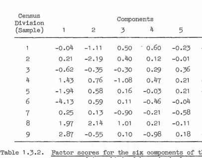
1 - o . o4 -1.11 0.50 ' 0.60 -0 .2 3 -0 .1 2

2 0.21 -2 .1 9 o .4o 0.12 -0.01 0.06

3 —Go 62 _{-0 .3 5} -0 .3 0 0.29 0.36 0.18

4 1 .43 0.76 —1.08 0.47 0.21 -0 .0 7

5 -1 .94 0 .5 8 0.16 _{-0 .0 3} 0.21 -0 .1 6

6 _{-4.13 0 .5 9} 0.11 -0.46 -0.04 _{0 .0 3}

7 0.25 0 .1 3 -0 .9 0 -0.21 -0 .5 8 o .o4

8 _1.97 2.14 1.01 0,21 —0*11 0 .0 8

9 2.87 -0 .5 5 0.10 -0 .9 8 0.1 8 -0 ,0 5

Table 1.3.2. Factor scores for the six components of the USA census data, obtained by principal components analysis

The contributions of components 5 and 6 to the distance coefficient for any two samples may be seen to be small by com­ parison with the four major components. There is little dif­ ference between the distance measures obtained using (a), all six standard scores and (b), the first four component scores. When distances are obtained using all six factor scores (as

adopted by Berry), the results are identical to those derived from the standard scores, and in this instance, the principal components analysis is ineffective.

—29“

space. H. P. Kaiser (1959) suggests a rule for principal components analysis where significant components are those which account for an eigenvalue not less than unity, but whether this rule should be adopted for classification methods is doubtful, for, on the basis of the unity rule, only the first two factors obtained from the present census data would be adopted (Table 1.3*3)° While it is true that combined they account for 88.5 per cent of the overall

Variation Explained

Cumulative Component Total Percentage Percentage

1 3 .9 4 65.7 6 5 .7

2 ₁ .37 2 2 .8 88.5

3 0 .3 9 6 .5 9 5.0

4 0.2 2 3 .6 98.6

5 0.07 1.2 99 .8

6 0.01 0 .2 _100.0

Table 1 .3*3» Analysis of the variance within the USA census data of Table 1.1.1 by principal components analysis

variance, the sizeable contributions to the distance measures of the scores for factors 3 and 4 in Table (1.3-2) suggest that, for classification purposes, the unity rule would involve an over­ simplification and create excessive distortion. However, the

-30

-cannot be selected. The suggestion by D. P. Morrison (196?) that components should be chosen which together explain some arbitrary percentage of the total variance seems to be more pertinent to classification methods, and a level of 90 or 95 per cent of the variance would be reasonable.

More recently. Berry (I9 6 5) has proposed an additional

standardisation of the component scores prior to classification. This effectively destroys all relationship between distance

measures obtained using the original standard scores and the new component scores. The components are standardised in such a way that they have equal importance, a state which is clearly not substantiated by the many applications of principal components analysis. Problems now arise concerning the number of components which should be used, and the incorporation of components which do not have meaningful interpretations. But what is most impor­ tant is that the technique has the effect of creating a 'syn­ thetic' frame of reference in which inter-sample similarities no longer correspond to the observed relationships. Classification methods which derive similarity measures from eigenvectors

normalised in this way produce their results from a frame of

-31

-The adoption by D. M. Ray and Berry (19 6 5) of an additional

rotation from the principal components solution to a normal Vari- max frame of reference has certain advantages concerning the interpretation of factors. This may be adopted when meaningful principal components cannot be derived and a factor analysis appraisal of the data structure is desired. It is not clear, however, whether Ray and Berry use scores computed from Varimax factors for their similarity measures. If this is the case, and' the only axes rotated are those corresponding to the f eigen­ vectors which would otherwise be used to compute distances, then the distances using the f "Varimax factor scores will be the same as those derived from the f major component scores. On the other hand, if more than f axes are rotated to a Varimax solution,

then more dimensions will usually be required to compute accurate distances since the Varimax rotation does not result in an opti­ mal variance solution as obtained by principal components. The effect of Varimax is to share out the large variance explained by the major components among the lesser components in order to obtain factors which lend themselves to easier interpretation. Distances calculated from the major Varimax factors are still good approximations to those obtained using standard scores, but are less accurate than those derived using principal components loadings,

-32

-the number of dimensions used to compute distance coefficients is desired, then factor scores obtained from those eigenvectors associated with the major principal components, which together account for an arbitrary proportion of the overall variance, should be used. A Varimax solution may be obtained as an auxiliary investigation but should not be used in conjunction with classification procedures.

Scatter Diagrams

One of the most useful functions of principal components analysis is that of a diagramatlc tool in the interpretation of cluster structures and relationships. Firstly, we may plot a scatter diagram using any two components as orthogonal axes and their scores as point coordinates (it is customary to plot com­ ponent I against component 11 - the principal plane). Supposing that the population of N individuals has been assigned to k dis­ joint clusters (coded from 1 to k), then instead of plotting stars or crosses on the scatter diagram we may plot cluster codes. Using the principal plane we obtain the best possible 2-dimensional representation of cluster distributions in M-space, and it is often the case that a very large proportion of the overall M-space variance is displayed (see, for example. Appen­ dix le). It is now proposed here that each cluster may be repre­

-33

-joint variance of the cluster distribution. An important

requirement is that the ratio of the lengths of the axes should be equal to the ratio of the latent roots. If this is

not the case, then the displayed interpoint distances will not correspond to the actual distances in space. Thus, for any two

2 2

components x and y having variances S and S we require that_{X y} u - 8 where u^ and u^ are the lengths of the axes.

The circle for cluster t will therefore be centred on the mean (x^,y^) where

2 2

and have radius iS _^ + S ^ where_{xt yt}

is the variance of component x for the subset of individuals belonging to cluster t. Examples can be found in Figure 1,3.2 and Appendices la and le.

Molecular Models

The above technique may be extended for the representation of cluster distributions in the principal 3-space. Each cluster is designated by a sphere having centres (x^,ÿ^,z^) and radius

2 2 ~

^xt ^yt ^zt y and z are the first three principal

]

—34'“

which can then be photographed from different angles (e.g. Boyce,

1969)» Alternatively, we may use a computer program to plot

different views of the molecular-type cluster structure: such a program has been written at St. Andrews by P. G. Adamson in Assembler code for the IWi 1620 (Cole and Adamson, 1969), and is

currently being translated into Fortran IV for the IBM 360 series.

Rotating Principal 3-Space

The following method enables a 3-diraensional distribution to be orthogonally projected on to any 2-dlmensional plane defined by its normal, and can therefore be used to plot cross-sectional scatter diagrams of principal 3-space (or any other space),

A plane is defined by a normal VC, where V(v ,v ,v ) is_{X y z}

the viewpoint and C(c__,c__,c_) _{X y z} the centre of vision. Let (x.,y.,z.)_{1 i i} be the coordinates of the ith point in the principal 3~space, then we can transform the origin to V and rotate the axes so that VC coincides with the new Z axis. If we now compute the coordinates (Xi,Yi,Zi) of the ith point with reference to the new axes, then (Xf,Yi) are the point's coordinates in the plane which is ortho­ gonal to VC. It is easy to show (Cole, I9 6 6) that

'x.'₁

Y,₁

Z.₁

- (Cy - Vy)/^ 0

C - V_{X X} C - V

y y c - Vz z y.

-35-- 2 2 2

where % = (o - v ) +(c - v ) . Hence we may write_{X X ' y y}

X . = - ( C y - V y ) x / X + ( C x

-h =- (°y - \)(°z - \

These coordinates hold when \> 0; that is, provided that c / v ore / _{y y} V * If c = _{X X} V and c = v then VC has been chosen parallel_{y y}

to the Z-axis. It follows that the x-y plane is already orthogonal to VC, and therefore the required coordinates (X^,Y^) are (x^,y^).

Figure 1.3*1 shows six projections of a 21-point distri­ bution from principal 3-space on to planes orthogonal to VC, where C is the origin of coordinates in each case and V has been assigned to six different points (the coordinates of V are indicated below each diagram). Figure 1.3*1 A shows the principal plane (com­

ponent I versus II) while figures 1.3*IB and 1,3*1C show components

1 versus 111 and 11 versus 111, respectively. The other three diagrams are obtained without viewing along an axis. Perhaps the most interesting aspect of these diagrams is that point 21 is seen to be separated from the group (5,6,8), although this is not demonstrated on the principal plane (Figure 1.3*1 A). Indeed, it seems that the best principal 3-space groupings are (1 3) (21)

(1,3,4) (5,6,8) and (the rest). Furthermore, figure 1,3*1E

attri-

-36-1 3 !I

13

2§ 5

8

(A)V(OjOjI) 1st Component

13

1 3

15 - - - •' *t 1 n

4

6 §

XX _{^ ^}

18

" 14 7

21

(b) V(0j 1 ^O) 1st Component

H 3l

15

1Q ->

13

8 ^

IH'*’ S^Iei EO IB 2 1 m 0 § 1—1 _ft

-p_{q o}

0) -p

qo q

A o

a

o 0

o o_kJ

"d_q ft •_m

OJ i o

rft o 1—1_{cd o} ft •H —'_{Ü q}

q •H •H w_{q »H}

ft

q qo

•H 0_rd § -p •H -p -p_{q •H} 5

-p_{q -p}q >

0 m -p

q •H q

o d •H

ft O

a -P

o q

o •H 0_{o ♦H}

•d_q ft >₁

r\ _OJ 0

(d g-P q-t O_{o 0}

q

m _q

q o o •H o -p_{o o}

0 ‘o d tr—_o

q ^ MA ft 0 0 _{1—1 50}

cd cd

•H S ft_CO

S §

-p_q r— _{rO 0}d

0 rft q

q d q

o r— 0 *H

I

o gq1 §

-37-(D)

21

...-8

5 G

13 J. 4 •

18 20

l| 6 1

2 1

0 15

1

4

?

Figure l.jul. (continued)

(E) V(1J.0)

21

0

5 G

13

. ______ - ...n ... . m ________

18 2 0'

10 IS

la i 15

1 ^ 4

'^OH—

4-/ < ?

0

4

/ i

3 p

T----O'

-39

-tauted to the overwhelming influence of (the rest) which acciden­ tally causes (21) to be projected on top of (5,6,8). Figure 1o3*2 shows these three clusters plotted on to the plane of figure 1

using circles to represent within-group variance (the single objects

13 and 21 have been omitted),

1 A SIMILARITY COEFFICIENTS

Computational data have previously been described in two modes (binary and continous), but in order to extend to some group statistics we must also consider the collective data associated with a cluster of individuals, We shall denote the submatrix of

1^1j3 corresponding to the group of individuals i e t (a cluster

of size k^) by ^' Similarly, the corresponding submatrix of

the binary matrix is denoted by There is now a con­

siderable temptation to generalise individuals as clusters of size 1, so that all data can be expressed in these two formsj however, this would preclude the simplification of binary similarity coef­ ficients (using the 2 x 2 table - see below), and does not allow group 'disorder' statistics to be treated separately according to whether single individuals or clusters are being compared (since

a single individual has zero variance or entropy). We therefore consider the following four data types:

( 1 ) Continuous individual data

-4

o-(3) Continuous cluster data

(4) Binary cluster data (?ijlt

Associated with each data type there is a class of statis­ tics. Some of these statistics (for example, distance) appear within more than one class, and some intercluster measures (such

as variance) degenerate to constant multiples of distance when used to measure the similarity between two individuals. Table 1.4,1 shows the compatibilities between the data types and statistic classes. The only transformation (Sect. 1.2) that is considered sufficiently general to be adopted is T _BO which assumes a legiti-mate mapping from the binary attribute space into the metric space of continuous data. It seems that this is a reasonable genera­ lisation since the computation of binary centroids (attribute probability vectors) implies the valid representation of binary data in metric space, and therefore concepts of cluster struc­ ture, disorder and entropy may be discussed without regard for the special properties of the raw data.

Some writers choose to distinguish between 'similarity' and 'dissimilarity' coefficients, the distinction being deter­ mined by whether the coefficient increases or decreases with

increasing similarity. Indeed, it is often the case that a

vice-P: CO c Ph o

g

' O C/3 O <tj_q

ci _{uj m 0}}

cti *H cd o •P *H cd O P

T) _ _E-i PQ CQ _{"i4 _}

r4 >3 P K cd q iP cd «H q o p p cQ o *H q w •H p P p (d M q

cd S 03 Q p q (D p _

q o o 03 cx a, P o q q

q p o 03 o q

w

M "T3 P P É-I 0 cd C3

O P ^ cd cd P 03 » 0) B

0) 03 q 03 o ft 0 P o ^ >5 q p p p q 0 o

^ 3-° § _

g I

P S ^ cd

q

i

o cd

0

P_o

03

S’

0 P* cd II P: "H P P P p cd cf

cd -Td Pi q P 0

0 'H |>3 |{ [—I

i.s P 03

0 ,

P P

O w

cd

ftq

X _P

0 03 0 q

0 P G 03 P

0 T5 03

03

cd 0

♦H I— I P* 03 . . p o cd q ^

•H o o p q *H q p_{cd q Id q 0}

ft o q p 03

S p p P q

o o

0 P

- 42

-versa. For example ^ Gower (1967) uses Sokal's binary matching

coefficient = (A + D)/M (see below) in the form (2(1 -

so that it may be treated as a distance statistic. It is simple to show that with almost all methods the square root and addition of a constant make little overall change to the analysis, and serve merely to simplify notation. It is much easier to treat S , as a particular instance of a ’similarity coefficient', and in fact,

the term ’similarity’ will be used hereafter to denote all coef­ ficients, Including those of type ’dissimilarity^. It is assumed therefore that appropriate computation tests will be reversed for dissimilarities,

We shall now review several similarity coefficients, stating the formulae without further elaboration. For general surveys of similarity measures the reader is referred to Ball (I9 6 6), Boyce

(1969), Lance and Williams (1966b), Orloci (1968c) and Sokal and

Sneath (196^); all references to relevant papers are made against

each statistic, together with the 'CODE' of the coefficient within the ’CLUSTAN' suite of computer programs (Chapter IO).

Continuous Individual Data

-4:5

-CLUSTAN CODE 1

(Ball, 1966; Boyce, 19^9; Gower, I967; Jancey, 1966; Lance and

Williams, 1966b, 1966c, 1967a; Macnaughton-Smith, 1965; Orloci, 1966, 1968c; Sneath, I966; Thorndike, 1953; Williams et al, I966;

see also Sect. 1.1 and Sect, 1.2)

Correlation:

][mKj -

-

CLUSTAN CODE 3

(Ball, 1966; Boyce, 1969; Lance and Williams, 1966b, 1966c, 1967a;

Orloci, 1966, 1967a, 1968c; Sokal and Michener, 1958; Williams et

al, 1966)

Similarity Ratio:

K i -ij Z. IJ icj _{+ K,i}L kj

CLUSTAN CODE 28

(Ball, 1966; Rogers and Tanimoto, 1960)

M

Dot Product; _{IJ kj}

CLUSTAN CODE 26

(Ball, 1966; Orloci, 1967a, 1968c)

Cosine or Normalised Correlation:

CLUSTAN CODE 27

--/ %

-44

size Difference: _^2 —^ _{ij 6Jkj}, - )X ,

CLUSTAN CODE 29

(Boyce, 1969; Penrose, 1954; Sokal and Sneath, I9 6 3)

Shape Difference :

■ ~2 (Ihj ' CLUSTAN CODE 30

(Boyce, 1969; Penrose, 1954; Sokal and Sneath, 1963)

DlgPfrglon: S

CLUSTAN CODE 32

(Orloci, 1966, 1967a) where X. = ^ ^ X,. 1 M * ij

Nonmetric or Canberra Metric :

71^^ 1 - Xkll

CLUSTAN CODE 36

(Lance and Williams, 1966b, 1966c, 1967a, 1967b; Williams et al, 1966 )

Binary Individual Data

The data associated with an individual 1 is represented by the vector a (a , . a.,, , a ) where a. . = 1 or 0

1 1 ■ XJ X M Xj

-45-+ 2i

+

2k

A B

C D

where A is the number of attributes possessed by both i and k, B is the number possessed by k but lacked by i, and so on. We may write

A =

T _{- « I j K j}

C =

D = ^(1 - 0\j)(l - _kjJ

A+B = _kj, A+C — *^Q!. ._{^ IJ} A+B+C+D = M

It seems that the 2 x 2 binary table contains all the information that we need to know about a pair of individuals i and k, for we may now write the similarity coefficients previously defined for continuous data as simple functions of these cell counts:

Distance ;

CLUSTAN CODE 2

Correlation;

CLUSTAN CODE 18

______AD - BC______

-46-A A+B+C Similarity Ratio;

CLUSTAN CODE 5

Dot Product;

CLUSTAN CODE 13

Cosine or Normalised Correlation; A M

CLUSTAN CODE l6

Size Difference

CLUSTAN CODE 20

Shape Difference

CLUSTAN CODE 31

Dispersion;

CLUSTAN CODE 33

A

J (A+B)(A+C) ,B-C\2 ^ M ^

MÇB+C) - (B-C)'

AD - BC

Nonmetric or Canberra Metric;

CLUSTAN CODE 37 _2A+B+CB+C

Sokal and Sneath (I9 6 3) review the following additional coef­

Simple Matching Coefficient;

CLUSTAN CODE 4

CLUSTAN CODE '6

CLUSTAN CODE 7

•47-A+D M

2A 2A+B+C

2(A+D) 2(A+D) + (B+C)

CLUSTAN CODE 8

CLUSTAN CODE 9

CLUSTAN CODE 10

A

A + 2(B+Cy

A±D

(À+D)

T

A B+C

CLUSTAN CODE 11 _B-fCA+D

CLUSTAN CODE 12

CLUSTAN CODE l4

CLUSTAN CODE 15

CLUSTAN CODE 17

CLUSTAN CODE 19

Pattern Difference:

(A+D) - (B+C) M

2^A+B A+C'

1 / A D \

4^ A+B A+C B+D C+D^

__________ 4L___________

Y(A+B)(A+C)(B+D)(C+D)

AD - BC AD + BC

CLUSTAN CODE 21 (Sneath, I9 6 8)

-48-Contlnuous Cluster Data

Let cluster t contain individuals, then we define the cen­ troid of t as U, = (U.,, ... , U.,, ... , ), where_{—t It jt Mt}

2

The total variance for cluster t is given by

^

^ f i5

All of the continuous coefficients stated previously may now be used to measure the similarity between two clusters by representing the clusters by their centroids. That is, we replace each and X^. by U. and U., in order to obtain the intercluster similarity _{kj jp J'q}

"pa

In addition we have the following special measures of inter­ cluster similarity which take into account within-group struc­ tures :

Error Sum of Squares;

CLUSTAN CODE 24 \ = X Z (^ij ' Uj^) be the error

let J

p

sum of squares for cluster t, then S = E _{pq p+q} - E - E ~ d k k /_{p q pq p q'}

(Beale, 19^9; Bolshev, I969; Calinski, 1969; Callnski and Harabasz,

-49"

Average Distance : .

X Z " \,i )2

CLUSTAN CODE 22 lep ksq J

2 2 2

= d + S + S _{pq P q}

(Ball and Hall, I966; Thorndike, 1953; Wishart, 1969e)

Variance ; _*

s

CLUSTAN CODE 34 ^

(Ball and Hall, 1966)

Binary Cluster Data

Suppose that for a cluster t comprising k^ individuals, attribute j is possessed by f^^ individuals, then we define the probability associated with the Jth attribute as

'Jt - L t - i r a „

Thus the centroid of cluster t is given by

Pt - (Pit' ••• • Pjt" ••• • PMt^

2

The variance 8, of cluster t is now easily shown to be

St = i Z pjt(i - Pjt)

We can apply binary cluster data to the continuous coefficients by using, firstly, the centroid p^ as a point representing cluster t (with the coefficients for continuous individual data), and

2

-50-similarity criteria. The CLUSTAN CODES for the binary versions of these similarity measures are

Error Sum of Squares : CLUSTAN CODE 25 Average Distance: CLUSTAN CODE 23

Variance : CLUSTAN CODE 35

In addition, we define the 'information content' of cluster t as;

I t = 'I - f j t ) ]

whence the increase in information arising from the fusion of two clusters p and q is obtained from:

Information Gain;

AI = I - I - I

CLUSTAN CODE 4o P %

(Hyvarinen, 1962; Lambert and Williams, 1966; Lance and Williams, 1966b, 1966c, 1967a, 1967c, 1968; Macnaughton-Smith, 1965; Orloci,

1968a, 1968c, 1969; Williams et al, 1966; see also Sect. 2.2,

-51-CHAPTER 2: HIERARCHIC FUSION 2,1 GENERAL PROCESS

One of the earliest forms of hierarchical clustering (Sneath, 1957; Sokal and Sneath, 1963) was a grouping procedure associated

with some similarity 'sorting level' or 'threshold' chosen by the user. For example, with Sneath's method (single linkage - Sect,

2.2) an individual joins a group if the highest similarity between

the entrant and any member of the group is not less than the chosen threshold S*; also, two groups are joined if the highest similarity between the groups (i.e. between two individuals, one from each group) satisfies the same test. It is easily shown that, for an agreed similarity matrix and threshold S*, methods can be devised for group-forming by this criterion which all produce the same final and unique solution.

By contrast, S/rensen's method (complete linkage - Sect.

2.2) clusters individuals or groups by requiring the least inter-

group similarity to equal or exceed the threshold S*, and cannot be given a procedure which produces a unique result. 8/rensen

-52-Sneath (I9 6 3) point out, the resultant clustering will vary depen­

ding on the order of the initial fusions.

One solution (Sokal and Michener, 1958) to the problem is to select monotonie decreasing thresholds chosen at regular short intervals, and to use the clustering obtained at each level as initial grouping for the next. This has the effect of reducing the number of fusions that occur at any one level, so that they are well-ordered. The first disadvantage of this technique is that if the intervals between successive thresholds are too short, then it may happen that no additional fusions occur from one level to the next, in which case the step is totally unproductive.

Secondly, the choice of threshold must be made by the user, who, if he is a casual user, will require guidance in his selection. These considerations lead naturally to the hierarchical or

’agglomérative' algorithm which eliminates the choice of thres­ hold completely, and can be generalised as follows;

1) Define a criterion of similarity S(p,q) between two groups p and q, where the groups may contain one or more individuals,

2) Start with N groups (each comprising a single Individual),

and compute the between-group similarities S(i,j) - otherwise called the similarity matrix (Sect, 1.4).

3) Fuse those two groups p and q which are most similar. On

-53“

resolved, and the new similarities S(p+q,r) between (p+q) and all other groups r are calculated.

4) Return to 3 and continue fusing groups successively until N-1 cycles have been performed.

We observe that Sneath's and Sorensen's methods are obtained when S(p,q) is defined as the highest and lowest between-cluster

similarity, respectively. Step 3 of the algorithm effectively

chooses the similarity threshold from the highest S(p,q) available • we must, therefore, now query what happens when there are two or more identically highest S(p,q)'s available. It seems that this is a question which cannot be given a generalised answer, since such a solution would (a) have to be tailored to meet the charac­ teristics of each particular method, and (b) would be an intuitive decision anyway (for example, Sorensen's). In practice, we can say that for truly continuous data it is highly unlikely that equal similarities, let alone equal highest similarities, will occur. Secondly, most methods perform some further computation on elements of the similarity matrix (e.g. average linkage and centroid) so that the dichotomy is less likely to occur during later stages of these analyses. Thirdly, if we have a choice between two highest similarities S(p^,q^) and then, from within-group homo­ geneity considerations, we may compare the 4 and 2-cluster levels:

-54-way q should go. In this case, the new similarity 8(p^+q,p ) deter­ mines the characteristics required of the clusters - Sneath's method would set 8(p^+q,pg) = S(p^,q) by definition, while Sorensen's would

almost certainly set S(p^+q,Pg) <ls(p^,q). It would appear that, any arbitrary decision such as the first cluster pair with highest similarity which is encountered is as good a general solution as any other.

2.2 METHODS Linkage Techniques

(i) Single linkage. The criterion of the similarity between two clusters is defined as the highest similarity between two indivi­ duals, one from each cluster. This method, which is generally attributed to Sneath (1957; see also Sokal and Sneath, I9 6 3) has

evidently been proposed independently by McQuitty ('Linkage analysis', 1957; 1961 ; 1967a) and Gengerelli (1963).» and is also associated

with minimum spanning tree techniques (Plorek, et al, 1951; Gower and Ross, 1969). The method is well-known for its 'chaining'

effect (Porgey, 1964, I9 6 5; Needham, 1965a; Williams, et al, 1966;

Hodson, et al, I9 6 6; Lance and Williams, 1967a; Jardine and Sibson, 1968; Shepherd and Willmott, I9 6 8; see also Chapter 6) which produces

long straggling clusters. This is generally considered to be unde­ sirable, especially with large populations for which the method tends to isolate the distribution core as one cluster and single peri­

-55-The hierarchical algorithm is developed by several writers

(Williams, et al, I9 6 6; Johnson, 19^7) who select, at each fusion,

those two clusters which contain the closest pair of individuals or the 'nearest neighbours'. The hierarchical algorithm is sometimes referred to as 'nearest neighbour', and it is simple to show that it derives all the N possible groupings which can be obtained with Sneath's original algorithm using any threshold.

(ii) Complete linkage, A group of individuals comprises a cluster provided that no two individuals have a similarity which is less than the threshold (S/rensen, 1948; Sokal and Sneath, I9 6 3). This

is the exact opposite of single linkage in the sense that the farthest neighbours must satisfy the similarity criterion; when

d is used, spherical or 'tight' clusters are obtained. Macnaughton-Smith (1965), McQuitty ('Syndrome analysis', 1966a) and Johnson

(1967) evidently suggest the hierarchical algorithm whereby two

clusters are fused if the resulting least similarity between pairs

2

of members is greatest. That is, using d the diameter of the resulting cluster must be minimum. The method depends for its

fusion decision on the vagaries of pairs of points, and is therefore rather unstable; furthermore, the diameter constraint is probably too severe, and sometimes a type of chaining is observed (Wishart,

1969b.; Crawford, et al, 1970; see Appendices la and Id).

(ill) Average linkage. Sokal and Michener (1958), with their