Identification of Nonlinear Systems Using
Generalized Kernel Models
Sheng Chen
, Senior Member, IEEE
, Xia Hong
, Senior Member, IEEE
, Chris J. Harris, and Xunxian Wang
Abstract—Nonlinear system identification is considered using a generalized kernel regression model. Unlike the standard kernel model, which employs a fixed common variance for all the kernel regressors, each kernel regressor in the generalized kernel model has an individually tuned diagonal covariance matrix that is de-termined by maximizing the correlation between the training data and the regressor using a repeated guided random search based on boosting optimization. An efficient construction algorithm based on orthogonal forward regression with leave-one-out (LOO) test statistic and local regularization (LR) is then used to select a par-simonious generalized kernel regression model from the resulting full regression matrix. The proposed modeling algorithm is fully automatic and the user is not required to specify any criterion to terminate the construction procedure. Experimental results in-volving two real data sets demonstrate the effectiveness of the pro-posed nonlinear system identification approach.
Index Terms—Correlation, cross validation, kernel model, leave-one-out (LOO) test score, neural networks, nonlinear system iden-tification, orthogonal least squares (OLS), regression.
I. INTRODUCTION
M
OST SYSTEMS encountered in the real world are nonlinear and in many practical applications nonlinear models are required to achieve an adequate modeling accu-racy. A fundamental principle in system modeling is that the model should be no more complex than is required to capture the underlying system dynamics. This concept, known as the parsimonious principle, is particularly relevant in nonlinear model building because the size of a nonlinear model can easily become explosively large [1]. Forward selection using the or-thogonal least squares (OLS) algorithm [2]–[10] is an effective construction method that is capable of producing parsimo-nious linear-in-the-weights nonlinear models with excellent generalization performance. Alternatively, the state-of-the art sparse kernel modeling techniques, such as the support vector machine and relevant vector machine [11]–[19], have been gaining popularity in data modeling applications. These existing sparse regression modeling techniques typically place the kernel centers or mean vectors at the training input data andManuscript received April 29, 2004; revised August 13, 2004. Manuscript received in final form September 22, 2004. Recommended by Associate Editor G. Yen.
S. Chen and C. J. Harris are with School of Electronics and Computer Science, University of Southampton, Southampton, SO17 1BJ, U.K. (e-mail: [email protected]; [email protected]).
X. Hong is with Department of Cybernetics, University of Reading, Reading, RG6 6AY, U.K. (e-mail: [email protected]).
X. Wang is with Department of Creative Technologies, University of Portsmouth, Portsmouth, PO1 3HE, U.K. (e-mail: [email protected]).
Digital Object Identifier 10.1109/TCST.2004.841652
use a fixed common kernel variance for all the regressors. The value of this common kernel variance has a crucial influence on the sparsity level and generalization capability of the resulting model, and it has to be determined via cross validation. For example, in [5], a genetic algorithm is applied to determine the appropriate common kernel variance through optimizing the model generalization performance using a separate validation data set.
In this paper, we extend the standard kernel modeling ap-proach. Specifically, we consider the use of a generalized kernel model for nonlinear systems, in which each kernel regressor has an individually tuned diagonal covariance matrix. Such a gen-eralized kernel regression model has the potential of enhancing modeling capability and producing sparser final models, com-pared with the standard approach of single fixed common vari-ance. The difficult issue however is how to determine these kernel covariance matrices. We note that the correlation func-tion between a kernel regressor and the training data defines the “similarity” between the regressor and the training data and it can be used to “shape” the regressor by adjusting the associated kernel covariance matrix in order to maximize the absolute value of this correlation function. A guided random search method, re-ferred to as the weighted optimization algorithm, is considered to perform the associated optimization task. This weighted op-timization algorithm has its root from boosting [20]–[23]. Since the solution obtained by this weighted optimization algorithm may depend on the initial choice of population, the algorithm is augmented into a repeated weighted optimization method to provide a robust optimization and guarantee stable “global” so-lutions regardless the initial choice of population. The determi-nation of kernel covariance matrices basically provides the pool of regressors or the full regression matrix, from which a parsi-monious subset model can be selected using a standard kernel model construction approach.
The construction algorithm that we adopt to select a sparse generalized kernel model is the one that uses an OLS selection with the leave-one-out (LOO) test score and local regulariza-tion (LR) [10], which will be referred to as the LROLS with LOO score for short. The motivation of this construction algo-rithm is twofold. First, the objective of modeling should be to optimize model generalization capability or test performance, rather than aiming to minimize the training mean square error (MSE). Moreover, it is highly desired that the model building process is automatic without the need for the user to specify some additional termination criterion. The so-called delete-one cross validation with its associated LOO score [8], [24]–[29] provides the capability to achieve this aim, without resorting to use a separate validation data set. Second, the computational
efficiency and level of sparsity are crucial to the model con-struction process. The computational efficiency of adopting the LOO test score is ensured by using the OLS algorithm, as is shown in [8] and [10], and multiple-regularizers or LR is known to be capable of providing very sparse solutions [6], [9], [10], [15]. The previous work [10] has shown that the LROLS with LOO score offers considerable advantages in realizing these two critical objectives of sparse modeling over several other state-of-the art methods. The outline of the paper is as follows. Section II presents the generalized kernel regression model for nonlinear system identification. Section III describes the pro-posed approach for the construction of sparse generalized kernel models. Section IV gives our modeling experiments, while Sec-tion V offers our conclusions.
II. GENERALIZEDKERNELREGRESSIONMODEL
Consider a general discrete stochastic nonlinear system rep-resented by [30]
(1)
where and are the system input and output vari-ables, respectively, and are positive integers rep-resenting the known lags in and , respectively, the observation noise is uncorrelated with zero mean, denotes the system input vector with a known dimension
is a priori unknown system mapping, and is an unknown parameter vector associated with the appropriate, but yet to be determined, model structure. The system model (1) is to be identified from an -sample system observational data set , using some suitable functional which can approximate with arbitrary accuracy. One class of such functionals is the regression model of the form
(2)
where denotes the model output given the input , are the model weight parameters, are the model regressors, and is the total number of candidate regressors. The model (2) is very general and includes all the kernel based models, the polynomial-expansion model [2] and the general linear-in-the-weights nonlinear model [31]. In particular, for a kernel based model, the kernel mean vectors are placed at the training input data points giving rise to , and the regressor takes the form
(3)
where are the training input vectors, is a common kernel variance and a chosen kernel function.
We will model the unknown dynamical process (1) by using a generalized kernel regression model. Specifically, we allow the kernel regressor defined in (3) to be extended to
(4)
where the th kernel covariance matrix takes the form of . For example, the generalized Gaussian kernel model adopts a general Gaussian function
regressor with
(5)
This generalized kernel model will have better modeling capa-bility than the standard kernel model. However, it is more diffi-cult to construct, as all the diagonal kernel covariance matrices must be specified.
With the regressor taking the form of (4), the regression model (2) becomes a generalized kernel model. This kernel model for the data point can be expressed as
(6)
with the following notations:
(7) (8)
Furthermore, this generalized kernel model over the training set can be written in the matrix form as
(9)
by defining the following additional notations:
(10) (11) (12) (13)
Note that denotes the th column of the regression matrix , while is the th row of .
Let an orthogonal decomposition of the regression matrix be
(14)
where
. .. ... ..
. . .. ...
(15)
and
(16)
with orthogonal columns that satisfy , if . The regression model (9) can alternatively be expressed as
(17)
where the weight vector , defined in the new space , satisfy the triangular system
(18)
to the space spanned by the orthogonal bases , and the model output is equivalently expressed by
(19)
where is the th row of .
III. CONSTRUCTIONALGORITHM FORGENERALIZED
KERNELMODELS
The objective of sparse modeling is to construct a subset model consisting of significant regressors only from the full set of regressors defined in (13), which can adequately model the underlying system (1).
A. Determination of the Full Regression Matrix
To specify the pool of regressors or the full regression ma-trix , one needs to determine all the associated diagonal co-variance matrices . The correlation between a regressor and the training data is defined by
(20)
This correlation represents the “similarity” between and , and it is a function of the regressor’s kernel covariance matrix. Thus, we can adopt this correlation function as the optimiza-tion criterion to determine the regressor’s kernel covariance ma-trix. Specifically, we should choose so that is max-imized. We now explain why this is a good strategy to specify the pool of regressors. Let us first define the least squares cost or MSE associated with an -term model as
(21)
where for the notational simplicity the same notation is also used for representing the -term model output. Obviously
. Assuming that is selected to form a one-term model, the associated reduction in the MSE value can be shown to be
(22)
which can be rewritten as
(23)
Since is a constant, maximizing leads to a max-imum reduction in the MSE value.
With the correlation function as the optimization criterion, we now turn our attention to optimization algorithm. We pro-pose a repeated guided random search method to perform the associated optimization tasks. This method adopts ideas from boosting [20]–[23]. The basic component of the proposed
opti-mizer is the weighted optimization algorithm, which is a simple guided random search method with boosting mechanism. Given the training data and for fitting the th regressor’s covari-ance matrix, the algorithm is summarized as follows.
1) Weighted Optimization Algorithm:
Initialization: Set iteration index , give the randomly chosen initial values for
, with the associated weightings for , and specify a small positive value for terminating the search.
Step 1) Boosting
1) Calculate the loss of each point in the population, namely
2) Find
3) Normalize the loss
4) Compute a weighting factor according to
5) Update the weighting vector
6) Normalize the weighting vector
Step 2) Parameter updating
1) Construct the th point using the formula
2) Construct the th point using the formula
3) Choose a better point (smaller loss value) from
and to replace , which
Set and repeat from Step 1) until
Then choose the th regressor covariance matrix as .
The algorithmic parameter that needs to be set appropriately is the population size . The previous weighted optimization al-gorithm performs a guided random search. However, the solu-tion obtained may depend on the initial choice of populasolu-tion. To derive a robust algorithm that guarantees a “global” optimal solution, we augment the algorithm into the following repeated weighted optimization algorithm.
2) Repeated Weighted Optimization Algorithm:
a) Initialization: Give a positive integer number for controlling the maximum repeating times, and choose a small positive number for terminating the search.
b) First Generation: Randomly choose the number of the initial population , and call the weighted op-timization algorithm to obtain a solution .
c) Repeat Loop: For
Set , and randomly generate the other points
for .
Call the weighted optimization algorithm to obtain a solution .
If
Exit loop; End if End for.
Choose the th regressor’s covariance matrix as . The important algorithmic parameters that need to be chosen appropriately are the maximum repeating times and the termination criterion . To further simplify control, we may simply let the loop repeat times. Then we only needs to set an appropriate value for . We have applied this repeated weighted optimization algorithm as a generic global optimizer in several difficult optimization applications [32], and analysis and empirical results given in [32] have shown that this guided random search algorithm is effective. The need to determine the diagonal covariance matrices of every candidate regressors represents additional computational complexity of the proposed generalized kernel modeling approach, in comparison with the standard kernel method. However, the standard kernel approach would typically require cross validation for specifying the common single kernel variance, and this may involve additional validation data set and can also be computationally expensive. The proposed method does not require cross validation to tune kernel parameters, which is an important practical advantage.
B. LROLS Algorithm With LOO Test Score for Subset Model Selection
Once the full regression matrix has been designed, the LROLS algorithm with the LOO test score [10] can be used to select a subset model. In this construction algorithm, the weight
parameter vector is the regularized least squares solution ob-tained by minimizing the following regularized error criterion:
(24)
where is the regularization parameter
vector, which is optimized based on the evidence procedure [33] with the iterative updating formulas [9], [10]
(25)
where
(26)
Usually a few iterations (typically less than 10) are sufficient to find a local optimal . The criterion (24) has its root in the Bayesian learning framework. This Bayesian interpretation of together with the full derivation of the updating for-mulas (25) and (26) can be found in [9].
A forward selection procedure is used to construct a sparse model by incrementally minimizing the LOO test score. Assume that an -term model is selected from the full model (17). Then the LOO test error [24], [27]–[29], denoted as , for the selected -term model can be shown to be [8], [10]
(27)
where is the -term modeling error and is the asso-ciated LOO error weighting given by
(28)
The mean square LOO error for the model with a size is defined by
(29)
This LOO test score is a measure of the model generalization performance and it can be computed efficiently due to the fact that the -term model error and the associated LOO error weighting can be calculated recursively according to
(30)
and
(31)
Fig. 1. Engine data set. (a) System inputu . (b) System outputy .
and the computation of the LOO test error are explained in the Appendix.
The subset model selection procedure can be carried as fol-lows: at the th stage of the selection procedure, a model term is selected among the remaining to candidates if the re-sulting -term model produces the smallest LOO test score . It has been shown in [8], that the LOO statistic is convex with respect to the model size . That is, there exists an “op-timal” model size such that for decreases as increases while for increases as increases. This property is extremely useful, as it enables the selection pro-cedure to be automatically terminated with an -term model when , without the need for the user to specify a separate termination criterion. The iterative procedure for con-structing a sparse generalized kernel model based on the LROLS with the LOO test score can now be summarized:
Initialization: Set , to the same small posi-tive value (e.g., 0.0001). Set iteration index .
Step 1) Given the current and with the following initial conditions:
and
(32)
use the procedure described in the Appendix to se-lect a subset model with terms.
TABLE I
SUBSETGENERALIZEDGAUSSIANKERNELMODELGENERATED FOR THE
ENGINEDATASET BY THELROLS ALGORITHMWITH THELOO TEST
SCORE. THEKERNELCOVARIANCEMATRICESAREDETERMINED BY
MAXIMIZING THECORRELATIONCRITERIONUSING THEREPEATED
[image:5.594.308.546.123.593.2]WEIGHTEDOPTIMIZATIONALGORITHM
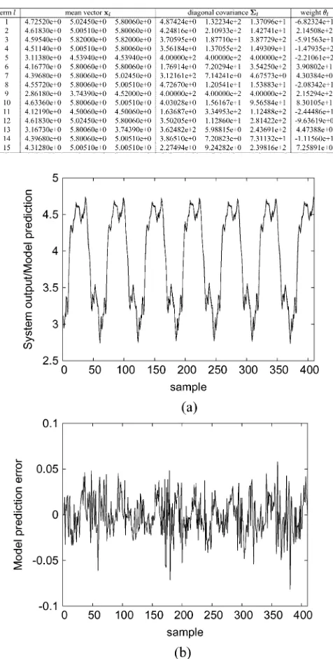
Fig. 2. Performance of the 15-term generalized Gaussian kernel model for the engine data set. (a) Model prediction^y (dashed) superimposed on the system outputy (solid). (b) Model prediction error = y 0 ^y .
Step 2) Update using (25) and (26) with . If remains sufficiently unchanged in two successive it-erations or a preset maximum iteration number (e.g., 10) is reached, stop; otherwise set and go to Step 1).
Fig. 3. Performance of the 15-term generalized Gaussian kernel model for the engine data set. (a) Iterative model output^y (dashed) superimposed on the system outputy (solid). (b) Iterative model error = y 0 ^y .
not the usual training MSE. Thus, the subset model selection is directly based on the model generalization capability using a single training set, with the LR further enforcing sparsity. Moreover, the subset model selection is fully automatic, and the user does not require to specify a termination criterion.
IV. MODELINGEXAMPLES
Two real-data sets were used to demonstrate the effective-ness of the proposed approach for constructing sparse gener-alized kernel models. The population size and the maximum repeating times for fitting kernel covariance matrices were chosen empirically to ensure that the subset selection procedure could produce consistent final models with the same levels of modeling accuracy and model sparsity for repeating runs. Em-pirically, it was found that the values of and did not criti-cally influence the modeling result.
Example 1: This example constructed a model representing the relationship between the fuel rack position (input ) and the engine speed (output ) for a Leyland TL11 turbocharged, di-rect injection diesel engine operated at a low engine speed. De-tailed system description and experimental setup can be found in [34]. The data set, depicted in Fig. 1, contained 410 sam-ples. The first 210 data points were used in training and the last 200 points in model validation. The previous study [34] has
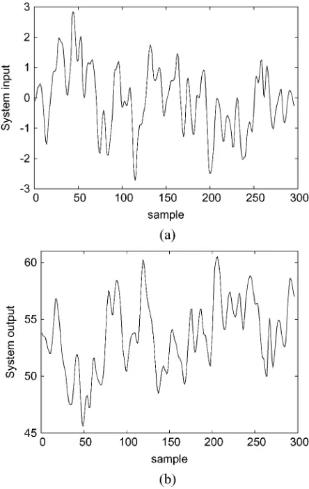
Fig. 4. Gas furnace data set. (a) System inputu . (b) System outputy .
shown that this data set can be modeled adequately by a non-linear model of the form
(33)
with describing the unknown underlying system and the system input vector defining by
(34)
Since every training input data points were considered as a can-didate regressor’s center, there were 210 regressors for the full regression model. The previous results [9], [10] had shown that when fitting a Gaussian kernel model with a single common variance, 1.69 was the optimal value for this kernel variance. Various kernel modeling techniques were em-ployed in [10] to fit this data set, and the best Gaussian kernel model was provided by the LROLS with the LOO test score, which consisted of 22 terms. The MSE values of this model over the training and validation sets were 0.000453 and 0.000490, respectively.
[image:6.594.317.539.64.415.2]TABLE II
SUBSETGENERALIZEDGAUSSIANKERNELMODELGENERATED FOR THEGASFURNACEDATASET BY THELROLS ALGORITHMWITH THELOO TESTSCORE. THE
KERNELCOVARIANCEMATRICESAREDETERMINED BYMAXIMIZING THECORRELATIONCRITERIONUSING THEREPEATEDWEIGHTEDOPTIMIZATIONALGORITHM
15-term subset generalized Gaussian kernel model from the re-sulting full regression matrix, and the constructed model is given in Table I. The MSE values of this model were 0.000482 over the training set and 0.000496 over the validation set, respectively. The model prediction and prediction error
generated by this model are illustrated in Fig. 2. The obtained 15-term generalized Gaussian kernel model was used to itera-tively generate the model output according to
(35)
with
(36)
where denotes the model mapping. The iterative model output and the iterative model error , are depicted in Fig. 3. Compared with the standard kernel method,
the proposed generalized kernel modeling approach is able to produce more parsimonious model with a similar modeling accuracy.
Example 2: This example constructed a model for the gas furnace data set [35, Series J]. The data set, illustrated in Fig. 4, contained 296 pairs of input–output points, where the input was the coded input gas feed rate and the output represented CO concentration from the gas furnace. All the 296 data points were used in training, with the model input vector defined by
(37)
Fig. 5. Performance of the 21-term generalized Gaussian kernel model for the gas furnace data set. (a) Model prediction ^y (dashed) superimposed on the system outputy (solid). (b) Model prediction error = y 0 ^y.
then used in [10] to fit a thin-plate-spline regression model for this data set, where the regressors were given by
(38)
and the best result obtained was again given by the LROLS with the LOO test score, which yielded a 28-term thin-plate-spline model with a training MSE of 0.053 306.
By adopting a generalized Gaussian kernel model structure, the LROLS with the LOO test score was able to identify a 21-term model, as listed in Table II, with a training MSE of 0.053 452. The candidate regressors’ kernel covariance ma-trices were fitted by optimizing the correlation criterion using the repeated weighted optimization with 21 and 10. The model prediction and prediction error generated by this 21-term generalized Gaussian kernel model are shown in Fig. 5. The obtained model was also used to iteratively produce the
model output given the input
(39)
The iterative model output and the associated modeling error are illustrated in Fig. 6.
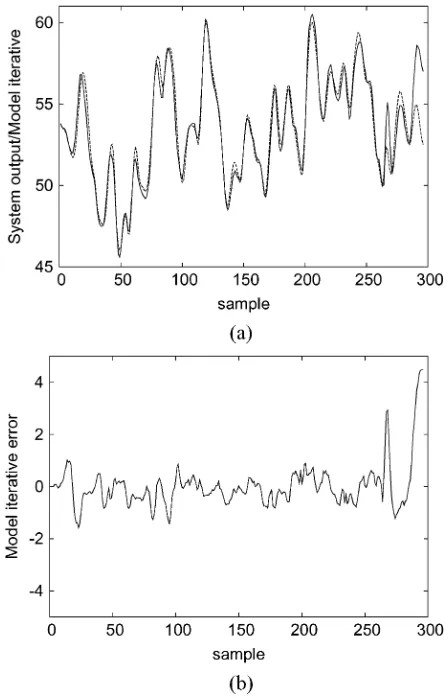
Fig. 6. Performance of the 21-term generalized Gaussian kernel model for the gas furnace data set. (a) Iterative model output^y (dashed) superimposed on the system outputy (solid). (b) Iterative model error = y 0 ^y .
V. CONCLUSION
Identification of discrete-time nonlinear systems has been considered using a generalized kernel regression model struc-ture. As with the standard kernel model, the kernel mean vectors are directly placed on the training input points. However, each regressor in the generalized kernel model has an individually fitted diagonal covariance matrix. This generalized kernel model structure, thus, has an enhanced modeling capability and is capable of producing more parsimonious models for nonlinear systems, compared with the standard kernel model structure. The design of the pool of regressors or the determi-nation of the candidate kernel covariance matrices is performed by maximizing a correlation criterion using a repeated guided random search based on boosting optimization. The efficient OLS algorithm based on the leave-one-out (LOO) test statistic and LR can then automatically select a sparse model from the resulting pool of candidate regressors. The effectiveness of the proposed nonlinear system identification approach has been demonstrated by the experimental results involving two real data sets.
APPENDIX
[image:8.594.316.540.63.412.2]Denote these models, identified using all the data points of , as and the corresponding modeling errors as
(40)
with index . A commonly used cross validation for model selection is the delete-one cross validation. The idea is as follows. For every model, each data point in the training set is sequentially set aside in turn, a model is estimated using the remaining data points, and the prediction error is de-rived using only the data point that was removed from training. Specifically, let be the resulting data set by removing the th data point from , and denote the th model estimated using as and the related predicted model residual at as
(41)
The mean square LOO test error [24], [27] for the th model is obtained by averaging all these prediction errors
(42)
The mean square LOO test error is a measure of the model gen-eralization capability. To select the best model from the can-didate models , the same modeling procedure is applied to each of the predictors, and the model with the minimum LOO test error is selected.
For linear-in-the-weights models, the LOO test errors can be generated, without actually sequentially splitting the training data set and repeatedly estimating the associated models, by using the Sherman–Morrison–Woodbury theorem [24]. More-over within the forward model selection procedure using the OLS algorithm, the LOO test errors for the -term model can be computed very efficiently. It can readily be shown [8], [10] that the computation of the LOO error for the -term model is based on the previously selected -term model and the currently selected th model term via the efficient re-cursion formulas (30) and (31).
The modified Gram–Schmidt orthogonalization procedure [2] calculates the matrix row by row and orthogonalizes as follows: at the th stage make the columns , orthogonal to the th column and repeat the operation for
. Specifically, denoting , ,
then for
(43)
The last stage of the procedure is simply . The elements of are computed by transforming in a similar way
(44)
This orthogonalization scheme can be used to derive a simple and efficient algorithm for selecting subset models in a forward-regression manner [2]. First define
(45)
If some of the columns in have been
interchanged, this will still be referred to as for no-tational convenience. Let a very small positive number be given, which specifies the zero threshold and is used to automat-ically avoiding any ill-conditioning or singular problem. With the initial conditions as specified in (32), the th stage of the se-lection procedure is given as follows.
Step 1) For :
Test—Conditioning number check. If , the th candidate is not considered.
Compute
and calculate, for ,
where and are the th elements of and , respectively. Let the index set be
Step 2) Find
Then the th column of is interchanged with the th column of , the th column of is interchanged with the th column of up to the
th row, and the th element of is interchanged with the th element of . This effectively selects the th candidate as the th regressor in the subset model.
Step 3) The selection procedure is terminated with a -term model, if . Otherwise, perform the orthogonalization as indicated in (43) to derive the th row of and to transform into ; calculate and update into in the way shown in (44); update the LOO error weightings
REFERENCES
[1] S. A. Billings and S. Chen, “The determination of multivariable non-linear models for dynamic systems,” inControl and Dynamic Systems, Neural Network Systems Techniques and Applications, C. T. Leondes, Ed. San Diego, CA: Academic, 1998, vol. 7, pp. 231–278.
[2] S. Chen, S. A. Billings, and W. Luo, “Orthogonal least squares methods and their application to nonlinear system identification,”Int. J. Control, vol. 50, no. 5, pp. 1873–1896, 1989.
[3] S. Chen, C. F. N. Cowan, and P. M. Grant, “Orthogonal least squares learning algorithm for radial basis function networks,” IEEE Trans. Neural Netw., vol. 2, no. 2, pp. 302–309, Mar. 1991.
[4] S. Chen, E. S. Chng, and K. Alkadhimi, “Regularised orthogonal least squares algorithm for constructing radial basis function networks,”Int. J. Control, vol. 64, no. 5, pp. 829–837, 1996.
[5] S. Chen, Y. Wu, and B. L. Luk, “Combined genetic algorithm opti-mization and regularised orthogonal least squares learning for radial basis function networks,”IEEE Trans. Neural Netw., vol. 10, no. 5, pp. 1239–1243, Sep. 1999.
[6] S. Chen, “Locally regularised orthogonal least squares algorithm for the construction of sparse kernel regression models,” inProc. 6th Int. Conf. Signal Processing, vol. 2, Beijing, China, Aug. 26–30, 2002, pp. 1229–1232.
[7] X. Hong and C. J. Harris, “Nonlinear model structure design and con-struction using orthogonal least squares and D-optimality design,”IEEE Trans. Neural Netw., vol. 13, no. 5, pp. 1245–1250, Sep. 2002. [8] X. Hong, P. M. Sharkey, and K. Warwick, “Automatic nonlinear
pre-dictive model construction algorithm using forward regression and the PRESS statistic,”Inst. Elect. Eng. Proc. Control Theory and Applica-tions, vol. 150, no. 3, pp. 245–254, 2003.
[9] S. Chen, X. Hong, and C. J. Harris, “Sparse kernel regression modeling using combined locally regularized orthogonal least squares and D-op-timality experimental design,”IEEE Trans. Autom. Control, vol. 48, no. 6, pp. 1029–1036, Jun. 2003.
[10] S. Chen, X. Hong, C. J. Harris, and P. M. Sharkey, “Sparse modeling using orthogonal forward regression with PRESS statistic and regular-ization,”IEEE Trans. Syst., Man, Cybern. B, Cybern., vol. 34, no. 2, pp. 898–911, Apr. 2004.
[11] V. Vapnik,The Nature of Statistical Learning Theory. New York: Springer-Verlag, 1995.
[12] V. Vapnik, S. Golowich, and A. Smola, “Support vector method for func-tion approximafunc-tion, regression estimafunc-tion, and signal processing,” in Ad-vances in Neural Information Processing Systems 9, M. C. Mozer, M. I. Jordan, and T. Petsche, Eds. Cambridge, MA: MIT Press, 1997, pp. 281–287.
[13] P. M. L. Drezet and R. F. Harrison, “Support vector machines for system identification,” inProc. UKACC Int. Conf. Control, Swansea, MA, U.K., Sep. 1–4, 1998, pp. 688–692.
[14] N. Cristianini and J. Shawe-Taylor,An Introduction to Support Vector Machines. Cambridge, U.K.: Cambridge Univ. Press, 2000. [15] M. E. Tipping, “Sparse Bayesian learning and the relevance vector
ma-chine,”J. Mach. Learn. Res., vol. 1, pp. 211–244, 2001.
[16] B. Schölkopf and A. J. Smola,Learning with Kernels: Support Vector Machines, Regularization, Optimization, and Beyond. Cambridge, MA: MIT Press, 2002.
[17] K. L. Lee and S. A. Billings, “Time series prediction using support vector machines, the orthogonal and the regularized orthogonal least-squares algorithms,”Int. J. Syst. Sci., vol. 33, no. 10, pp. 811–821, 2002. [18] L. Zhang, W. Zhou, and L. Jiao, “Wavelet support vector machine,”IEEE
Trans. Syst., Man, Cybern. B, Cybern., vol. 34, no. 1, pp. 34–39, Feb. 2004.
[19] W. Chu, S. S. Keerthi, and C. J. Ong, “Bayesian support vector regres-sion using a unified loss function,”IEEE Trans. Neural Netw., vol. 15, no. 1, pp. 29–44, Jan. 2004.
[20] R. E. Schapire, “The strength of weak learnability,”Mach. Learn., vol. 5, no. 2, pp. 197–227, 1990.
[21] Y. Freund and R. E. Schapire, “A decision-theoretic generalization of on-line learning and an application to boosting,”J. Comput. Syst. Sci., vol. 55, no. 1, pp. 119–139, 1997.
[22] G. Ridgeway, D. Madigan, and T. Richardson, “Boosting methodology for regression problems,” inProc. Artificial Intelligence and Statistics Conf., D. Heckerman and J. Whittaker, Eds., 1999, pp. 152–161. [23] R. Meir and G. Rätsch, “An introduction to boosting and leveraging,” in
Advanced Lectures in Machine Learning, S. Mendelson and A. Smola, Eds. Berlin, Germany: Springer-Verlag, 2003, pp. 119–184.
[24] R. H. Myers,Classical and Modern Regression with Applications, 2nd ed. Boston, MA: PWS-Kent, 1990.
[25] D. H. Wolpert, “Stacked generalization,”Neural Netw., vol. 5, no. 2, pp. 241–259, 1992.
[26] L. Breiman, “Stacked regressions,”Mach. Learn., vol. 24, pp. 49–64, 1996.
[27] L. K. Hansen and J. Larsen, “Linear unlearning for cross-validation,”
Adv. Computat. Math., vol. 5, pp. 269–280, 1996.
[28] G. Monari and G. Dreyfus, “Withdrawing an example from the training set: An analytic estimation of its effect on a nonlinear parameterised model,”Neurocomput., vol. 35, pp. 195–201, 2000.
[29] , “Local overfitting control via leverages,”Neural Computat., vol. 14, pp. 1481–1506, 2002.
[30] S. Chen and S. A. Billings, “Representation of nonlinear systems: The NARMAX model,”Int. J. Control, vol. 49, no. 3, pp. 1013–1032, 1989. [31] S. A. Billings and S. Chen, “Extended model set, global data and threshold model identification of severely nonlinear systems,”Int. J. Control, vol. 50, no. 5, pp. 1897–1923, 1989.
[32] S. Chen, X. X. Wang, and C. J. Harris, “Experiments with repeating weighted boosting search for optimization in signal processing applica-tions,” IEEE Trans. Syst., Man, Cybern. B, Cybern., Jun. 2005, to be published.
[33] D. J. C. MacKay, “Bayesian interpolation,”Neural Computat., vol. 4, no. 3, pp. 415–447, 1992.
[34] S. A. Billings, S. Chen, and R. J. Backhouse, “The identification of linear and nonlinear models of a turbocharged automotive diesel en-gine,”Mech. Syst. Signal Process., vol. 3, no. 2, pp. 123–142, 1989. [35] G. E. P. Box and G. M. Jenkins,Time Series Analysis, Forecasting and
Control. San Francisco, CA: Holden Day, 1976.
Sheng Chen(SM’97) received the B.Eng. degree in control engineering from the East China Petroleum Institute, Dongying, China, in 1982 and the Ph.D. de-gree in control engineering from the City University, London, U.K., in 1986.
He joined the School of Electronics and Computer Science, University of Southampton, Southampton, U.K., in 1999. He previously held research and aca-demic appointments at the University of Sheffield, Sheffield, U.K., the University of Edinburgh, Edinburgh, U.K., and University of Portsmouth, Portsmouth, U.K. His recent research works include adaptive nonlinear signal processing, modeling and identification of nonlinear systems, machine learning and neural networks, finite-precision digital controller design, evolutionary computation methods, and optimization. He has published over 200 research papers.
Dr. Chen is on the list of the highly cited researchers in the category that covers all branches of engineering subjects. In the database of the world’s most highly cited researchers in various disciplines, compiled by Institute for Scien-tific Information (ISI) of the USA.
Xia Hong(SM’02) received the B.Sc. and M.Sc. degrees from National University of Defense Technology, Changsha, China, in 1984 and 1987, respectively, and the Ph.D. degree from the Uni-versity of Sheffield, Sheffield, U.K., in 1998, all in automatic control.
She worked as a Research Assistant at the Beijing Institute of Systems Engineering, Beijing, China, from 1987 to 1993. She worked as a Research Fellow in the Department of Electronics and Computer Sci-ence, University of Southampton, Southampton, U.K., from 1997 to 2001. She is currently a Lecturer in the Department of Cybernetics, University of Reading, Reading, U.K. She is actively engaged in research into neurofuzzy systems, data modeling, and learning theory and their applications. Her research interests include system identification, estimation, neural networks, intelligent data modeling, and control. She has published over 40 research papers, and coauthored a research book.
Chris J. Harrisreceiving the B.Sc. degree from the University of Leicester, Leicester, U.K., the M.A. degree from the University of Oxford, Oxford, U.K., and the Ph.D. degree from the University of Southampton, Southampton, U.K.
He previously held appointments at the University of Hull, Hull, U.K., the UMIST, Manchester, U.K., the University of Oxford, Oxford, U.K., and the Uni-versity of Cranfield, Cranfield, U.K., as well as being employed by the U.K. Ministry of Defense. He re-turned to the University of Southampton as the Lucas Professor of Aerospace Systems Engineering in 1987 to establish the Advanced Systems Research Group and, more recently, Image, Speech and Intelligent Sys-tems Group. His research interests lie in the general area of intelligent and adap-tive systems theory and its application to intelligent autonomous systems such as autonomous vehicles, management infrastructures such as command & con-trol, intelligent concon-trol, and estimation of dynamic processes, multisensor data fusion, and systems integration. He has authored and coauthored 12 research books and over 300 research papers, and he is the associate editor of numerous international journals.
Dr. Harris was elected to the Royal Academy of Engineering in 1996, was awarded the Institution of Electrical Engineers (IEE) Senior Achievement medal in 1998 for his work in autonomous systems, and the highest international award in IEE, the IEE Faraday medal, in 2001 for his work in intelligent control and neurofuzzy systems.
Xunxian Wangreceived the Ph.D. degree in the con-trol theory and application field from Tsinghua Uni-versity, Beijing, China, in 1999.