Effects of Rate Adaptation on the Throughput of Random Ad Hoc Networks
Xiang Liu and Lajos Hanzo
School of ECS, University of Southampton, SO17 1BJ, UK.
Tel: +44-23-8059-3125, Fax: +44-23-8059-4508
Email:[email protected]
,
http://www-mobile.ecs.soton.ac.uk
Abstract
The capacity of wireless ad hoc networks has been studied in an excellent treatise by Gupta and Ku-mar [1], assuming a fixed transmission rate. By con-trast, in this treatise we investigate the achievable throughput improvement ofrate adaptationin the con-text of randomad hocnetworks, which have been stud-ied in conjunction with afixed transmission ratein [1]. Our analysis shows thatrate adaptationhas the poten-tial of improving the achievable throughput compared
tofixed rate transmission, since rate adaptation
miti-gates the effects of link quality fluctuations. However, even perfect rate control fails to change the scaling law of the per-node throughput result given in [1], regard-less of the absence or presence of shadow fading. This result is confirmed in the context of specific adaptive modulation aided design examples.
1. INTRODUCTION
An ad hoc network consists of a number of mobile nodes, which may communicate directly with each other over wire-less links, but anad hoc network has no base station infras-tructure. One of the most important characteristics ofad hoc
networks is their achievable capacity [1]. More specifically, in their landmark paper [1] Gupta and Kumar studied the achievable capacity ofad hoc networks havingnnodes, each capable of transmitting atW bits per second. Two types of network models were considered in their work,arbitrary net-works, which consist of arbitrarily located nodes generating an arbitrary traffic pattern, andrandom networks, which consist of randomly located nodes generating a random traffic pat-tern. The results of [1] showed that the throughput achiev-able by each node was Θ(W/√n)1 forarbitrary networks and Θ(W/√nlogn) forrandom networks. Both of these formulae implied that the per-node throughput tended to zero, as the number of nodes tended to infinity.
Directional and other types of smart antennas have also been used for increasing the achievable capacity of wirelessad hocnetworks [2,3]. It was shown [2,3] that thescalability prob-lem2might be mitigated by increasing the number of antenna elements and the resultant antenna gain, which is a benefit of having a narrower beam-width. However, despite its consid-erable complexity, beamforming does not dramatically change
The financial support of the European Union under the auspices of the Phoenix and Newcom projects as well as of the EPSRC, UK is gratefully acknowledged.
1The function Θ(W/√n) returns a value, which is not much
worse, but also not much better thanW/√n.
2Scalability in ad hoc networks implies that whether the
net-work is capable of providing an acceptable level of service, when the number of nodes in the network tends to infinity [4].
the scaling law3 due to the limitations of realistic systems [3]. It was also shown [5] that terminal mobility was capable of increasing the per-node throughput to Θ(1) with the aid of a two-hop strategy, even when the number of communicating nodesnwas high, provided that the transmission delay was not taken into account, which is a somewhat irrealistic assumption. However, the expected delay per packet imposed by the above strategy might be Θ(logn) [6], which suggests that mobilead hoc networks constituted by many nodes may not be scalable in real-time applications.
The capacity of hybrid wireless networks, which consist ofad hoc nodes benefitting from infrastructure support, was studied in [7,8]. The results showed that the per-node through-put of ad hoc networks was improved by the infrastructure support provided by both regular base stations [7] and ran-dom distributed access points [8].
A mathematical framework was defined for studying the capacity of wirelessad hocnetworks in [9]. The results showed that multihop routing, spatial reuse4, successive interference cancellation (SIC) and variable-rate transmissions hold the promise of significantly improving the achievable capacity. Both terminal mobility and fading were also found to increase the achievable network capacity, provided that nodes were capa-ble of tolerating large delays, since the network was allowed to schedule its transmissions during favourable fading or mobility conditions.
In most of the above mentioned literature, afixed transmis-sion rateassociated with a time-invariant modulation scheme was assumed [1–3,5,7,8]. Toumpis and Goldsmith numerically characterized the effects ofrate adaptation with the aid of a rigorous mathematical framework [9], stating that the associ-ated computational complexity of scheduling would increase exponentially, as the number of nodes increased.
In this paper, the effect ofrate adaptation on the achiev-able per-node throughput ofad hocnetworks will be estimated. In Section 2, the system model of wirelessad hocnetworks is introduced. In Section 3, the achievable throughput improve-ments of perfect rate adaptation are estimated without tak-ing into account the effects of fadtak-ing. To expound further, in Section 4 the effect of perfectrate adaptation under shadow-ing is analyzed. Examples of Adaptive Quadrature Amplitude Modulation (AQAM) simulations are provided in Section 5. Finally, Section 6 provides our conclusions.
3The scaling law inad hocnetworks characterizes how the
net-work performance varies, as the number of nodes in the netnet-work tends to infinity. In this treatise the network performance is mea-sured by the achievable per-node throughput.
4Spatial reuse implies that more than one nodes are allowed to
attempt the simultaneous transmission of a given packet towards its destination.
Crown Copyright 2005
2. SYSTEM MODEL
Our model of thead hocnetwork considered is similar to that used in [1], apart from a few modifications, which include the employment of perfect rate adaptation and the effects of a fading channel.
Let us consider a random ad hoc network supporting n nodes uniformly and independently distributed in a unit area
S, which is a planar disk as in [1]. All nodes share the same bandwidth, which is given byW Hz. All packet-transmissions are slotted into perfectly synchronized time slots. No node is capable of simultaneously transmitting and receiving signals, or simultaneously transmitting/receiving signals to/from more than one node. The power of each transmitting node is fixed toPt Watts, i.e. no power control is used, which is typical in
cost-efficientad hoc networks.
LetNtbe the subset of nodes simultaneously transmitting at some time instant. If node i, i /∈ Nt is receiving signals
from nodej,j∈ Nt, then the Signal-to-Interference-plus-Noise
Ratio (SINR) experienced at nodeibecomes:
γji= PtGji
k∈Nt,k=jPtGki+ηi
, (1)
where γji is the SINR at node i experienced by the signal
arriving from node j, while Gki is the power gain between nodesk andi, while ηi is the background noise encountered at node i. The value of the power gainGji depends on the
propagation model, which will be discussed in Sections 3 and 4, taking into account the absence of fading or the presence of log-normal shadow fading, respectively. The minimum SINR required for successful reception isβ, as defined in [1].
Every transmitting node assumes perfect knowledge of its link quality and hence we are estimating the achievable through-put upper bound with the advent of perfect adaptive rate transmission, which is a prerequisite for approaching the Shan-non limit [10].
The common reliable transmission range r(n) of all nodes is chosen to guarantee the asymptotic connectivity of random networks as in [1]. The shorthand ofrn will be used forr(n) in the sequel. Initially the minimum distance between nodes is assumed to bermin, which satisfiesrmin< rn, although later
this assumption will be dropped, lettingrmin→0.
3. THE EFFECTS OF PATH LOSS
In the absence of fading, i.e. when the only propagation phe-nomenon considered is the path loss, the signal power is as-sumed to decay upon increasing the distance r according to r−α
, yielding:
G(r) =r−α, (2)
whererandG(r) are the distance and the power gain between two nodes, respectively, and αis the path loss exponent. In general we have 2≤α≤4 in a typical path loss model [11].
Let us assume that nodejis transmitting to nodei roam-ing at a distance less thanrn. Owing to the central limit
the-orem, the interference may be assumed to be approximately Gaussian. Thus only the fluctuation of the received signal power is considered.
In the model of [1], the guard zone5 is appropriately se-lected to guarantee that all nodes’ transmissions to other nodes roaming at a distance less than rn achieve the minimum
re-quired SINRβ, so that we haveγji=β
rn rji
α
.
5A guard zone is specified as a transmission exclusion zone
im-posed for the sake of preventing a neighbouring node from trans-mitting on a channel already activated within the zone at the same time.
In the model of [1], the transmission rate is fixed. Hence the throughputcg achievable without rate adaptation is also fixed and determined by the Shannon limit [10] at the mini-mum required SINRβ, yieldingcg=Wlog2(1 +β).
Since nodejis randomly and uniformly distributed inS, furthermore, given thatrji is less than the reliable range of
transmissionrn, the conditional Probability Density Function
(PDF) of the distancerjiand the conditional PDF of the SINR γjican be shown to be:
fr|r<rn(rji) = 2rji r2
n−r2min, r
min< rji< rn, (3)
fγ|r<rn(γji) = 2
γ
ji
β
−2 α−1
αβ
1−rmin
rn
2, β < γji. (4)
If perfectrate adaptationis available, the achievable aver-age throughputcacan be shown to be:
ca= 2W
(r2n−r2min) ln 2
rn
rminr jiln
1 +β
rn
rji
α
drji. (5)
Hence it is possible to estimate the achievable normalized per-node throughput improvement ofci=ca/cgattained with the advent of perfect rate adaptation by numerical integra-tion. Upon substituting the normalized minimum distance of u=rmin/rnbetweenad hoc nodes as well as the normalized distances=rji/rn into Equation 5, we arrive at the
follow-ing theorem quantifyfollow-ing the normalized per-node throughput improvement in the absence of fading.
Theorem 1
ci = ca cg =
2 u1sln(1 +βs−α)ds (1−u2) ln(1 +β) ≤
2 01sln(1 +βs−α)ds ln(1 +β)
= c0i <+∞, (6)
where the upper boundc0i is the maximum achievable
normal-ized throughput improvement ci attained with the advent of perfect rate adaptation, when we havermin= 0.
Note in Equation 6 that the upper boundc0i is a constant
that is independent ofn, and it is determined purely by the propagation parameters,αandβ. Therefore, it is concluded thatcahas the same order ascg, which is the achievable per-node throughput in the model of [1]. In other words, even perfectrate adaptation fails to change the scaling law of the achievable per-node throughput result of [1].
Figures 1 and 2 show that the achievable normalized per-node throughput improvement ci is a decreasing function of
the normalized minimum distance rmin/rn. In other words, as the minimum distance between nodes decreases, the achiev-able normalized per-node throughput improvement increases, because the link quality fluctuation becomes larger at a smaller normalized minimum distance between nodes, whilefixed rate transmissionfails to efficiently exploit the available capacity, when the link quality is improved.
4. THE EFFECTS OF SHADOW FADING
If the effects of shadowing are taken into account, the shadow-faded power gain is log-normally distributed with a mean given by Equation 2. Then the conditional PDF of the shadow-faded power gain at a certain distance is given by [11]:
fG|r(G) =√ 1
2πσGe
−(lnG+αlnr)2
2σ2 , (7)
0.0 0.1 0.2 0.3 0.4 0.5 0.6 0.7 0.8 0.9 1.0
Normalized minimum distance between nodes, rmin/rn 1.0
1.2 1.4 1.6 1.8 2.0 2.2 2.4
Normalized
throughput
improvement,
ci
[image:3.595.327.509.93.231.2]=10 dB =4 =3 =2
Figure 1: The normalized per-node throughput improvement ci versus the normalized minimum distance rmin/rn between nodes for different values of the path loss exponentαat a required SINR value ofβ= 10 dB in the absence of fading, which is computed from Equation 6.
0.0 0.1 0.2 0.3 0.4 0.5 0.6 0.7 0.8 0.9 1.0
Normalized minimum distance between nodes, rmin/rn 1.0
1.5 2.0 2.5 3.0 3.5 4.0
Normalized
throughput
improvement,
ci
=20 dB =10 dB =0 dB =3
Figure 2: The normalized per-node throughput improvement ci versus the normalized minimum distance rmin/rn between nodes for different values of the required SINRβat a path loss exponent of
α= 3 in the absence of fading, which is computed from Equation 6.
whereGandr are the power gain and the distance between two nodes, respectively andσis the standard deviation of the lognormal shadowing in natural units. In practice the range of σ is 5∼12 dB and its typical value is 8 dB [11], i.e. we have 1.15∼2.76 and 1.84 in terms of natural units.
Owing to the central limit theorem, the interference is ap-proximatively Gaussian distributed. Hence only the fluctua-tion of the shadow-faded received signal power is considered. The guard zone is appropriately selected to guarantee that all nodes’ transmissions to other nodes roaming at a distance less than rn achieve the minimum required SINR β on average, hence we have:
γji=βrnαGji, (8)
where the shadow-faded power gain Gji is log-normally dis-tributed with a mean ofr−jiα.
Substituting Equation 8 into Equation 7 and applying the probability transformation formula [12], we have the condi-tional PDF ofγjiat a given distancerji:
fγ|rji(γji) =√ 1 2πσγjie
−(lnγji+αlnrji2σ−2lnβ−αlnrn)2. (9)
Upon substituting Equation 3 into Equation 9 and apply-ing the theorem of total probability [12], we arrive at the PDF ofγjiconditioned onrji< rn:
fγ|rji<rn(γji) =
2 rrn
minrjie
−(lnγji+αlnrji2−lnβ−αlnrn)2 σ2 drji
√
2πσγji(r2n−r2min)
.
(10)
0.0 0.1 0.2 0.3 0.4 0.5 0.6 0.7 0.8 0.9 1.0
Normalized minimum distance between nodes, rmin/rn 1.0
1.2 1.4 1.6 1.8 2.0 2.2 2.4
Normalized
throughput
improvement,
ci
[image:3.595.68.252.280.420.2]=8 dB =10 dB =4 =3 =2
Figure 3: The normalized per-node throughput improvement ci versus the normalized minimum distance rmin/rn between nodes for different values of the path loss exponentαat a required SINR value ofβ= 10 dB and a lognormal shadowing standard deviation ofσ= 8 dB in the presence of shadow fading, which is computed from Equation 12.
Therefore the normalized per-node throughput improve-mentci achieved with the aid of perfectrate adaptationmay be expressed as follows:
ci=ca cg =
∞
β fγ|r<rn(γji) ln(1 +γji)dγji
ln(1 +β) β∞fγ|r<rn(γji)dγji . (11)
Upon substituting the logarithmic normalized minimum distance ofu= lnrmin−lnrn betweenad hocnodes as well as the logarithmic normalized distance of s = lnrji−lnrn
and the logarithmic normalized SINR oft= lnγji−lnβinto Equation 11, we arrive at the following theorem in the presence of shadow fading.
Theorem 2
ci =
+∞
0 ln(1 +βet)dt 0
ue2se−
(t+αs)2 2σ2 ds
ln(1 +β) 0+∞dt u0e2se−(t+αs)22σ2 ds
≤
+∞
0 ln(1 +βe
t
)dt −∞0 e2se−(t+αs)22σ2 ds
ln(1 +β) 0+∞dt −∞0 e2se−(t+αs)22σ2 ds
= c0i <+∞, (12)
where the upper boundc0i experienced in the presence of shadow
fading is the maximum achievable normalized throughput im-provementci attained with the advent of perfect rate
adapta-tion, when we havermin= 0.
Observe in Equation 12 that the upper boundc0i is still a
constant, regardless of the specific value ofn, and it is purely determined by the propagation parametersα,βandσ. There-fore, it is concluded thatca has the same order ascg, which
is the achievable throughput in the model of [1]. In other words, perfectrate adaptation fails to change the scaling law of the per-node throughput result of [1], even in the presence of shadow fading.
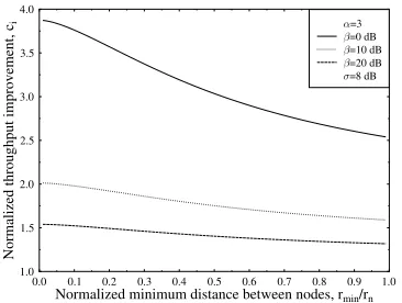
Figures 3 - 5 show that the achievable normalized per-node throughput improvementciexperienced in the presence
of shadow fading is also a decreasing function of the normalized minimum distancermin/rn, and this trend is similar to that in the absence of shadowing, as it was evidenced by Figures 1 and 2. However, the achievable normalized per-node throughput improvement ci is higher than unity even at rmin/rn = 1, which is different from that in the absence of shadowing. This
[image:3.595.322.546.434.534.2]0.0 0.1 0.2 0.3 0.4 0.5 0.6 0.7 0.8 0.9 1.0
Normalized minimum distance between nodes, rmin/rn 1.0
1.5 2.0 2.5 3.0 3.5 4.0
Normalized
throughput
improvement,
ci
[image:4.595.70.253.93.231.2]=8 dB =20 dB =10 dB =0 dB =3
Figure 4: The normalized per-node throughput improvement ci versus the normalized minimum distance rmin/rn between nodes for different values of the required SINRβat a path loss exponent value of α= 3 and a lognormal shadowing standard deviation of
σ= 8 dB in the presence of shadow fading, which is computed from Equation 12.
0.0 0.1 0.2 0.3 0.4 0.5 0.6 0.7 0.8 0.9 1.0
Normalized minimum distance between nodes, rmin/rn 1.0
1.2 1.4 1.6 1.8 2.0 2.2 2.4
Normalized
throughput
improvement,
ci
[image:4.595.69.251.292.427.2]=12 dB =8 dB =5 dB =10 dB =3
Figure 5: The normalized per-node throughput improvement ci versus the normalized minimum distance rmin/rn between nodes for different values of the lognormal shadowing standard deviation
σ at a path loss exponent value ofα= 3 and a required SINR of
β = 10 dB in the presence of shadow fading, which is computed from Equation 12.
gain was achieved by counteracting the link quality variation imposed by shadow fading, regardless of the normalized node separation. Observe in Equation 12 that at rmin/rn = 1 we
have:
ci|rmin rn =1=
+∞
0 ln(1 +βet)e−
t2 2σ2dt
ln(1 +β) 0+∞e− t
2 2σ2dt
>1. (13)
We observe from Equation 13 that the normalized per-node throughput improvementci achieved atrmin/rn= 1 is
inde-pendent of the path loss exponent α, and it is purely deter-mined by the required minimum SINR β as well as the log-normal shadowing standard deviationσ. This is because the conditional PDF of γji at a given distance rji does not
de-pend onαatrmin=rn, as observed in Equation 9. Hence the curves associated with different values of αin Figure 3 con-verge, when we have rmin →rn, but this is not the case for
different values ofβ, as seen in Figure 4 or for different values ofσ, as portrayed in Figure 5.
5. EXAMPLE: AQAM
The family of AQAM schemes constitutes an efficient rate
adaptationtechnique designed with low complexity in mind for the sake of increasing the achievable throughput [13]. There are several criteria that may be invoked for choosing the switch-ing levels between the adjacent AQAM modes [13, 14]. In the
previous sections we used the idealized concept of instanta-neous SINR channel quality knowledge for evaluating the ben-eficial effects of perfectrate adaptation on the achievable ef-fective throughput upper bound.
In this section a K-mode adaptive square QAM scheme using Gray coding is investigated. The mode selection rule is formulated as follows [14]:
Choose modek, when we havesk≤γs< sk+1, k∈ {0, ..., K}, whereγs is the instantaneous SNR per symbol,skis thekth
switching level ands0= 0,sK+1=∞. The AQAM constella-tion size is given byMkphasors in modekas follows:
M0= 0, M1= 2, Mk= 22(k−1), k= 2, ..., K. The number of bits per symbol (BPS)bktransmitted in mode
kis given by:
b0= 0, bk= log2Mk, k= 1, ..., K.
The general BER expression ofM-ary square QAM using Gray coding is given by Equation 14 and 16 in [15], where γ= γs
log2M is the SNR per bit. Hence we arrive at the AQAM
parameters listed in Table 1, which are independent of the associated SNR distribution. For example, if a 5-mode square AQAM scheme is adopted, the maximum constellation size will beM5= 256 and the highest switching level becomess6=∞,
regardless of the target BER.
The average number of bits per symbol normalized to that of the fixed rate BPSK scheme is [14]:
Bi= K
k=1bk ssk+1
k fγs(γs)dγs
BBPSK , (14)
wherefγs(γs) is the PDF of the SNR per symbol andBBPSK
is the BPS throughput of the fixed rate BPSK scheme. In general a constant symbol rate is used in AQAM, regardless of the modulation mode selected, hence a constant bandwidth is required. Again, if we treat the co-channel interference as noise, which is justified by the central limit theorem,fγs(γs) is
given by Equations 4 and 10 in the absence and in the presence of shadowing, respectively. The PDFs of their normalized val-ues associated withrmin = 0 are depicted in Figure 6. Since
the SINR achieved at the fringes of the transmission rangern
exactly satisfies the minimum SINR requirementβ, provided that only the effect of path loss is considered, the SINR nor-malized to β is always higher than or equal to 0 dB in the absence of fading, as suggested by Figure 6. The peak value of the SINR PDF is reached at a normalized SINR value of less than 0 dB in the presence of shadowing, because the abscissa value of the peak r−αe−σ2 of the lognormal distribution in Equation 7 is less than the SINR’s mean value ofr−αe−σ2/2. The achievable normalized average BPS throughputBiversus
the number of modesK of K-mode square AQAM systems
associated withrmin = 0 andβ=s1 is characterized in
Fig-ure 7, which was recorded both in the absence of fading and in the presence of shadowing.
Figure 7 shows that AQAM is capable of substantially im-proving the average BPS throughput both in the absence of fading and in the presence of shadowing compared to the fixed rate BPSK scheme. However, the additional throughput im-provement achieved by a high-complexity scheme using more than four AQAM modes is marginal, because the probability of activating the high-BPS modes drops exponentially, when the SINR normalized toβincreases, as suggested by the PDF seen in Figure 6. This result is in line with Theorem 1 and The-orem 2, suggesting that even perfect rate adaptation is inca-pable of improving the scaling law of the per-node throughput
k 0 1 2 3 4 5 6
Mk 0 2 4 16 64 256 1024
bk 0 1 2 4 6 8 10
sk(dB) BER = 10−3 −∞ 6.7895 9.7998 16.5430 22.5490 28.4147 34.2607
[image:5.595.107.489.74.133.2]sk(dB) BER = 10−5 −∞ 9.5879 12.5982 19.4551 25.5684 31.5341 37.4728 mode No Tx BPSK QPSK 16-QAM 64-QAM 256-QAM 1024-QAM
Table 1: The parameters ofK-mode square AQAM systems using Gray coding and designed for maintaining BER = 10−3 and 10−5, respectively. The switching thresholds were evaluated from Equations 14, 16 in [15] andγ=γs/log2M.
-40 -30 -20 -10 0 10 20
Normalized SINR, s/ (dB) 0.0
0.1 0.2 0.3 0.4 0.5 0.6 0.7
Probabilty
[image:5.595.71.252.170.304.2]SINR’s PDF in the presence of shadowing SINR’s PDF in the absence of fading
Figure 6: The PDFs of the SINRs normalized to the minimum SINR requirementβboth in the absence of fading and in the pres-ence of log-normal shadowing having α= 3 and σ= 8 dB, which were computed from Equations 4 and 10 forrmin= 0, respectively.
1 2 3 4 5 6
Number of AQAM modes, K
0.0 0.5 1.0 1.5 2.0 2.5 3.0 3.5 4.0
Normalized
BPS
throughput,
Bi
K-mode AQAM, BER=10-5, in the presence of shadowing K-mode AQAM, BER=10-3, in the presence of shadowing K-mode AQAM, BER=10-5, in the absence of fading K-mode AQAM, BER=10-3, in the absence of fading
Figure 7: The achievable normalized per-node average BPS throughputBi versus the number of modesK in K-mode square AQAM systems using Gray coding for a path loss exponent value of
α= 3, a lognormal shadowing standard deviation ofσ= 8 dB and a target BER of 10−3 and 10−5, respectively, recorded both in the absence of fading and in the presence of shadow fading in a random
ad hoc network. The PDFfγs(γs) of the SNR per symbol is given by Equation 10 and Equation 10, respectively.
attained either in the absence of fading or in the presence of shadowing. The achievable normalized average BPS through-put recorded in the case of a higher threshold set designed for maintaining BER ≥10−5 is only marginally lower than that in the case of a lower threshold set designed for maintaining BER≥10−3, since the distributions of the normalized SINR of the BER = 10−5 and 10−3 scenarios are identical, as seen in Figure 6. This implies that a lower BPS throughput im-provement may be achieved in case of requiring a lower BER of 10−5, which conforms to the trends observed in Figure 2. However, it does not imply that the AQAM scheme achieves a lower BPS throughput in the case of aiming for a lower instan-taneous BER, since we normalize the BPS throughput to that of the fixed rate BPSK scheme, which is different for the sce-narios of BER = 10−3and BER = 10−5owing to the different values ofrn.
6. CONCLUSION
In this paper we have focused our attention on the effects of
rate adaptation on the achievable throughput of random ad hocnetworks, which was discussed in the context of both path loss and shadow fading. In conclusion, perfectrate adapta-tion has the potential of considerably improving the achiev-able throughput of the randomad hoc network compared to
fixed rate transmissions, since rate adaptation is capable of mitigating the effects of link quality fluctuations, as shown in Figures 1 - 5. However, Theorem 1 and 2 revealed that even perfect rate control fails to change the scaling law of the per-node throughput result given by Θ
1
√
nlogn
in [1], regardless of the absence or presence of shadow fading. This conclu-sion was further confirmed by Figure 7 in the context of our AQAM examples. The maximum normalized throughput im-provementc0i achieved with the aid of perfectrate adaptation
is determined purely by the path loss exponentα, the required
minimum SINRβand the lognormal shadowing standard
de-viationσ. We observed in Figures 1, 3 and 5 that the achiev-able normalized throughputc0i increases, asαorσincreases,
because it is capable of efficiently mitigating the link quality variations. More explicitly, this was demonstrated in Figure 1 in the absence of fading, while in Figures 3 and 5 in the pres-ence of shadowing, respectively. By contrast,c0i decreases as
βdecreases, as a consequence of the reduced marginal channel throughput, as shown in Figure 2 in the absence of fading and in Figure 4 in the presence of shadowing, respectively.
7. REFERENCES
[1] P. Gupta and P. Kumar, “The capacity of wireless networks,”IEEE Transactions on Information Theory, vol. 46, pp. 388–404, March 2000.
[2] A. Spyropoulos and C. Raghavendra, “Capacity bounds for ad-hoc networks using directional antennas,” inIEEE International Conference on Communications, vol. 1, (Anchorage, Alaska, USA), pp. 348–352, 11-15 May 2003.
[3] A. Spyropoulos and C. Raghavendra, “Asympotic capacity bounds for ad-hoc networks revisited: the directional and smart antenna cases,” inIEEE Global Telecommunications Conference, vol. 3, (San Francisco, California, USA), pp. 1216–1220, 1-5 December 2003.
[4] R. Ramanathan and J. Redi, “A brief overview of ad hoc networks: challenges and directions,”IEEE Communications Magazine, vol. 40, pp. 20–22, May 2002. [5] M. Grossglauser and D. Tse, “Mobility increases the capacity of ad hoc wireless
networks,”IEEE/ACM Transactions on Networking, vol. 10, pp. 477–486, August 2002.
[6] D. S. Heberto del Rio, “Logarithmic expected packet delivery delay in mobile ad hoc wireless networks,”Wiley Journal on Wireless Communications and Mobile Computing, vol. 4, pp. 281–287, May 2004.
[7] B. Liu, Z. Liu, and D. Towsley, “On the capacity of hybrid wireless networks,” inIEEE INFOCOM, vol. 2, (San Francisco, Carlifornia, USA), pp. 1543 –1552, 30 March-3 April 2003.
[8] U. C. Kozat and L. Tassiulas, “Throughput capacity of random ad hoc net-works with infrastructure support,” inInternational Conference on Mobile Comput-ing and NetworkComput-ing, (San Diego, Carlifornia, USA), pp. 55–65, 14-19 September 2003.
[9] S. Toumpis and A. J. Goldsmith, “Capacity regions for wireless ad hoc net-works,”IEEE Transactions on Wireless Communications, vol. 2, pp. 736–748, July 2003.
[10] T. M. Cover and J. A. Thomas,Elements of information theory. John Wiley, 1991. [11] J. G. Proakis,Digital Communications. McGraw-Hill Companies, Inc., 4th ed.,
2001.
[12] E. Lloyd,Probability, vol. II ofHandbook of Applicable Mathematics. John Wiley & Sons Ltd., 1980.
[13] L. Hanzo, S. X. Ng, T. Keller, and W. Webb,Quadrature Amplitude Modulation: From Basics to Adaptive Trellis-Coded, Turbo-Equalised and Space-Time Coded OFDM, CDMA and MC-CDMA Systemss. John Wiley & Sons Ltd., 2 ed., November 2004. [14] B. Choi and L. Hanzo, “Optimum mode-switching-assisted constant-power single- and multicarrier adaptive modulation,”IEEE Transactions on Vehicular Technology, vol. 52, pp. 536–560, May 2003.
[15] K. Cho and D. Yoon, “On the general BER expression of one- and two-dimension amplitude modulations,”IEEE Transactions on Communications, vol. 50, pp. 1074–1080, July 2002.
[image:5.595.67.249.348.483.2]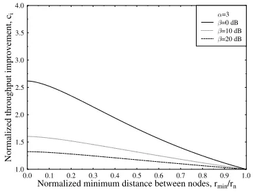
![Table 1: The parameters ofrespectively. The switching thresholds were evaluated from Equations 14, 16 in [15] and K-mode square AQAM systems using Gray coding and designed for maintaining BER = 10−3 and 10−5, γ = γs/ log2 M.](https://thumb-us.123doks.com/thumbv2/123dok_us/8511585.350261/5.595.71.252.170.304/parameters-ofrespectively-switching-thresholds-evaluated-equations-designed-maintaining.webp)
