Fast Norm-Optimal Iterative Learning Control for Industrial
Applications
James Ratcliffe, Lize van Duinkerken, Paul Lewin, Eric Rogers,
Jari Hätönen, Thomas Harte and David Owens
Abstract— Norm-Optimal Iterative Learning Control has potential to significantly increase the accuracy of many tra-jectory tracking tasks which can be found in industry. The algorithm can achieve very low levels of tracking error and the number of iterations required to reach minimal error is small compared to many other Iterative Learning Control Algorithms. However, in the current format, the algorithm is not attractive to industry because it requires a large number of calculations to be performed at each sample instant. This implies that control hardware must be very fast which is expensive, or that the sample frequency must be reduced which can result in reduced performance. To remedy these problems, a revised version, Fast Norm-Optimal Iterative Learning Control is proposed which is significantly simpler and faster to implement. The new version is tested both in simulation and in practice on a three axis industrial gantry robot.
I. INTRODUCTION
Iterative Learning Control (ILC) is a technique which is designed to improve the performance of tracking control systems which have a repeated reference trajectory. Such systems include food processing plants, assembly lines, chemical batch reactors and robotic arm manipulators. Each time the trajectory is implemented (known as a trial or iteration), ILC uses data from past iterations to modify the control signal in an attempt to reduce the tracking error obtained during the next iteration. Between each iteration there is an undefined stoppage time, during which the plant is reset to known initial states. ILC is theoretically capable of reducing the tracking error to zero as the number of iterations increases towards infinity [1]. This is a significant advantage over conventional algorithms where the same level of tracking error can be expected at each trial [2].
It is generally recognised that ILC was formally defined by Arimoto, Kawamura and Miyazaki in 1984 [3]. The first algorithm to be developed was very simple and consisted of a tracking error term and a previous iteration input term [4]. However, over the past 20 years there has been significant
This work was supported by the EPSRC contract no. GR/R74239/01 J. Ratcliffe, P. Lewin and E. Rogers are with the School of Electronics and Computer Science, University of Southampton, Uni-versity Road, Southampton, SO17 1BJ, United Kingdom, e-mail: [email protected](J. Ratcliffe)
L. van Duinkerken is with the Department of Applied Mathematics, Delft University of Technology, Mekelweg 4, 2628 CD, Delft, Netherlands J. Hätönen, T. Harte and D. Owens are with the Department of Auto-matic Control and Systems Engineering, University of Sheffield, Mappin Street, Sheffield, S1 3JD, United Kingdom
J. Hätönen is also with the Systems Engineering Laboratory, The University of Oulu, P.O. BOX 4300, FIN-90014 University of Oulu, Finland
development of ILC algorithms which now include prin-ciples and theory from a wide range of automatic control disciplines. Notably, there have been significant contribu-tions from Robust, Adaptive and Optimal control (see [5]– [7] for examples). Many of these ILC variations are highly advanced model-based systems which aim to maximise the tracking error reduction while still maintaining stability in the presence of unmodelled dynamics and non-repeating disturbances.
In the vast majority of cases, these advanced algorithms are evaluated with simulation experiments, which invariably conclude that the increased complexity of the algorithm is extremely well justified by the significant improvements in tracking error reduction and convergence rate, when compared to simpler algorithms which require no form of plant model. However there is rarely any consideration of the effect which the increased complexity of the algorithm will have on practical implementation of the algorithm on a real system. Modern control systems are almost exclu-sively implemented in sampled format on some form of digital electronic device, examples of which include single-chip micro-controllers, programmable-logic controllers and desktop PC’s. The performance of such electronic devices is constantly improving, with off-the-shelf systems currently able to perform billions of calculations per second. How-ever, there is still a finite limit on how many calculations can be performed in a limited period of time. In this respect, real-time control applications are particularly demanding. The limitations on a particular controller can be summarised by three fundamental properties of the machine [8], [9]:
• Memory capacity
• Processor frequency
• Communication/BUS frequency
Memory capacity is a key issue for ILC systems, because data from at least one previous trial will invariably be re-quired for the feed-forward term of the controller. Therefore the greater the number of samples per iteration, the larger the memory must be to hold all the data. If trial data also needs to be logged for later analysis, then the memory requirements become even more demanding.
Processor frequency fundamentally determines how many calculations or numerical manipulations the controller can undertake between sampling periods. As the algorithm complexity increases, the processor frequency must be sufficient to perform all of the required calculations within the sample period. Eventually, if processor frequency cannot
2005 American Control Conference
be increased, then the controller sampling frequency must be reduced to compensate. Once the sampling frequency is reduced beyond a certain level defined by the plant dynam-ics, the controller performance will degrade considerably, and the system may become unstable.
Communications/BUS frequency is directly concerned with communications systems within the controller and between the controller and plant. Lots of memory and a fast processor are of little use if the subsystems which link them with the plant are very slow. A significant portion of the sample time is used just to exchange data with the plant. This paper focuses exclusively on the Norm-Optimal It-erative Learning Controller (NOILC) developed by Amann, Rogers and Owens [10]. This is one of the more computa-tionally intensive ILC algorithms which requires numerous matrix multiplications and manipulations at each sampling instant. Previous implementation of this algorithm has been limited to a single SISO chain conveyor system, represented by a second order transfer function model [11]. The second order model generates matrices with small dimensions when converted to state-space form and is therefore fast to imple-ment. The results obtained from this prior implementation do indicate that the algorithm is very successful at reducing the tracking error and has a fast convergence rate.
Both of these attributes should potentially make the NOILC algorithm very attractive to industry, because a fast convergence to minimum tracking error implies less time and product wastage. However, in the current format, the NOILC algorithm is not attractive to industry because it requires a high performance controller if it is to be implemented with a high order model at fast sampling frequency. This is mainly due to the need for large numbers of multiplications, additions, subtractions, matrix transposi-tions and matrix inversions which need to be performed between each sample interval. To remedy this problem, a new version of the algorithm is derived which allows the majority of calculations to be performed during the design and commissioning of the controller. The remaining calculations are significantly reduced in number and consist solely of multiplications, additions and subtractions.
The resulting Fast Norm-Optimal Iterative Learning Con-troller F-NOILC is tested in simulation studies as well as experimentally on a three axis industrial gantry robot. It is found that the F-NOILC allows all three robot axes to be controlled simultaneously and without difficulty at a sample frequency of 1kHz for high order models ranging from fourth to seventh order.
II. NORM-OPTIMALITERATIVELEARNINGCONTROL
The full derivation of the discrete NOILC algorithm can be found in [10]. For simplicity, only the essential components required for implementation are presented here. Consider the familiar sampled-time state-space system:
x(t+ 1) =Ax(t) +Bu(t)
y(t) =Cx(t) (1)
where A, B and C are the state matrices of appropriate dimensions defined by the plant model, x represents the states, u is the plant input, y is the plant output and t represents the sample time. For ILC systems, each iteration operates for a finite time, so 0 ≤ t ≤T and equivalently for the sample number n, 0 ≤ n ≤ N Based on these fundamental equations, the three components of NOILC can be constructed.
• Matrix gain equation
K(t) =ATK(t+ 1)A+CTQ(t+ 1)C−ATK(t+ 1)B ×BTK(t+ 1)B+R(t+ 1)−1BTK(t+ 1)A (2)
whereK(t) is a matrix gain which has the terminal con-dition K(N) = 0.Q and R are tuning parameters which affect the rate of error reduction and the rate of input change respectively and are matrices of appropriate dimensions.
• Predictive component equation
ξk+1(t) =I+K(t)BR−1(t)BT−1
×ATξ
k+1(t+ 1) +CTQ(t+ 1)ek(t+ 1) (3)
whereξk+1(N) = 0.
• Input update equation
uk+1(t) =uk(t)− BTK(t)B+R(t)−1BTK(t) ×A{xk+1(t)−xk(t)}+R−1(t)BTξk+1(t) (4) Implementation of the algorithm is as follows. The matrix gain K (2) can be calculated before the system operates, hence does not contribute to the real-time processing load. The predictive term (3) must be calculated between each iteration. Note that this equation has a terminal condition, rather than an initial condition and must therefore be computed in descending sample order. The input update (4) must be calculated at each sample instant. It is therefore the input update equation which particularly contributes to the real-time processing load and has a significant influence on the minimum sample time.
III. FASTNORM-OPTIMALITERATIVELEARNING
CONTROL
The F-NOILC algorithm is derived by identifying numer-ous simplifications which can be made to the NOILC al-gorithm. The algorithm fundamentally remains unchanged, but a large number of the calculations involved in generating the plant input can be performed off-line, resulting in faster computation during operation. The Matrix gain equation is already performed off-line in the NOILC implementation and there is no change for the F-NOILC. Secondly consider the predictive component equation (3). The only variables in this equation are the tracking errorek and the predictive term itself ξk+1 all of the other terms can be combined together to produce constant matrices:
β(t) =α(t)AT (6)
γ(t) =α(t)CTQ(t+ 1) (7)
leading to the simplified predictive component equation:
ξk+1(t) =β(t)ξk+1(t+ 1) +γ(t)ek(t+ 1) (8) Exactly the same concept can be applied to the input update equation (4):
λ(t) =BTK(t)B+R(t)−1BTK(t)A (9)
ω(t) =R−1(t)BT (10)
resulting in the simplified input update equation:
uk+1(t) =uk(t)−λ(t){xk+1(t)−xk(t)}+ω(t)ξk+1(t) (11) The resulting implementation therefore requires seven ma-trices in total to be supplied to the real-time controller.
• state matrices,A,B andC
• F-NOILC matrices,β,γ,λandω
If the tuning parameters Q and R need to be adjusted, then the F-NOILC matrices must be recalculated and down-loaded again to the controller.
It must be stated that the F-NOILC algorithm does use significantly more memory than the NOILC algorithm because the memory allocation is static rather than dynamic. The NOILC can recycle memory once calculations are complete. However it is worth observing that the process of recycling the memory does take time and therefore decreases the amount of time available for computation of the algorithm. The current status of electronics does tend to be in favour of the F-NOILC algorithm because it is relatively easier and cheaper to upgrade memory than to upgrade the central processor of the controller hardware.
With respect to the improvement in computation speed due to the reduced number of calculations, it would be possible to calculate exactly the time required to perform each algebraic operation for both the NOILC and the F-NOILC, then find the total time for each variation. However, the results of this laborious process would still ultimately depend on the characteristics of the controller, the operating system and the efficiency of the program functions [9]. A similar, yet much simpler approach is described in section VI.
IV. GANTRY ROBOT TEST FACILITY AND PLANT MODELLING
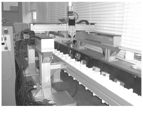
The gantry robot (Figure 1) represents an industrial tracking control problem. Mounted above a chain conveyor system, the robot is designed to collect a payload from a dispenser then place the object onto the moving conveyor. This task is fairly involved, as the robot must accurately synchronise both speed and position with the conveyor before releasing the payload. This type of operation is designed to represent an industrial system such as processed food canning, bottle filling and automotive assembly. All of
[image:3.612.318.549.130.314.2]these applications require accurate tracking control with a minimum level of error in order to maximise production rates and minimise loss of product due to faulty manufac-ture.
Fig. 1. The Gantry Robot
The robot consists of three separate axes which are mounted perpendicular to each other. The lowest horizontal axis -X moves parallel to the conveyor beneath. It is built from two subsystems, a brushless linear dc motor and an un-powered linear bearing slide. The second horizontal axis - Y has one end mounted on each component of the X -axis. TheY-axis is a single brushless linear dc motor. The vertical axis -Z, consists of a linear ball-screw stage driven by a rotary brushless dc motor. All motors are powered by performance matched dc amplifiers. Position feedback is obtained by means of optical incremental encoders. The control algorithm is implemented on a Pentium 4 PC running under the Linux operating system which is suitable for real-time control applications. The control software, signal processing hardware and instrumentation have been designed and built by the project team.
Modelling of each robot axis has been performed by means of open-loop frequency response tests. A sine-wave of known frequency and magnitude is sent to the plant. The output consists of a sine-wave of shifted phase and different magnitude. The phase shift is recorded in degrees and the magnitude difference as gain in decibels (dB). If a range of frequencies are tested, the resulting data can be used to generate a Bode plot which describes the dynamics of the plant. Using the Bode plotting rules, it is then possible to identify key features of the Bode plot such as poles, zeros and resonances, from which an approximate transfer function can be generated by hand. When deriving the transfer functions for the gantry robot, a least-mean-square algorithm was implemented to refine the approximate transfer functions and improve the match between the measured gain response and the model gain response.
process are 21st, 7th and 4th order for X, Y and Z -axes respectively. These high order models are required to accurately represent the resonant frequencies of the mechanical system. Bode plots for the measured data and the axis models can be found in [12].
The X and Y-axis, 21st and 7th order models have numerous uncontrollable and unobservable states. As all of the states must be known to implement the F-NOILC algorithm, optimal model order reduction was performed using a suitable software package to obtain a 7th order model for the X-axis and a 5th order model for the Y -axis, the highest order possible with all states controllable and observable. The transfer functions for the three models used in this paper are presented here:
• X-axis (7th order)
Gx(s) =(s+ 500.19)(s+ 4.90×10
5)
s(s+ 69.74±j459.75) × · · ·
· · · × ((ss+ 10+ 10..6999±±jj169141..62)(93)(ss+ 12+ 5.29.00±±j106j79..86)10) (12)
• Y-axis (5th order)
Gy(s) = s(s+ 78(s+ 148.54±.j20)533.34). . .
· · · ×((ss+ 213+ 49..2442±±jj526151.52).47) (13)
• Z-axis (4th order)
Gz(s) = s(s+ 989(s+ 473.06)(.s51)(+ 266s+ 199.22±.02)j157.81) (14)
Having calculated the frequency response transfer func-tions, it is then necessary to convert these into state space form. Firstly, discrete versions of the transfer functions are computed. Then suitable software is used to find the state space equivalents. The final state-space matrices for theZ -axes are presented to show the general structure which is consistent with the X andY-axes.
A =
⎡ ⎢ ⎢ ⎣
2.885 −0.758 0.342 −0.109
4 0 0 0
0 1 0 0
0 0 0.500 0
⎤ ⎥ ⎥
⎦ (15)
B = 0.0039 0 0 0 T (16)
C = 26.136 −4.484 −3.790 5.043 ×10⁻⁴ (17)
V. TEST PARAMETERS
With all axes operating simultaneously, the reference trajectories for the axes produce a three dimensional syn-chronising ‘pick and place’ action (Figure 2). The trajecto-ries produce a work rate of 30 units per minute which is equivalent to an iteration time period of 2 seconds. Using a sampling frequency of 1kHz, this generates 2000 samples per iteration.
All tests are performed in iterative learning control for-mat.
• There is a stoppage time between iterations.
• The plant is reset to known initial states before the next iteration.
• Calculation of the next ILC plant input occurs between iterations.
A two second stoppage time exists between each iteration, during which the next input to the plant is calculated. The stoppage time also allows vibrations induced in the previous iteration to die away and prevents vibrations from being propagated between iterations. Before each iteration, the axes are homed to within±30microns of a known starting location to minimise the effects of initial state error.
The plant input voltage for the first iteration is zero. Therefore the algorithm must learn to track the reference in its entirety. There is no assistance from any other form of controller.
As well as recording input voltage and axis position during each iteration, the control software also calculates the mean-square-error (mse) for position over each iteration. This is much more useful for analysing overall performance of the system and highlights whether the tracking is gener-ally improving or deteriorating. In the following sections, the mse is plotted on a logarithmic scale which improves resolution at small error values and shows up trends which may otherwise not be visible. The disadvantage of using a logarithmic scale is that the data appears to become increasingly noisy as the resolution increases.
The values Q and R for each axis were held constant for all experiments (Table I). These values were chosen because they produce good results. No attempt has been made to optimise them, or measure the effect caused by changing Q and R, this will be investigated in future work:
TABLE I
QANDRVALUES USED IN TESTING
Axis Q R
X 100I 0.01I Y 100I 0.01I Z 1000I 0.01I
In the practical implementation, the system states are es-timated by means of a tuned Full-state Luenberger observer [13].
VI. SIMULATION STUDIES
0 0.02 0.04 0.06 0.08 0.1 0.12 0.14 0.16 0
0.01 0.02
0.03 0.04 0
0.001 0.002 0.003 0.004 0.005 0.006 0.007 0.008 0.009 0.01
y−axis (m) Reference trajectory
x−axis (m)
z−axis (m)
pick
[image:5.612.66.292.74.253.2]place
Fig. 2. Three dimensional reference trajectory
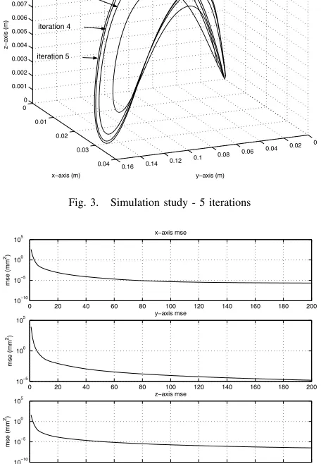
centered at the origin. Clearly, the algorithm is capable of tracking the reference trajectory (Figure 2) very well after only a few iterations. Figure 4 displays the mse tracking error for the same test up to 200 iterations, showing the high speed of convergence and the low level of error which can be achieved.
To demonstrate the saving in computation time obtained by using the F-NOILC algorithm, both variants were im-plemented at maximum rate for 100 iterations. No sample frequency restrictions were imposed on either algorithm so that the processor could implement the 100 iterations in sequence without stopping. The data for each iteration was also saved to memory, to simulate the other time requirements for a real application such as communications with the plant and data logging. The time required by the NOILC algorithm for 100 iterations was measured as 243 seconds (2.43 seconds per iteration), while the time recorded for the F-NOILC algorithm was 83 seconds (0.83 seconds per iteration). On this particular system, the F-NOILC algorithm was just less than three times faster than the NOILC.
VII. PRACTICAL IMPLEMENTATION
The F-NOILC algorithm has been implemented on the gantry robot with the models described in section IV. It is important to note that there was no difficulty implementing the high order models on the test hardware at the 1kHz sample frequency with the F-NOILC algorithm. Figure 5 shows the plant output for the first 5 iterations. Compared to the simulation study (Figure 3) the performance is very similar. This suggests that the plant models are suitably accurate.
Figure 6 shows the mse tracking error data for 5000 iterations implemented on the gantry robot. The important feature to note here is that over the 5000 trials, the system remains stable and does not diverge as many ILC algorithms tend to do [14]. This indicates that the algorithm has a good degree of robustness to non-repeating disturbances.
0 0.02 0.04 0.06 0.08 0.1 0.12 0.14 0.16 0
0.01 0.02
0.03 0.04 0
0.001 0.002 0.003 0.004 0.005 0.006 0.007 0.008 0.009 0.01
y−axis (m) Plant output
x−axis (m)
z−axis (m)
iteration 2
iteration 3
iteration 4
[image:5.612.323.547.75.257.2]iteration 5
Fig. 3. Simulation study - 5 iterations
0 20 40 60 80 100 120 140 160 180 200 10−10
10−5 100 105
x−axis mse
mse (mm
2)
0 20 40 60 80 100 120 140 160 180 200 10−5
100 105
y−axis mse
mse (mm
2)
0 20 40 60 80 100 120 140 160 180 200 10−10
10−5 100 105
z−axis mse
Iteration
mse (mm
2)
Fig. 4. Simulation study - mse 200 iterations
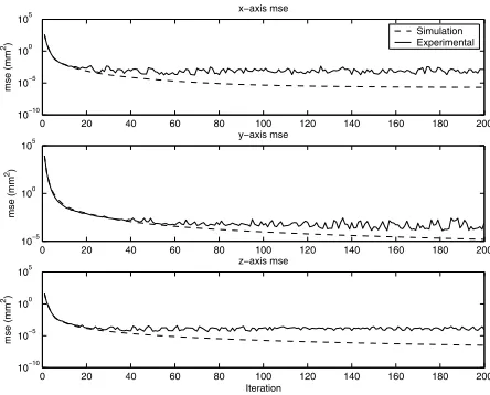
Figure 7 compares the mse plots for the practical imple-mentation and the simulation for the first 200 iterations. The mse plots are virtually identical for the first 20 -40 iterations, but then for all three axes the mse for the implementation reaches a minimum level, while the mse for the simulation continues to decrease. This is an indication that the physical plant exhibits certain non-linear effects, for example measurement quantisation and friction which the simulation does not model accurately. Measurement quantisation is particularly significant as it defines the maximum level of accuracy which the plant can achieve.
VIII. CONCLUSIONS
[image:5.612.320.548.123.452.2]0 0.02 0.04 0.06 0.08 0.1 0.12 0.14 0.16 0
0.01 0.02
0.03 0.04 0
0.001 0.002 0.003 0.004 0.005 0.006 0.007 0.008 0.009 0.01
y−axis (m) experimental plant output
x−axis (m)
z−axis (m)
iteration 2
iteration 3
iteration 4
[image:6.612.67.290.81.264.2]iteration 5
Fig. 5. Implementation - 5 iterations
0 500 1000 1500 2000 2500 3000 3500 4000 4500 5000 10−5
100 105
mse (mm
2)
x−axis mse
0 500 1000 1500 2000 2500 3000 3500 4000 4500 5000 10−5
100 105
mse (mm
2)
y−axis mse
0 500 1000 1500 2000 2500 3000 3500 4000 4500 5000 10−5
100 105
Iteration
mse (mm
2)
z−axis mse iteration 1
iteration 1
[image:6.612.67.291.302.486.2]iteration 1
Fig. 6. Implementation - mse 5000 iterations
0 20 40 60 80 100 120 140 160 180 200 10−10
10−5 100 105
x−axis mse
mse (mm
2)
0 20 40 60 80 100 120 140 160 180 200 10−5
100 105
y−axis mse
mse (mm
2)
0 20 40 60 80 100 120 140 160 180 200 10−10
10−5 100 105
z−axis mse
Iteration
mse (mm
2)
Simulation Experimental
Fig. 7. Comparison - simulation and experimental mse 200 iterations
tracking accuracy in a minimal number of repetitions and should therefore be very attractive to industry.
IX. FUTURE WORK
Future work will involve three components. Firstly, test-ing the effect of Q and R on the convergence rate and algorithm robustness. Secondly, investigating the robustness by using simpler and less accurate models. Finally, in most applications, many of the elements of the F-NOILC matrices are redundant because they are either zero, or replicated many times. To reduce the memory requirements posed by the F-NOILC, it should be possible to compact these matrices into a more efficient form. The F-NOILC would then provide significantly increased computation speed at little cost to memory requirements and would therefore be particularly suited to industrial applications.
REFERENCES
[1] S. Kawamura, F. Miyazaki, and S. Arimoto, “Applications of learning method for dynamic control of robot manipulators,” inProceedings of the 24th Conference on Decision and Control, Ft. Lauderdale, FL, December 1985, pp. 1381–1386.
[2] N. Amann, D. Owens, and E. Rogers, “Iterative learning control using optimal feedback and feedforward actions,”International Journal of Control, vol. 65, no. 2, pp. 277–293, 1996.
[3] S. Arimoto, S. Kawamura, and F. Miyazaki, “Bettering operation of dynamic systems by learning : A new control theory for servomech-anism or mechatronic systems,” inProceedings of 23rd Conference on Decision and Control, Las Vegas, NV, December 1984, pp. 1064– 1069.
[4] ——, “Bettering operation of robots by learning,”Journal of Robotic Systems, vol. 1, pp. 123–140, 1984.
[5] J.-X. Xu, B. Viswanathan, and Z. Qu, “Robust learning control for robotic manipulators with an extension to a class of non-linear systems,”International Journal of Control, vol. 73, no. 10, pp. 858– 870, 2000.
[6] J.-X. Xu and B. Viswanathan, “Adaptive robust iterative learning control with dead zone scheme,” Automatica, vol. 36, pp. 91–99, 2000.
[7] N. Amann, D. Owens, and E. Rogers, “Predictive optimal iterative learning control,”International Journal of Control, vol. 69, no. 2, pp. 203–226, 1998.
[8] K. Dutton, S. Thompson, and B. Barraclough,The art of control engineering. Addison-Wesley, 1998.
[9] J. Machado and A. Galhano, “Benchmarking computer systems for robot control,”IEEE Transactions on Education, vol. 38, no. 3, pp. 205–210, August 1995.
[10] N. Amann, D. Owens, and E. Rogers, “Iterative learning control for discrete-time systems with exponential rate of convergence,”IEE Proceedings on Control Theory Applications, vol. 143, no. 2, pp. 217–224, March 1996.
[11] T. Al-Towaim, A. Barton, P. Lewin, E. Rogers, and D. Owens, “Iterative learning control — 2d control systems from theory to application,”International Journal of Control, 2004, in press. [12] J. Ratcliffe, T. Harte, J. Hätönen, P. Lewin, E. Rogers, and D. Owens,
“Practical implementation of a model inverse iterative learning con-troller,” inProceedings of the IFAC Workshop on Periodic Control Systems (PSYCO 04), 2004.
[13] D. Luenberger, “An introduction to observers,”IEEE Transaction on Automatic Control, vol. 16, no. 6, pp. 596–602, December 1971. [14] R. Longman, “Iterative learning control and repetitive control for
[image:6.612.67.289.534.713.2]