BLOCK-TOEPLITZ/HANKEL STRUCTURED TOTAL LEAST SQUARES∗
IVAN MARKOVSKY†, SABINE VAN HUFFEL†,AND RIK PINTELON‡
Abstract. A structured total least squares problem is considered in which the extended data matrix is partitioned into blocks and each of the blocks is block-Toeplitz/Hankel structured, unstruc-tured, or exact. An equivalent optimization problem is derived and its properties are established. The special structure of the equivalent problem enables us to improve the computational efficiency of the numerical solution methods. By exploiting the structure, the computational complexity of the algorithms (local optimization methods) per iteration is linear in the sample size. Application of the method for system identification and for model reduction is illustrated by simulation examples.
Key words. parameter estimation, total least squares, structured total least squares, system identification, model reduction
AMS subject classifications. 15A06, 62J12, 37M10
DOI.10.1137/S0895479803434902
1. Introduction. Thetotal least squares(TLS) problem
min
ΔA,ΔB,X
ΔA ΔB2F subject to (A−ΔA)X =B−ΔB,
(1.1)
where A ∈ Rm×n, B ∈ Rm×d, C := [A B] is the data matrix, and X ∈ Rn×d is the parameter of interest, proved to be a useful parameter estimation technique. It became especially popular since the early eighties due to the development [8] of reliable solution methods based on singular value decomposition. The same technique is known in the system identification literature as the Koopmans–Levin method [12] and in the statistical literature as orthogonal regression [7]. For a comprehensive introduction to the theory, algorithms, and applications of the TLS method, see [25]. With the increased interest in the TLS technique, more and more researchers started to apply it in various applications. In some cases, however, important assump-tions of the method are not satisfied, which resulted in the development of appropri-ate extensions of the original TLS method. We mention the mixed LS-TLS method
∗Received by the editors September 15, 2003; accepted for publication (in revised form) by L. Eld´en June 30, 2004; published electronically May 6, 2005. This research was supported by Research Council K. U. Leuven through grants GOA-Mefisto 666, IDO/99/003, and IDO/02/009 (predictive computer models for medical classification problems using patient data and expert knowledge) and several Ph.D./postdoctorate and fellow grants; the Flemish Government, FWO, through Ph.D./postdoctorate grants, projects, and grants G.0200.00 (damage detection in composites by optical fibers), G.0078.01 (structured matrices), G.0407.02 (support vector machines), G.0269.02 (magnetic resonance spectroscopic imaging), and G.0270.02 (nonlinear Lp approximation); research communities (ICCoS, ANMMM); the AWI under the Bil. Int. Collaboration Hungary/Poland; the IWT through Ph.D. grants; the Belgian Federal Government, DWTC (grants IUAP IV-02 (1996– 2001) and IUAP V-22 (2002–2006): Dynamical Systems and Control: Computation, Identification & Modelling); the EU through NICONET, INTERPRET, PDT-COIL, MRS/MRI signal processing (TMR); and contract research/agreements (Data4s, IPCOS).
http://www.siam.org/journals/simax/26-4/43490.html
†ESAT-SCD (SISTA), Katholieke Universiteit Leuven, Kasteelpark Arenberg 10, B-3001 Leuven-Heverlee, Belgium ([email protected], Sabine.VanHuff[email protected]). The first author was supported by a K.U. Leuven doctoral scholarship.
‡Department ELEC, Vrije Universiteit Brussel, Pleinlaan 2, B-1050 Brussels, Belgium (Rik. [email protected]).
[25, sect. 3.5], where some of the columns of A are exact (noise free), and the so-called generalized total least squares method [24], where the cost function of TLS problem (1.1) is generalized to ΔA ΔBV2
F, with V ≥0. The latest
develop-ments in the field are collected in the proceedings books [22, 23].
In the early nineties, a powerful generalization of the TLS method was put for-ward [1, 4, 20]. The so-calledstructured total least squares (STLS) problem,
min
ΔA,ΔB,X
ΔA ΔB2F subject to (A−ΔA)X =B−ΔB and
ΔA ΔB has the same structure as A B,
defined in the same way as the TLS problem (1.1) but with the additional structure constraint, includes as special cases many of the presently known TLS variations. The structure occurs naturally in, e.g., applications dealing with discrete-time dynamic phenomena [6], where the Hankel and Toeplitz matrices are fundamental.
Although the STLS problem is very general, it is still not widely accepted due to the lack of reliable solution methods for its computation, the main difficulty being that, as an optimization problem, it is nonconvex and there is no guarantee that a global minimum point will be found. Still, under certain conditions [10] for highly overdetermined systems (mnd) the solution of the problem is unique and the main difficulty—the presence of multiple local minima—tends to disappear for large sample sizes (i.e., for m→ ∞). In addition, due to the consistency results of [10], such an assumption guarantees accurate estimation and makes the problem meaningful from a statistical point of view.
However, the currently used numerical algorithms for solving the STLS problem can hardly deal with large sample sizes. The original methods of [1, 4, 20] have computational costs that increase quadratically or even cubically as a function ofm. In [11, 17], methods with computational cost linear in m are developed using the generalized Schur algorithm. These methods, however, are developed for a particular structure of the data matrixC (in [11]C is Hankel, and in [17]A∈Rm×n is Toeplitz andB∈Rm×1is unstructured) and modifications for other structures are nontrivial.
In [13], based on the insight from [10], we have proposed a new approach with computational cost linear inmand dealing with a flexible structure specification. The data matrixC can be partitioned into blocksC=C(1) · · · C(q), where each of the
blocksC(l), forl= 1, . . . , q, is Hankel, Toeplitz, unstructured, or exact.
In this paper, we consider an extension of the results of [13] to the case of block-Hankel and block-Toeplitz structured matrices. Thus the data matrix is now a block matrix, of which the blocks are themselves structured with one of the four possible structures: block-Hankel, block-Toeplitz, unstructured, or exact. The need for such an extension comes from applications dealing with multi-input and/or multi-output dynamical systems. The proposed algorithms are implemented in C (see [15]), and the software is available.
Standard notation used in the paper is as follows: R for the set of the real numbers,Nfor the set of the natural numbers, · for the Euclidean norm, and · F
for the Frobenius norm. The operator that vectorizes columnwise a matrix is denoted by vec(·), the expectation operator by E, and the covariance matrix of a random vector by cov(·). The pseudoinverse of a matrixAis denoted byA†.
2. The STLS problem. In this section, we define the STLS problem, con-sidered in the paper, and derive an equivalent optimization problem. Consider a functionS :Rnp→Rm×(n+d)that defines the structure of the data as follows: a
such that C = S(p). The vector p is called a parameter vector for the structured matrixC.
Problem 2.1 (STLS problem). Given a data vector p ∈ Rnp and a structure
specification S:Rnp →Rm×(n+d), solve the optimization problem
min X,Δp
Δp2 subject to S(p−Δp)
X −Id
= 0.
(2.1)
The interpretation of (2.1) is the following: Find the smallest correction Δp, measured in 2-norm, that makes the structured matrixS(p−Δp) rank deficient with rank at mostn. Define
Xext :=
X −Id
, and A B:=C:=S(p), whereA∈Rm×n andB∈Rm×d.
CXext= 0 is shorthand notation for the structured system of equations AX=B.
The STLS problem is said to beaffine structured if the functionS is affine, i.e.,
S(p) =S0+
np
i=1
Sipi for allp∈Rnp and for someSi, i= 1, . . . , np. (2.2)
In an affine STLS problem, the constraintS(p−Δp)Xext= 0 becomes bilinear in the
decision variablesX and Δp.
Lemma 2.2. Let S:Rnp→Rm×(n+d) be an affine function. Then S(p−Δp)Xext= 0 ⇐⇒ G(X)Δp=r(X),
where
G(X) :=vec(S1Xext) · · · vec
(SnpXext) ∈R
md×np
(2.3)
and
r(X) := vecS(p)Xext ∈Rmd.
Proof.
S(p−Δp)Xext= 0 ⇐⇒
np
i=1
SiΔpiXext=S(p)Xext
⇐⇒
np
i=1
vec(SiXext) Δpi= vec
S(p)Xext
⇐⇒ G(X)Δp=r(X).
Using Lemma 2.2, we rewrite the affine STLS problem as follows:
min X
min
Δp
Δp2 subject to G(X)Δp=r(X)
.
(2.4)
Theorem 2.3 (equivalent optimization problem for affine STLS).Assuming that np≥md, the affine STLS problem(2.4)is equivalent to
min
X f0(X), wheref0(X) :=r
(X)Γ†(X)r(X) and Γ(X) :=G(X)G(X). (2.5)
Proof. Under the assumptionnp≥md, the inner minimization problem of (2.4) is a least norm problem. Its minimum point (as a function ofX) is
Δpmin(X) =G(X)
G(X)G(X) †r(X),
so that
f0(X) = Δpmin(X)Δpmin(X) =r(X)
G(X)G(X) †r(X) =r(X)Γ†(X)r(X).
The significance of Theorem 2.3 is that the constraint and the decision variable Δp
in problem (2.4) are eliminated. Note that typically the number of elementsndinX
is much smaller than the number of elements np in the correction Δp. Thus the reduction in the complexity is significant.
The equivalent optimization problem (2.5) is a nonlinear least squares problem, so that classical optimization methods can be used for its solution. The optimization methods require a cost function and first derivative evaluation. In order to evaluate the cost functionf0for a given value of the argumentX, we need to form the weight
matrix Γ(X) and to solve the system of equations Γ(X)y(X) =r(X). This straight-forward implementation requiresO(m3) floating point operation (flops). For largem
(the applications that we aim at) this computational complexity becomes prohibitive. It turns out, however, that for a special case of affine structures S, the weight matrix Γ(X) is nonsingular and has a block-Toeplitz and block-banded structure, which can be exploited for efficient cost function and first derivative evaluations. The set of structures ofS, for which we establish the special properties of Γ(X), is
S(p) =C(1) · · · C(q) for allp∈Rnp, where C(l), forl= 1, . . . , q, is
block-Toeplitz, block-Hankel, exact, or unstructured and all block-Toeplitz/Hankel structured blocksC(l)
have equal row dimensionK of the blocks. (2.6)
Assumption (2.6) says thatS(p) is composed of blocks, each of which is block-Toeplitz, block-Hankel, exact, or unstructured. A blockC(l)that is exact is not modified in the solution ˆC:=S(p−Δp), i.e., ˆC(l)=C(l). Assumption 2.6 is the essential structural
assumption that we impose on problem (2.1). As shown in section 6, it is fairly general and covers many applications.
Example 1. Consider the block-Toeplitz matrix
C= ⎡ ⎢ ⎢ ⎢ ⎢ ⎢ ⎢ ⎢ ⎢ ⎢ ⎣
5 6
3 4
1 2
7 8
5 6
3 4
9 10
7 8
5 6
with row dimension of the blockK = 2. Next we specify the matricesSi that define via (2.2) an affine functionS, such that C =S(p) for a certain parameter vector p. Let == be an elementwise comparison operator. Acting on matrices of the same size, it gives as a result a matrix with the same size as the arguments, of which the (i, j)th element is 1 if the corresponding elements of the arguments are equal, and 0 otherwise. (Think of Matlab’s == operator.) Let E be the 6×3 matrix with all
elements equal to 1 and defineS0:= 06×3andSi:= (C==iE) fori= 1, . . . ,10. We have
C=
10
i=1
Sii=S0+ 10
i=1
Sipi=:S(p), withp=
1 2 · · · 10.
The matrixCconsidered in the example is special; it allowed us to easily write down a corresponding affine function S. Clearly with the constructedS, any 6×3 block-Toeplitz matrixCwith row dimension of the blockK= 2 can be written asC=S(p) for certainp∈R10.
We will use the notation nl for the number of block columns of the block C(l).
For unstructured and exact blocks,nl:= 1.
3. Properties of the weight matrix Γ. For the evaluation of the cost func-tionf0 of the equivalent optimization problem (2.5), we have to solve the system of
equations Γ(X)y(X) =r(X), where Γ(X)∈Rmd×np with both mand n
p large. In this section, we investigate the structure of the matrix Γ(X). Occasionally we drop the explicit dependence ofrand Γ onX.
Theorem 3.1 (structure of the weight matrix Γ). Consider the equivalent
op-timization problem (2.5) from Theorem 2.3. If, in addition to the assumptions of Theorem 2.3, the structure S is such that (2.6) holds, then the weight matrix Γ(X) has the block-banded Toeplitz structure
Γ(X) = ⎡ ⎢ ⎢ ⎢ ⎢ ⎢ ⎢ ⎢ ⎢ ⎢ ⎢ ⎣
Γ0 Γ1 · · · Γs 0
Γ1 . .. . .. . .. . ..
..
. . .. . .. . .. . .. Γs Γs . .. . .. . .. . .. ...
. .. . .. . .. . .. Γ
1
0 Γs · · · Γ1 Γ0
⎤ ⎥ ⎥ ⎥ ⎥ ⎥ ⎥ ⎥ ⎥ ⎥ ⎥ ⎦
∈Rmd×md, (3.1)
whereΓk∈RdK×dK, fork= 0,1, . . . , s, ands= maxl=1,...,q(nl−1), wherenl is the number of block columns in the blockC(l) of the data matrix S(p).
The proof is developed in a series of lemmas. First we reduce the original problem with multiple blocks C(l) (see (2.6)) to three independent problems—one for the
unstructured case, one for the block-Hankel case, and one for the block-Toeplitz case.
Lemma 3.2. Consider a structure specification of the form
S(p) =S(1)(p(1)) · · · S(q)(p(q)), p(l)∈Rn(pl), q
l=1
n(pl)=:np,
wherep =:p(1) · · · p(q)andS(p(l)) :=S(l) 0 +
n(l) p
i=1S (l)
i p
(l)
i for allp(l)∈R n(l)
l= 1, . . . , q. Then
Γ(X) = q
l=1
Γ(l)(X),
(3.2)
whereΓ(l):=G(l)G(l),G(l):= [vec((S(l) 1 X
(l)
ext)) · · · vec((S (l)
n(pl)X
(l)
ext))], and
Xext=: ⎡ ⎢ ⎢ ⎣
Xext(1)
.. .
Xext(q)
⎤ ⎥ ⎥
⎦, with Xext(l) ∈Rnl×d, n
l:= coldim(C(l)), q
l=1
nl=n+d.
Proof. The result is a refinement of Lemma 2.2. Let Δp=:Δp(1) · · · Δp(q),
where Δp(l)∈Rnp(l) forl= 1, . . . , q. We have
S(p−Δp)Xext= 0 ⇐⇒
q
l=1
S(l)(p(l)−Δp(l))X(l) ext= 0
⇐⇒
q
l=1
np
i=1
Si(l)Δp(il)Xext(l) =S(p)Xext
⇐⇒
q
l=1
G(l)Δp(l)=r(X)
⇐⇒ G(1) · · · G(q)
G(X)
Δp=r(X),
so that Γ =GG =ql=1G(l)G(l)=q
l=1Γ (l).
Next we establish the structure of Γ for an STLS problem with an unstructured data matrix.
Lemma 3.3. Let
S(p) := ⎡ ⎢ ⎢ ⎢ ⎣
p1 p2 · · · pn+d
pn+d+1 pn+d+2 · · · p2(n+d)
..
. ... ...
p(m−1)(n+d)+1 p(m−1)(n+d)+2 · · · pm(n+d)
⎤ ⎥ ⎥ ⎥ ⎦∈R
m×(n+d);
then
Γ =Im⊗(Xext Xext);
(3.3)
i.e., the matrixΓ has the structure (3.1)withs= 0 andΓ0=IK⊗(Xext Xext).
Proof. We have
S(p−Δp)Xext= 0 ⇐⇒ vec
Xext S(Δp) = vecS(p)Xext
⇐⇒ (Im⊗Xext )
G(X)
vecS(Δp)
Δp
=r(X).
Therefore, Γ =GG= (Im⊗Xext )(Im⊗Xext )=Im⊗(Xext Xext).
Lemma 3.4. Let
S(p) := ⎡ ⎢ ⎢ ⎢ ⎣
C1 C2 · · · Cn
C2 C3 · · · Cn+1
..
. ... ...
Cm Cm+1 · · · Cm+n−1
⎤ ⎥ ⎥ ⎥ ⎦∈R
m×(n+d),
n:= n+d
L ,
m:= m
K,
whereCi are K×Lunstructured blocks, parameterized byp(i)∈RKL as follows:
Ci := ⎡ ⎢ ⎢ ⎢ ⎢ ⎣
p(1i) p(2i) · · · p(Li) pL(i+1) p(Li+2) · · · p(2iL)
..
. ... ...
p((iK)−1)L+1 p((Ki)−1)L+2 · · · p(KLi)
⎤ ⎥ ⎥ ⎥ ⎥ ⎦∈R
K×L.
Define a partitioning ofXextas follows: Xext =:X1 · · · Xn
, whereXj∈Rd×L. ThenΓ has the block-banded Toeplitz structure(3.1)withs=n−1 and with
Γk = n−k
j=1
XjXj+k, where Xk:=IK⊗Xk. (3.4)
Proof. Define the residualR:=S(Δp)Xextand the partitioningR=:
R1· · ·Rm
, whereR1∈Rd×K. Let ΔC:=S(Δp), with blocks ΔCi. We have
S(p−Δp)Xext = 0 ⇐⇒ S(Δp)Xext=S(p)Xext
⇐⇒ ⎡ ⎢ ⎢ ⎢ ⎣
X1 X2 · · · Xn
X1 X2 · · · Xn . .. . .. . ..
X1 X2 · · · Xn ⎤ ⎥ ⎥ ⎥ ⎦ ⎡ ⎢ ⎢ ⎢ ⎣
ΔC1
ΔC2
.. . ΔCm+n−1
⎤ ⎥ ⎥ ⎥ ⎦= ⎡ ⎢ ⎢ ⎢ ⎣
R1 R2
.. .
Rm ⎤ ⎥ ⎥ ⎥ ⎦ ⇐⇒ ⎡ ⎢ ⎢ ⎢ ⎣
X1 X2 · · · Xn
X1 X2 · · · Xn
. .. . .. . .. X1 X2 · · · Xn
⎤ ⎥ ⎥ ⎥ ⎦
G(X)
⎡ ⎢ ⎢ ⎢ ⎣
vec(ΔC1)
vec(ΔC2) .. . vec(ΔCm+n−1)
⎤ ⎥ ⎥ ⎥ ⎦ Δp = ⎡ ⎢ ⎢ ⎢ ⎣
vec(R1)
vec(R2) .. . vec(Rm)
⎤ ⎥ ⎥ ⎥ ⎦
r(X) .
Therefore, Γ =GG has the structure (3.1), with Γk’s given by (3.4).
The derivation of the Γ matrix for an STLS problem with block-Toeplitz data matrix is analogous to the one for an STLS problem with block-Hankel data matrix. We state the result in the next lemma.
Lemma 3.5. Let
S(p) := ⎡ ⎢ ⎢ ⎢ ⎣
Cn Cn−1 · · · C1
Cn+1 Cn · · · C2
..
. ... ...
Cm+n−1 Cm+n−2 · · · Cm ⎤ ⎥ ⎥ ⎥ ⎦∈R
with the blocks Ci defined as in Lemma 3.4. Then Γ has the block-banded Toeplitz structure(3.1)with s=n−1 and with
Γk= n
j=k+1
XjXj−k.
(3.5)
Proof. Following the same derivation as in the proof of Lemma 3.4, we find that
G= ⎡ ⎢ ⎢ ⎢ ⎣
Xn Xn−1 · · · X1
Xn Xn−1 · · · X1
. .. . .. . .. Xn Xn−1 · · · X1
⎤ ⎥ ⎥ ⎥ ⎦.
Therefore, Γ =GG has the structure (3.1), with Γk’s given by (3.5).
Proof of Theorem3.1. Lemmas 3.2–3.5 show that the weight matrix Γ for the origi-nal problem has the block-banded Toeplitz structure (3.1) withs= maxl=1,...,q(nl−1), wherenlis the number of block columns in thelth block of the data matrix.
Apart from revealing the structure of Γ, the proof of Theorem 3.1 gives an algo-rithm for the construction of the blocks Γ0,. . . ,Γs that define Γ:
Γk = q
l=1
Γ(kl), where Γ(kl)= ⎧ ⎪ ⎪ ⎪ ⎨ ⎪ ⎪ ⎪ ⎩
nl
j=k+1X (l)
j X
(l)
j−k ifC
(l)is block-Toeplitz,
nl−k
j=1 X (l)
j X
(l)
j+k ifC(l)is block-Hankel, 0dK ifC(l)is exact, or
δkIK⊗(X
(l) ext X
(l)
ext) ifC(l)is unstructured,
(3.6)
whereδis the Kronecker delta function: δ0= 1 and δk = 0 fork= 0.
Corollary 3.6 (positive definiteness of the weight matrix Γ). Assume that the
structure ofS is given by(2.6)with the block C(q) being block-Toeplitz, block-Hankel, or unstructured and having at least d columns. Then the matrix Γ(X) is positive definite for allX ∈Rn×d.
Proof. We will show that Γ(q)(X) >0 for all X ∈ Rn×d. From (3.2), it follows that Γ has the same property. By the assumption col dim(C(q))≥d, it follows that Xext(q)= [−∗Id], where the∗denotes a block (possibly empty) depending onX. In the
unstructured case, Γ(q) = I
m⊗(X
(q) ext X
(q)
ext); see (3.6). But rank(X (q) ext X
(q) ext) = d,
so that Γ(q)is nonsingular. In the block-Hankel/Toeplitz case,G(q) is block-Toeplitz
and block-banded; see Lemmas 3.4 and 3.5. One can verify by inspection that in-dependent of X, G(q)(X) has full row rank due to its row echelon form. Then
Γ(q)=G(q)G(q)>0.
The positive definiteness of Γ is studied in a statistical setting in [10, sect. 4], where more general conditions are given. The restriction of (2.6) that ensures Γ>0 is fairly minor, so that in what follows we will consider STLS problems of this type and replace the pseudoinverse in (2.5) with the inverse.
In the next section, we give an interpretation of Theorem 3.1 from a statistical point of view, and in section 5 we consider in more detail the algorithmic side of the problem.
4. Stochastic interpretation. Our work on the STLS problem has its origin in the field of estimation theory. A linear multivariate errors-in-variables (EIV) model is defined as follows:
AX≈B, where A= ¯A+ ˜A, B= ¯B+ ˜B, and A¯X¯ = ¯B.
The observations A and B are obtained from (nonstochastic) true values A¯ and ¯B
withmeasurement errors A˜ and ˜B that are zero mean random matrices. Define the extended matrix ˜C := A˜ B˜ and the vector ˜c := vec( ˜C) of the measurement errors. It is well known (see [25, Chap. 8]) that the TLS problem (1.1) provides a consistent estimator for the true value of the parameter ¯X in the EIV model (4.1) if cov(˜c) =σ2I (and additional technical conditions are satisfied). If, in addition to cov(˜c) =σ2I, ˜c is normally distributed, i.e., ˜c∼N(0, σ2I), then the solution ˆXtlsof
the TLS problem is the maximum likelihood estimate of ¯X.
The EIV model (4.1) is called thestructured errors-in-variables model if the ob-served dataC and the true value ¯C := A¯ B¯ have a structure defined by a func-tionS. Therefore,
C=S(p) and C¯ =S(¯p),
where ¯p∈Rnp is a (nonstochastic) true value of the parameterp. As a consequence
the matrix of measurement errors is also structured. LetS be affine (2.2). Then
˜
C= np
i=1
Sip˜i and p= ¯p+ ˜p,
where the random vector ˜p represents the measurement error on the structure pa-rameter ¯p. In [10], it is proven that the STLS problem (2.1) provides a consistent estimator for the true value of the parameter ¯X if cov(˜p) = σ2I (and additional
technical conditions are satisfied). If ˜p∼N(0, σ2I), then a solution ˆX of the STLS
problem is a maximum likelihood estimate of ¯X.
Let ˜r(X) := vecS(˜p)Xext be the random part of the residualr. In the stochastic
setting, the weight matrix Γ is up to the scale factor σ2 equal to the covariance
matrixVr˜:= cov(˜r). Indeed, ˜r=Gp˜, so that
Vr˜:=E˜r˜r=GE(˜pp˜)G =σ2GG=σ2Γ.
Next we show that the structure of Γ is in a one-to-one correspondence with the structure of V˜c := cov(˜c). Let Γij ∈ RdK×dK be the (i, j)th block of Γ and let Vc,ij˜ ∈ R(n+d)K×(n+d)K be the (i, j)th block of V˜c. Define also the following partitionings of the vectors ˜rand ˜c:
˜
r=: ⎡ ⎢ ⎣ ˜ r1
.. . ˜rm
⎤ ⎥
⎦, ˜ri∈RdK and c˜=: ⎡ ⎢ ⎣ ˜ c1
.. . ˜ cm
⎤ ⎥
⎦, ˜ci∈R(n+d)K,
wherem:=m/K. Usingri=Xextci, where Xext:= (IK⊗Xext ), we have σ2Γij =E˜ri˜rj =XextE(˜ci˜cj)Xext =XextV˜c,ijXext.
(4.2)
The one-to-one relation between the structures of Γ andV˜callows us to relate the structural properties of Γ, established in Theorem 3.1, with statistical properties of the measurement errors. Define stationarity ands-dependence of a centered sequence of random vectors ˜c:={˜c1,˜c2, . . .}, ˜ci∈R(n+d)K as follows:
• ˜cis s-dependentif the covariance matrix Vc˜is block-banded with block size
(n+d)K×(n+d)K and block bandwidth 2s+ 1.
The sequence of measurement errors ˜cbeing stationary ands-dependent corresponds to Γ being block-Toeplitz and block-banded.
The statistical setting gives an insight into the relation between the structure of the weight matrix Γ and the structure of the data matrix C. It can be verified that the structure specification (2.6) implies stationarity ands-dependence for ˜c. This indicates an alternative (statistical) proof of Theorem 3.1; see the technical report [14]. The blocks of Γ are quadratic functions of X, Γij(X) =XextW˜c,ijXext, where W˜c,ij :=V˜c,ij/σ2; see (4.2). Moreover, by Theorem 3.1, we have that under assump-tion (2.6),W˜c,ij=W˜c,|i−j|for certain matricesW˜c,k,k= 1, . . . ,m, andW˜c,ij= 0 for
|i−j|> s, wheresis defined in Theorem 3.1. Therefore,
Γk(X) =XextW˜c,kXext fork= 0,1, . . . , s, where W˜c,k := 1
σ2V˜c,k.
In (3.6) we show how the matrices {Γk}s
k=0 can be determined from the structure
specification (2.6). Similar expressions can be written for the matrices{W˜c,k}sk=0.
In the computational algorithm described in section 5, we use the partitioning of the matrix Γ into blocks of sized×d. Let Γij ∈Rd×d be the (i, j)th block of Γ and letVc,ij˜ ∈R(n+d)×(n+d)be the (i, j)th block ofV˜c. Define the following partitionings
of the vectors ˜rand ˜c:
˜
r=: ⎡ ⎢ ⎣ ˜
r1
.. . ˜
rm ⎤ ⎥
⎦, ri∈Rd and ˜c=: ⎡ ⎢ ⎣ ˜
c1
.. . ˜
cm ⎤ ⎥
⎦, ci∈Rn+d.
Usingri=Xext ci, we have
Γij = 1
σ2Er˜i˜rj= 1
σ2Xext E(˜ci˜cj)Xext =
1
σ2Xext V˜c,ijXext=:Xext Wc,ij˜ Xext.
5. Efficient cost function and first derivative evaluation. We consider an efficient numerical method for solving the STLS problem (2.1) by applying standard local optimization algorithms to the equivalent problem (2.5). With this approach, the main computational effort is in the cost function and its first derivative evaluation. First, we describe the evaluation of the cost function: givenX, computef0(X).
For given X, and with {Γk}sk=0 constructed as described in the proof of Theo-rem 3.1, the weight matrix Γ(X) is specified. Then from the solution of the sys-tem Γ(X)yr(X) =r(X), the cost function is found asf0(X) =r(X)yr(X).
The properties of Γ(X) can be exploited in the solution of the system Γyr=r. The subroutineMB02GDfrom the SLICOT library [2] exploits both the block-Toeplitz and the banded structure to compute a Cholesky factor of Γ in O((dK)2sm) flops.
In combination with the LAPACK subroutine DPBTRSthat solves block-banded tri-angular systems of equations, the cost function is evaluated in O(m) flops. Thus an algorithm for local optimization that uses only cost function evaluations has com-putational complexity O(m) flops per iteration, because the computations needed internally for the optimization algorithm do not depend onm.
Next, we describe the evaluation of the derivative. The derivative of the cost functionf0 is (see the appendix)
f0(X) = 2 m
i,j=1
ajri (X)Mij(X)−2 m
i,j=1
I 0W˜c,ij
X −I
Nji(X),
whereA =:a1 · · · am
, withai∈Rn,
M(X) := Γ−1(X), N(X) := Γ−1(X)r(X)r(X)Γ−1(X),
andMij∈Rd×d,Nij∈Rd×d are the (i, j)th blocks ofM andN, respectively. Consider the two partitionings ofyr∈Rmd,
yr=: ⎡ ⎢ ⎣
yr,1
.. .
yr,m ⎤ ⎥
⎦, yr,i∈Rd and yr=: ⎡ ⎢ ⎣
yr,1
.. . yr,m
⎤ ⎥
⎦, yr,i∈RdK,
(5.2)
wherem:=m/K. The first sum in (5.1) becomes
m
i,j=1
ajri Mij=AYr, where Yr :=
yr,1 · · · yr,m
.
(5.3)
Define the sequence of matrices
Nk := m−k
i=1
yr,i+kyr,i, Nk=N−k, k= 0, . . . , s.
The second sum in (5.1) can be written as
m
i,j=1
I 0W˜c,ij
X −I
Nji= s
k=−s K
i,j=1
(W˜a,k,ijX−Wa˜b,k,ij˜ )Nk,ij,
whereW˜c,k,ij∈R(n+d)×(n+d)is the (i, j)th block ofW˜c,k∈RK(n+d)×K(n+d),W˜a,k,ij∈ Rn×n andW
˜
ab,k,ij˜ ∈R
n×d are defined as blocks ofW
˜
c,k,ij as
W˜c,k,ij =:
Wa,k,ij˜ W˜a˜b,k,ij
W˜b˜a,k,ij Wb,k,ij˜
,
andNk,ij∈Rd×d is the (i, j)th block ofNk∈RdK×dK.
Thus the evaluation of the derivativef0(X) uses the solution of Γyr=r, already computed for the cost function evaluation and additional operations of O(m) flops. The steps described above are summarized in Algorithm 1.
Algorithm 1. Cost function and first derivative evaluation.
1: Input: A,B,X, {W˜c,k}sk=0.
2: Γk= (IK⊗Xext )W˜c,k(IK⊗Xext ) fork= 0,1, . . . , s, 3: r= vec(AX−B) ,
4: solve (viaMB02GDandDPBTRS) Γyr=r, where Γ is given in (3.1),
5: f0=ryr.
6: If only the cost function evaluation is required, outputf0 and stop. 7: Nk=mi=1−kyr,i+kyr,i fork= 0,1, . . . , s, whereyi is defined in (5.2).
8: f0 = 2AYr−2 s
k=−s K
i,j=1(W˜a,k,ijX−Wa˜b,k,ij˜ )Nk,ij, where Yr is defined in (5.3).
The flops per step for Algorithm 1 are as follows: 2. (n+d)(n+ 2d)dK3.
3. m(n+ 1)d. 4. msd2K2.
5. md.
7. msd2K−s(s+ 1)d2K2/2.
8. mnd+ (2s+ 1)(nd+n+ 1)dK2.
Thus in total O(md(sdK2+n) +n2dK3+ 3nd2K3+ 2d3K3+ 2snd2K2) flops are
required for cost function and first derivative evaluation. Note that the flop counts depend on the structure throughs.
Using the computation of the cost function and its first derivative, as outlined above, we can apply the BFGS (Broyden, Fletcher, Goldfarb, and Shanno) quasi-Newton method. A more efficient alternative, however, is to apply a nonlinear least squares optimization algorithm, such as the Levenberg–Marquardt algorithm. Let Γ = UU be the Cholesky factorization of Γ. Then f = FF, with F := U−1r.
(Note that the evaluation of F(X) is cheaper than that of f(X).) We do not know an analytic expression for the Jacobian matrixJ(X) = [∂Fi/∂xj], but instead we use the so-called pseudo-JacobianJ+ proposed in [9]. The evaluation ofJ+ can be done
efficiently, using the approach described above forf(X).
Moreover, by using the nonlinear least squares approach and the pseudo-Jacobian
J+, we have as a byproduct of the optimization algorithm an estimate of the covariance
matrix Vxˆ = E
vec( ˆX)vec( ˆX) . As shown in [19, Chap. 17.4.7, eqns. (17)–(35)],
Vˆx≈
J+( ˆX)J+( ˆX) − 1
. UsingVxˆ, we can compute statistical confidence bounds for
the estimate ˆX.
6. Applications and simulation examples. Under assumption (2.6), the specification of S is given by K and the array D ∈ {(T,H,U,E)×N×N}q that de-scribes the structure of the blocks{C(l)}q
l=1;Dl specifies the block C(l)by giving its typeDl(1) (T= block-Toeplitz,H= block-Hankel,U= unstructured, andE= exact), the number of columnsnl=Dl(2), and, for block-Toeplitz/Hankel blocks, the column dimensionDl(3) of the block. The following well-known problems are special cases of the block-Toeplitz/Hankel STLS problem of this paper for particular choices of the structure descriptionD. (If not specified, K and the third element of Dl are equal to one.)
1. Least squares problem: AX ≈B, A ∈ Rm×n exact, B ∈ Rm×d noisy and unstructured is achieved byD= [[En],[Ud]].
2. TLS problem: AX ≈B, C = [A B]∈ Rm×(n+d) noisy and unstructured is
achieved byD= [Un+d].
3. Data least squares problem [3]: AX≈B,A∈Rm×n noisy and unstructured, andB∈Rm×d exact is achieved by D= [[Un],[Ed]].
4. Mixed LS-TLS problem[25, sect. 3.5]: AX≈B,A= [AnoisyAexact],Anoisy∈
Rm×n1 andB ∈Rm×d noisy and unstructured,A
exact∈Rm×n2 exact is achieved by
D= [[Un1],[En2],[Ud]].
5. Hankel low-rank approximation problem [4, sect. 4.5], [21]:
min
Δp Δp
2 subject to H(p−Δp) has given rankn,
(6.1)
where H is a mapping from the parameter spaceRnp to the set of them×(n+d)
H(ˆp) X −I
= 0, with X ∈Rn×d an additional variable, then (6.1) becomes an STLS problem withK=ny andD={[Hn+d nu]}.
6. Deconvolution problem: For a description of the problem and its formulation as an STLS problem, see [17]. In [17] a finite impulse response (FIR) filter identi-fication problem is considered, which is an application of deconvolution for system identification. The structure in this case isD= [[Tn],[U1]], wheren is the number of lags of the FIR filter.
7. Transfer function estimation: For a description of the problem and its for-mulation as an STLS problem, see [4, sect. 4.6]. The structure arising in this problem is D= [[Hnb+ 1],[Hna+ 1]], where nb is the order of the numerator andna is the order of the denominator of the estimated transfer function.
The last three problems have system theoretic interpretation—the Hankel–low-rank approximation problem is anoisy realization problem[5] or alternatively a model reduction problem (see section 6.2), and the deconvolution and the transfer function estimation problems are system identification problems (see section 6.1). For multi-input, multi-output (MIMO) systems, these problems result in block-Toeplitz/Hankel structured matrices.
Next we show simulation examples for the system identification and model reduc-tion applicareduc-tions. They aim to illustrate the applicability of the derived algorithm for real-life problems. More details on the application of STLS for these problems and more realistic identification examples can be found in [16].
6.1. Improvement of the subspace identification estimate. Maximum likelihood SISO transfer function identification from noisy input/output data can be formulated as an STLS problem with a data matrix composed of two Hankel or Toeplitz structured blocks next to each other; see [4, sect. 4.6]. The STLS method, however, needs a good initial approximation. On the other hand, the popular subspace identification methods [26] do not need initial approximation but do not minimize a particular cost function. As a result, in general, they are statistically not as accurate as the methods based on the maximum likelihood principle. A natural idea is to use the subspace method estimate, on a second stage of the estimation problem, as an initial approximation for the STLS method. The latter is expected to reduce the estimation error.
We show a simulation example to illustrate the idea. Consider the linear time-invariant (LTI) system with a transfer function
¯
H(z) = 0.151·1 + 0.9z+ 0.49z
2+ 0.145z3
1−1.2z+ 0.81z2−0.27z3 .
This is the “true model” that we aim to identify. Let (¯u(t),y¯(t))m
t=1be an input/output
trajectory of the system, where ¯uis a zero mean, white process with unit variance. The data available for the identification are (u(t), y(t))m
t=1, whereu= ¯u+ ˜u,y= ¯y+ ˜y,
and ˜u, ˜yare zero mean, normal, white, measurement noise, with varianceσ2= 0.052.
Assuming that the exact system order is known, we apply the state space algorithm N4SID [26]. The obtained estimate is used as an initial approximation for the STLS algorithm.
Let vec par be an operator that stacks the parameters of a transfer function, i.e., the coefficients of the numerator and denominator, in a vector. We define the average relative error of estimation by
¯
epar=
1
N
N
k=1
vec par( ¯H)−vec par( ˆH(k))2
vec par( ¯H)2
Here ˆH(k) denotes the identified transfer function in the kth repetition of the
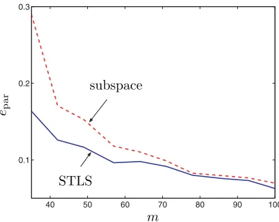
ex-periment; N = 100 repetitions of the experiment with different measurement noise realizations are performed. Figure 6.1 shows the average relative errors ¯epar for the
subspace method and for the STLS-based maximum likelihood method as a function of the time horizon m. The example shows that, for large sample sizes, the two ap-proaches give close estimates and, for small sample sizes, the subspace estimate can be improved by the STLS method.
40 50 60 70 80 90 100
0.1 0.2 0.3
m
¯
epar
subspace
[image:14.612.151.354.196.358.2]STLS
Fig. 6.1. Results for the system identification example: Average relative error of estimation
for the subspace and STLS methods.
6.2. MIMO system model reduction. Finite horizon 2-norm optimal model reduction can be formulated as an STLS problem with a block-Hankel structured data matrix. On the other hand, balanced model reduction [18], like subspace identifica-tion, does not require initial approximation but also does not minimize a particular cost function. Again an improvement can be expected over the balanced model reduc-tion method when the STLS method is used on a second stage of the approximareduc-tion. To illustrate the idea, consider the following example. A 10th order, 2-input, 1-output random system has to be approximated by an rth order system, where
r = 2,4,6,8. First we apply balanced reduction. The obtained solution is used as an initial approximation for the STLS method. Table 6.1 shows the average relative
H2-errors of approximation over N= 100 repetitions:
¯
eH2 = 1
N
N
k=1
H¯ −Hˆ(k)
H2
H¯H
2 .
The example confirms that the STLS method can be used to improve the result of the balanced model reduction method.
Table 6.1
Results for the model reduction example: Average relative error of estimatione¯H2for balanced
model reduction (BMR) and STLS.
Method r= 2 r= 4 r= 6 r= 8
7. Conclusions. We considered an STLS problem with the structure of the data matrix, specified blockwise. Each of the blocks can be block-Toeplitz/Hankel structured, unstructured, or exact. It was shown that such a formulation is flexible and covers as special cases many previously studied structured and unstructured matrix approximation problems.
The numerical solution method of [13] was extended to the block-Toeplitz/Hankel case. The approach is based on an equivalent unconstrained optimization problem: minXr(X)Γ−1(X)r(X). We proved that under assumption (2.6) about the struc-ture of the data matrix, the weight matrix Γ is block-Toeplitz and block-banded. These properties were used for cost function and first derivative evaluation with com-putational cost linear in the sample size.
The extension to block-Toeplitz/Hankel structured matrices is motivated by iden-tification and model reduction problems for MIMO dynamical systems. Useful further extensions are (i) to consider a weighted quadratic cost function ΔpVΔp, withV >0 diagonal, and (ii) regularized STLS problems, where the cost function is augmented with the regularization term vec(X)Qvec(X). These extensions are still computable inO(m) flops per iteration.
Appendix. Derivation of the first derivative of the cost function f0. Denote byDthe differential operator. It acts on a differentiable functionf0:U →R,
whereU is an open set inRn×dand gives as a result another function, the differential off0,D(f0) :U×Rn×d→R. The differentialD(f0) is linear in its second argument,
i.e.,
D(f0) := df0(X, H) = trace
f0(X)H ,
(A.1)
and has the property
f0(X+H) =f0(X) + df0(X, H) + o(HF)
for allX ∈U and for allH ∈Rn×d. (The notation o(H
F) has the usual meaning: g(H) = o(HF) if and only if limHF→0g(H)/HF= 0.) The function f0 :U →
Rn×l is the derivative of f
0. We compute it by deriving the differential D(f0) and
representing it in the form (A.1), from whichf0(X) is extracted.
The differential of the cost function f0(X) = r(X)Γ−1(X)r(X) is (using the
rule for differentiation of an inverse matrix)
df0(X, H) = 2rΓ−1
⎡ ⎢ ⎣
Ha1
.. .
Ham ⎤ ⎥
⎦−rΓ−1dΓ(X, H) Γ−1r.
The differential of the weight matrix
Γ =V˜r=Er˜r˜=E ⎡ ⎢ ⎣
X˜a1−˜b1
.. .
X˜am−˜bm ⎤ ⎥
⎦˜a1X−˜b1 · · · ˜amX−˜bm
,
where ˜A =:˜a1 · · · am
, ˜ai∈Rn, and ˜B=: ˜
b1 · · · bm
, ˜bi∈Rd, is
dΓ(X, H) =E ⎡ ⎢ ⎣
H˜a1
.. .
H˜am ⎤ ⎥
⎦˜r+E˜r˜a1H · · · ˜amH.
WithMij ∈Rd×d denoting the (i, j)th block of Γ−1,
1
2df0(X, H) = m
i,j=1
ri MijHaj− m
i,j,k,l=1
rlMliHEa˜ic˜jXextMjlrl
= trace
m
i,j=1
ajri Mij− m
i,j,k,l=1
I 0Vc,ij˜ XextMjlrlrl Mli
H
,
so that
1 2f
0(X) =
m
i,j=1
ajri Mij− m
i,j=1
I 0Vc,ij˜ XextNji,
whereNji(X) := m
l=1Mjlrl· m
l=1rlMli.
Acknowledgments. We would like to thank A. Kukush, M. Schuermans, P. Lem-merling, N. Mastronardi, and D. Sima for helpful discussion on the STLS problem.
REFERENCES
[1] T. Abatzoglou, J. Mendel, and G. Harada,The constrained total least squares technique
and its application to harmonic superresolution, IEEE Trans. Signal Process., 39 (1991),
pp. 1070–1087.
[2] P. Benner, V. Mehrmann, V. Sima, S. Van Huffel, and A. Varga,SLICOT—a subroutine
library in systems and control theory, in Applied and Computational Control, Signal and
Circuits, Vol. 1, B. N. Datta, ed., Birkh¨auser, Boston, 1999, Chap. 10, pp. 499–539.
[3] G. Cirrincione, G. Ganesan, K. Hari, and S. Van Huffel,Direct and neural techniques
for the data least squares problem, in Proceedings of the International Symposium on the
Mathematical Theory of Networks and Systems (MTNS), Perpignan, France, 2000.
[4] B. De Moor,Structured total least squares andL2 approximation problems, Linear Algebra
Appl., 188–189 (1993), pp. 163–207.
[5] B. De Moor,Total least squares for affinely structured matrices and the noisy realization
problem, IEEE Trans. Signal Process., 42 (1994), pp. 3104–3113.
[6] B. De Moor and B. Roorda,L2-optimal linear system identification structured total least
squares for SISO systems, in Proceedings of the 33th Conference on Decision and Control
(CDC), Lake Buena Vista, FL, IEEE Control Systems Society, 1994, pp. 2874–2879.
[7] W. A. Fuller,Measurement Error Models, John Wiley, New York, 1987.
[8] G. H. Golub and C. F. Van Loan,An analysis of the total least squares problem, SIAM J.
Numer. Anal., 17 (1980), pp. 883–893.
[9] P. Guillaume and R. Pintelon,A Gauss–Newton-like optimization algorithm for “weighted”
nonlinear least-squares problems, IEEE Trans. Signal Process., 44 (1996), pp. 2222–2228.
[10] A. Kukush, I. Markovsky, and S. Van Huffel, Consistency of the structured total least
squares estimator in a multivariate errors-in-variables model, J. Statist. Plann. Inference,
to appear.
[11] P. Lemmerling, N. Mastronardi, and S. V. Huffel,Fast algorithm for solving the
Han-kel/Toeplitz structured total least squares problem, Numer. Algorithms, 23 (2000), pp. 371–
392.
[12] M. J. Levin,Estimation of a system pulse transfer function in the presence of noise, IEEE
Trans. Automat. Control, 9 (1964), pp. 229–235.
[13] I. Markovsky, S. Van Huffel, and A. Kukush,On the computation of the multivariate
structured total least squares estimator, Numer. Linear Algebra Appl., 11 (2004), pp. 591–
608.
[14] I. Markovsky, S. Van Huffel, and R. Pintelon,Block-Toeplitz/Hankel Structured Total
Least Squares, Tech. Rep. 03–135, Department of Electrical Engineering, K.U. Leuven,
Belgium, 2003.
[15] I. Markovsky, S. Van Huffel, and R. Pintelon,Software for Structured Total Least Squares
Estimation: User’s Guide, Tech. Rep. 03–136, Department of Electrical Engineering, K.U.
[16] I. Markovsky, J. C. Willems, S. Van Huffel, B. D. Moor, and R. Pintelon,Application
of Structured Total Least Squares for System Identification and Model Reduction, Tech.
Rep. 04–51, Department of Electrical Engineering, K.U. Leuven, Belgium, 2004.
[17] N. Mastronardi, P. Lemmerling, and S. Van Huffel,Fast structured total least squares
algorithm for solving the basic deconvolution problem, SIAM J. Matrix Anal. Appl., 22
(2000), pp. 533–553.
[18] B. C. Moore,Principal component analysis in linear systems: Controllability, observability
and model reduction, IEEE Trans. Automat. Control, 26 (1981), pp. 17–31.
[19] R. Pintelon and J. Schoukens,System Identification: A Frequency Domain Approach, IEEE
Press, Piscataway, NJ, 2001.
[20] J. B. Rosen, H. Park, and J. Glick,Total least norm formulation and solution for structured
problems, SIAM J. Matrix Anal. Appl., 17 (1996), pp. 110–126.
[21] M. Schuermans, P. Lemmerling, and S. Van Huffel,Structured weighted low rank
approx-imation, Numer. Linear Algebra Appl., 11 (2004), pp. 609–618.
[22] S. Van Huffel, ed., Recent Advances in Total Least Squares Techniques and
Errors-in-Variables Modeling, SIAM, Philadelphia, 1997.
[23] S. Van Huffel and P. Lemmerling, eds.,Total Least Squares and Errors-in-Variables
Mod-eling: Analysis, Algorithms and Applications, Kluwer Academic, Dordrecht, The
Nether-lands, 2002.
[24] S. Van Huffel and J. Vandewalle,Analysis and properties of the generalized total least
squares problemAX≈Bwhen some or all columns in Aare subject to error, SIAM J.
Matrix Anal. Appl., 10 (1989), pp. 294–315.
[25] S. Van Huffel and J. Vandewalle,The Total Least Squares Problem: Computational Aspects
and Analysis, SIAM, Philadelphia, 1991.
[26] P. Van Overschee and B. De Moor,Subspace Identification for Linear Systems: Theory,