The use of Kriging in stochastic model updating and its effect on parameter estimates

THE USE OF KRIGING IN STOCHASTIC MODEL UPDATING

AND ITS EFFECT ON PARAMETER ESTIMATES

Liang, P., DiazDelaO, F.A., Patelli, E., and Mottershead, J.E.

Institute of Risk and Uncertainty, School of Engineering, University of Liverpool, Liverpool L69 3GH, UK.

E-mail of the corresponding author: [email protected]

SUMMARY: The Kriging predictor or Gaussian process emulator is a commonly used surrogate model for reduc-ing the computational cost in the forward propagation of model updatreduc-ing. It has already been used and discussed by many other researchers. As a stochastic model, the Kriging predictor provides not only the mean value of the prediction but also the prediction variance. Previous work mainly used the prediction variance as a kind of judge-ment on the model accuracy during the selection of design points and took only the mean value of the predictor in the further study and production of results. Therefore, the model updating result obtained from only the mean value of the Kriging predictor may be considered not accurate enough because of neglecting the prediction vari-ance information. In order to investigate the effect of the Kriging prediction varivari-ance on parameter estimates, an approach is developed in this paper for including it in model updating procedure. The approach is based on a trans-fer method for the prediction variance and bootstrap algorithm. The main steps and the assumptions are presented, followed by numerical examples using a univariate model updating problem. The results obtained show the effect of the Kriging prediction variance on parameter estimates and are compared to results produced by conventional methods that neglect the Kriging prediction variance in model updating.

KEYWORDS:Model updating, Kriging, prediction variance.

1. INTRODUCTION

The Kriging model is a very commonly used interpolation technique. It provides an efficient surrogate model for the expensive forward propagation in model updating. Previous work on model updating with the Kriging model mainly considered the mean value of the Kriging prediction. However, the prediction variance of the Kriging model also affects the model-updating result. It indicates the accuracy of the Kriging prediction and therefore also affects the parameters estimated by the model updating process using the Kriging model. The Kriging prediction variance was used for selecting new design points to obtain a better Kriging model [1][2][3], for global optimisation of time-consuming Monte-Carlo simulation [4], and for measuring the quality of the prediction of a Kriging model [5]. In this paper, the Kriging prediction variance will be used with a variance transfer method and the bootstrap technique in order to estimate the its effect on the parameters estimated by model updating with Kriging.

The rest of this article is organised as follows. The univariate problem concerned will be presented in Section 2. Section 3 introduces the background theory of model updating using the Kriging model and kernel density estima-tion. Section 4 explains the procedure for including the Kriging prediction variance in the model updating result. The numerical examples are given in Section 5 for the univariate model-updating problem. A brief introduction of the Kriging model, and the description of the model updating method with Kriging are provided in the Appendix.

2. THE UNIVARIATE PROBLEM

Figure 1 shows a 3-dof mass-spring system. It consists of three masses and six springs. The stiffnessk2is selected

as the updating parameter in this case study, and the third eigenvalue of the systemω₃2is selected as the response

to be used for updatingk2. Hence, for the Kriging model used as surrogate,k2is the input andω₃2is the output.

Other parameters in the system are determined as following.

k1=k3=0,k4=1.9N/m or k4=2.0N/m,k5=2.0N/m,k6=1.0N/m

The feasible range of parameterk2is chosen as [6.5,9.5].

Figure 1 – 3-dof mass-spring system

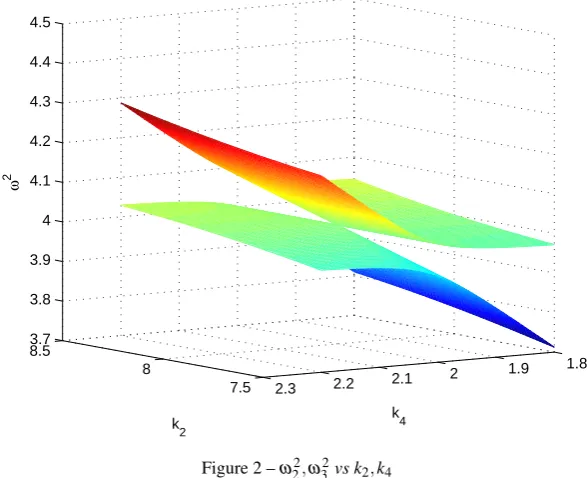
Figure 2 presents the surfacesω₂2andω₃2with differentk2,k4values. The two surface are quite close to each other and connect at the point(k2,k4) = (8,2)N/m, so that the response of the highest eigenvalue is represented by a

curveω₃2(k2)with a slope discontinuity whenk4=2N/m. The discontinuity then occurs atk2=8N/m. This

particular case is that of crossing eigenvalues and is chosen especially because it presents a challenging problem

for the Kriging model and for the model updating. Any other value ofk4results in veering of the eigenvalues. We

selectk4=1.9N/mandk4=2.0N/mas two cases for our particular study. The case ofk4=1.9N/mis a more

usual problem with a smooth response curveω₃2(k2). The method described in the following two sections will be

applied to these two problems and the results will be compared.

7.5 8

8.5

1.8 1.9 2

2.1 2.2 2.3 3.7

3.8 3.9 4 4.1 4.2 4.3 4.4 4.5

k

4

k

2

ω

2

Figure 2 –ω₂2,ω₃2vs k2,k4

3. BACKGROUND THEORY

A brief introduction of the background theory, including iterative model updating with a Kriging model, the prin-ciple of the kernel density estimation, and the bootstrap algorithm for density estimations, to be used in the model updating process will be presented in this section.

3.1. Model Updating with Kriging Predictor

This method is described by Haddad Khodaparast et al [5] who gave recursive equation for the updating parameter as (Eq. 25, [5])

θ

θθl+1= (HTH+D+U+V−A+W)−_θθθ=1θθθl{f(θθθ) +H

T

µµµ−HTΛρΛρΛρ−g(θθθ) +Wθθθ}_θθθ=θθθl (1)

This equation comes from the optimisation problem minθ(εTε), whereεis the error vector between measurement

z_m and Kriging predictor outputˆz. The explanation of the matrices in Equation 1 is provided in the Appendix.

More details of the derivation of the recursive equation equation (1) can be found in [5].

3.2. Kernel Density Estimation

Kernel density estimation fX(x,σ) = 1

σn√2π∑ n

j=1exp ₋

(x−x(j))2

2σ2

will be implemented for estimating the

proba-bility distribution of the updated parameters from a limited number of samples. As this kernel density estimator

uses the normal distribution kernel, the smoothing parameter of the estimator, or the bandwidthhis equivalent to

the standard deviationσ in the kernel density function. In the specific case of normal distributed target function,

the bandwidth is given byσ=

4 ˆσ5

3n

1₅

, where ˆσis the standard deviation of the samples andnis the sample size.

This estimation is optimal for estimating normal underlying densities. It should be noted that theσ in the kernel

density estimation function is different from the ˆσ in the bandwidth function.σ is the standard deviation of the

kernel, and ˆσis the standard deviation of the samples to be estimated.

3.3. Bootstrap Algorithm for Density Estimation

The bootstrap is a re-sampling method for assigning measures of accuracy to sample estimates. It is the practice of estimating properties of an estimator by measuring those properties when sampling from an approximating dis-tribution. Bootstrap algorithm can be utilised for estimating the variation of density estimates [6]. New estimates are constructed with re-sampled data and the variation of the estimates is obtained by by the repeated bootstrap re-sampling to determine re-constructed density estimates. The algorithm is described in the following steps:

If{xi;i=1, ...,n}is a set of data with probability densityp. The bootstrap algorithm for this data is as follows [6]: 1. Form density estimate ˆpfrom data{xi;i=1, ...,n}.

2. Resample (uniformly)n values from{xi;i=1, ...,n}, with replacement, obtaining{x∗i;i=1, ...,n}

(boot-strap data). Note that in resampling with replacement our boot(boot-strap dataset may contain the sameximultiple

times.

3. Form density estimate ˆp∗from data{x∗_i;i=1, ...,n}.

4. Repeat steps 2&3Ntimes to obtain a family of bootstrap density estimates{pˆ∗_i;i=1, ...,N}. 5. The distribution of ˆp∗_i about ˆpmimics the distribution of ˆpaboutp.

The bootstrap density estimates reproduce the variance of ˆp, and it is a useful tool for estimating the variance of a density estimator.

4. ESTIMATING OF THE PROBABILITY DISTRIBUTION OF THE UPDATED PARAMETERS

In this section, an approximate calculation method for determining the covariance matrix of the random variables is presented. The Jacobian matrix between the output and input of the Kriging model is derived and will be used for the covariance calculation by linearisation of the input-output relationship from the Kriging predictor. The Kriging prediction covariances will then be included in the model updating by re-sampling from the derived parameter covariances. Kernel density estimates are constructed with the re-sampled data and its confidence intervals are evaluated with the bootstrap algorithm.

4.1. Linear approximation using predicting variance from the Kriging model

In order to include the variance information given by the Kriging model in estimating parameters, a linear approxi-mation will be used to transfer the Kriging output variance to parameter variance. We assume the parameter/output relationship to be linear in the local area around an updated parameter. The parameter covariance matrix can be determined from the outut prediction covariance matrix given by the Kriging model. A general form of a

transfor-mation between input vectorθθθand output vectorZcan be expressed as

whereJis the Jacobian matrix betweenXandY. MatrixJcan be presented as J=        ∂z1 ∂ θ1

∂z1 ∂ θ2 · · ·

∂z1 ∂ θp ∂z2

∂ θ1 ∂z2 ∂ θ2 · · ·

∂z2 ∂ θp ..

. ... ...

∂zn ∂ θ1

∂zn ∂ θ2 · · ·

∂zn ∂ θp

       (3)

Then, the relationship betweenCovZ, the covariance matrix ofZ, andCovθθθ, the covariance matrix ofθθθ, can be written as

CovZ=JCovθθθJT (4)

By using this equation, we can transfer the variance betweenθθθandZ.

Specifically, for the Kriging model used in this report, the Jacobian matrix for the model in Equation 15 can be written as

J=JI+JII (5)

whereJIis the Jacobian matrix of the regression part,β0,i+bTiθθθ+12θθθTBiθθθ, of the Kriging model.

JI= 

   

b1T+θθθTB1 b2T+θθθTB2

.. .

bnT+θθθTBn



   

|θθθ=θθθ∗

(6)

JIIis the Jacobian matrix for the other part,λλλT_iri(θθθ).

JII=       

∂ λλλT₁r1(θθθ) ∂ θθθ ∂ λλλT₂r2(θθθ)

∂ θθθ .. . ∂ λλλTnrn(θθθ)

∂ θθθ

      

|θθθ=θθθ∗

(7)

where

∂ λλλT_i ri(θθθ)

∂ θθθ = h

∂ λλλT_iri(θθθ)

∂ θ1

∂ λλλT_iri(θθθ)

∂ θ2 · · ·

∂ λλλT_iri(θθθ)

∂ θp

i

(8)

∂ λλλT_iri(θθθ) ∂ θt

=−ζt,iνi·λ_iT      

(−1)s_|θ

t−θt(1)|νi−1Ci(θθθ,θθθ(1)) (−1)s|θt−θt(2)|νi−1Ci(θθθ,θθθ(2))

.. .

(−1)s_|θ

t−θt(ns)|νi−1Ci(θθθ,θθθ(ns)₎

     

, s=

(

0 θt≥θt(h)

1 θt<θ

(h)

t

(9)

The equations above based on the differentiability of the Kriging model, which is related to the chosen of the correlation function.

For a single updated valuedof the parameter from the Kriging model updating, with the calculated parameter

vari-anceσk, a new sample should be sampled from the distributionN(d,σk). A kernel density estimate is constructed

with the new samples of all the updated parameter values, and the confidence intervals of this density estimate is evaluated by bootstrapping. The whole process can be summarised as:

1. Deterministic model updating with the constructed Kriging model using equation (1). 2. Evaluate the variance of the updated parameters using equation (4).

3. Re-sample using a different dataset taken from the distribution of the updating parameters. 4. Evaluate the kernel density estimate of each of the new samples.

5. NUMERICAL EXAMPLES

In this section, the numerical implementation of the model updating methodology will be presented using several numerical simulation case studies. The simulation will be carried out for the univariate problem of the mass-spring system. The procedure will be introduced in the following order.

• Multiple deterministic model updating and the updated parameter distribution determined using kernel

den-sity estimation. In this section, the uncertainty caused by the Gaussian process of the Kriging predictor will not be taken account.

• Determining the distribution of the input, or updating parameter (stiffness) from the known distribution

on the output (natural frequency) by the approximate calculation using linearisation of the input-output relationship from the Kriging predictor. The uncertainty from the Kriging predictor will be taken account in the determination.

• Approximate calculation of output distribution by Monte Carlo simulation. The result of the simulation

taking account and not taking account of the uncertainty from the Kriging model will both be presented.

For constructing the Kriging model, design points need to be sampled from the feasible range ofk2. As this is

a univariate problem, the sampling of the Kriging predictor started with three points,k2=6.5,8.0,9.5, two end

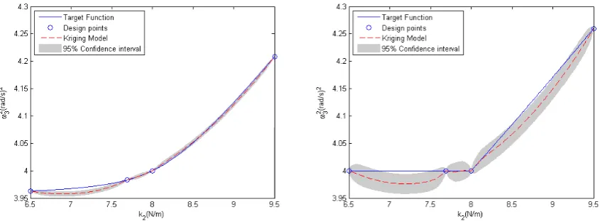
points and the middle point in the feasible range. A sequential procedure was used for design point sampling with new design points added using the the maximal MSE criterion [2][7]. A quite coarse Kriging situation with only 4 design points was deliberately constructed for the two casesk4=1.9N/mandk4=2.0N/m. Figure 3 shows

the target functions given by mathematical models and the Kriging predictors. The second function is with slope

discontinuity atk2=8N/mcannot be modelled accurately by Kriging with only 4 design points marked by circles

in Figure 3 and the 95% confidence interval of the Kriging predictors shown as a shaded region. It is obvious that the Kriging model is less good in the case of the second target function. Surrogate models are needed as substitutes for expensive FE-models. The purpose of constructing a Kriging predictor here is to demonstrate a strategy for combining the Kriging predictor as a part of the a model updating procedure that fully takes account of the Kriging variance.

Figure 3 – The 4 point Kriging model of the univariate system. Left:k4=1.9N/m. Right:k4=2.0N/m.

The model updating process is based on the Kriging predictor. Two sets of synthetic observation samples are used for the comparison of the model updating results. The first sample sets consists of 10 samples, and the other one consists of 100 samples. The sample generating method is as follows.

1. Generating parameterk2from distributionN(8.5,0.5).

2. Calculating the correspondingω₃2(k2)using the mathematical model.

3. Mixing the calculatedω₃2values with noise generated fromN(0,0.001).

By using this procedure, the uncertainty in the measurement comes from two parts, the parameter uncertainty and measurement noise.

5.1. Estimation of Parameter Distribution using Deterministic Model Updating

Model updating was applied for each measurement sample, and the initial value ofk2for updating was set as

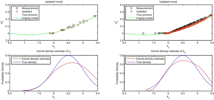
Updated results of two measurement sets for two cases are shown in Figure 4 and 5. Kernel density estimates for updated parameters were compared with the true parameter densities (N(8.5,0.5)). The kernel density estimates differ from the true densities because of an insufficient number of Kriging training points and from each other because of the different numbers of samples used. But as the true parameter density would be unknown for a real application, this density estimation is the maximum information that can obtained based on the current method. Additionally, as the second function concerned in this case study contains a horizontal line where the eigenvalue is insensitive to the parameter, the model updating results in this region cannot be expected to be accurate. This problem also influences the accuracy of the parameter kernel density estimate. The parameter updating of strictly non-monotonic functions would be a topic to be studied in the future.

6.5 7 7.5 8 8.5 9 9.5

3.95 4 4.05 4.1 4.15 4.2 4.25 k 2 ω3 2 Updated result Measurement Updated True process Kriging model

6.5 7 7.5 8 8.5 9 9.5

0 0.2 0.4 0.6 0.8 1 k 2 Probability Density

Kernel density estimate of k

2

Kernel density estimate True density

6.5 7 7.5 8 8.5 9 9.5

3.95 4 4.05 4.1 4.15 4.2 4.25 k 2 ω3 2 Updated result Measurement Updated True process Kriging model

6.5 7 7.5 8 8.5 9 9.5

0 0.2 0.4 0.6 0.8 k 2 Probability Density

Kernel density estimate of k

2

Kernel density estimate True density

Figure 4 – Model updating results of 4 point Kriging model,k4=1.9N/m. Left: 10 samples. Right: 100 samples.

6.5 7 7.5 8 8.5 9 9.5

3.9 4 4.1 4.2 4.3 4.4 k 2 ω3 2 Updated result Measurement Updated True process Kriging model

6.5 7 7.5 8 8.5 9 9.5

0 0.2 0.4 0.6 0.8 k 2 Probability Density

Kernel density estimate of k

2

Kernel density estimate True density

6.5 7 7.5 8 8.5 9 9.5

3.9 4 4.1 4.2 4.3 4.4 k 2 ω3 2 Updated result Measurement Updated True process Kriging model

6.5 7 7.5 8 8.5 9 9.5

0 0.2 0.4 0.6 0.8 k 2 Probability Density

Kernel density estimate of k

2

Kernel density estimate True density

Figure 5 – Model updating results of 4 point Kriging model,k4=2.0N/m. Left: 10 samples. Right: 100 samples.

5.2. Inclusion of Kriging Variance Information

updating parameter. However, the Kriging model only holds for perfect fitting at its design points. At other points, the response calculated by the Kriging model is usually slightly different from the true model. As a result of this small difference, the updated parameter values found with the Kriging model will slightly biased from the correct value. The model updating based on the mean value of the Kriging model gives only one possible result in the confidence interval of the Kriging model. There will be other valid points within the density of the Kriging outputs that should be considered.

5.3. Updating using Kriging Variance Data and Bootstrapping

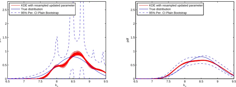
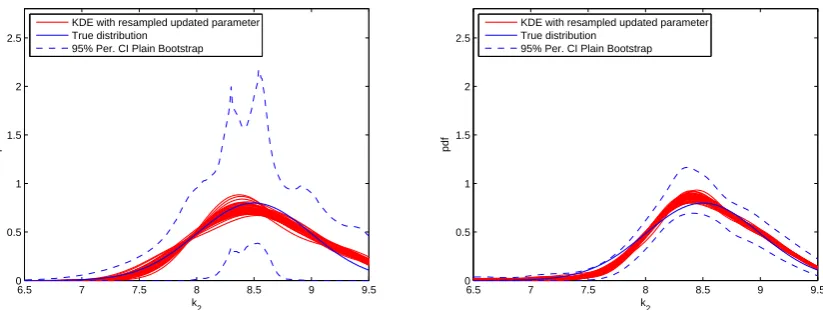
Figures 6 and 7 show the comparison of results from two different sample sizes for the two cases concerned. The true distribution is denoted by the blue curve. The red curves are kernel density estimates obtained by sampling from parameter densities obtained by inversion of equation (4). The blue dashed lines are 95% confidence intervals obtained by bootstrapping. It can be seen that the confidence intervals in all cases enclose the red curves. Also the general shape of the red curves and boundaries of the confidence intervals are similar. As the sample size increases, the variation of the re-constructed density estimates reduces and the confidence intervals become narrower. The crossing-modes curve with the greater Kriging prediction variance also creates greater variance in the parameter densities. The results for thek4=2.0N/mcase with a 12 design point model is shown in Figure 8. As the Kriging

prediction variance gets smaller with more design points, the variation of the result also becomes smaller compared to the 4 design-point case.

6.5 7 7.5 8 8.5 9 9.5

0 0.5 1 1.5 2 2.5

k

2

pdf

KDE with resampled updated parameter True distribution

95% Per. CI Plain Bootstrap

6.5 7 7.5 8 8.5 9 9.5

0 0.5 1 1.5 2 2.5

k

2

pdf

KDE with resampled updated parameter True distribution

95% Per. CI Plain Bootstrap

Figure 6 – Bootstrapping results of the 4 point Kriging model,k4=1.9N/m. Left: 10 samples. Right: 100 samples.

6.5 7 7.5 8 8.5 9 9.5

0 0.5 1 1.5 2 2.5

k

2

pdf

KDE with resampled updated parameter True distribution

95% Per. CI Plain Bootstrap

6.5 7 7.5 8 8.5 9 9.5

0 0.5 1 1.5 2 2.5

k

2

pdf

KDE with resampled updated parameter True distribution

95% Per. CI Plain Bootstrap

6.5 7 7.5 8 8.5 9 9.5 0

0.5 1 1.5 2 2.5

k

2

pdf

KDE with resampled updated parameter True distribution

95% Per. CI Plain Bootstrap

6.5 7 7.5 8 8.5 9 9.5

0 0.5 1 1.5 2 2.5

k

2

pdf

KDE with resampled updated parameter True distribution

95% Per. CI Plain Bootstrap

Figure 8 – Bootstrapping results of the 12 point Kriging model,k4=2.0N/m. Left: 10 samples. Right: 100 samples.

6. CONCLUSION

This paper addresses the use of Kriging model in model updating and presents a method to incorporate the effect of Kriging prediction variance in the estimation of model-updating parameters. Numerical implementations for a univariate problem are described and the results obtained show the effect of Kriging prediction variance on the model updating result. It shows that the Kriging prediction variance does produce an evident influence on model updating results based on a Kriging model. Therefore for obtaining a more precise result, the prediction variance of Kriging model should be considered in the model updating procedure and the method provided in the article could be used to estimate the effect of Kriging prediction variance.

APPENDIX

Kriging predictor

A Universal Kriging predictor can be presented as

Z(θθθ) =

k

∑

j=1

βjfj(θθθ) +ε(θθθ) (10)

The random functionZ(θθθ)includes a regression model∑kj=1βjfj(θθθ), and a random processε(θθθ).ε(θθθ)is assumed to have mean zero and covarianceCov(θθθ,ϑϑϑ) =σ2C(θθθ,ϑϑϑ) between ε(θθθ) andε(ϑϑϑ), where σ2 is the process variance andC(θθθ,ϑϑϑ)is the correlation.

In this report, a second order polynomial is used for the regression part in the Kriging model. Hence, the Kriging model of thei-th output is expressed as

ˆ

zi=β0,i+bTiθθθ+ 1 2θθθ

T_B

iθθθ+εi(θθθ) (11)

whereθθθ= [θ1,θ2,· · ·,θp]T is the uncertain system parameter vector.bTi = [β1,i,β2,i,· · ·,βp,i]T,

Bi=



   

2β11,i β12,i · · · β1p,i 2β22,i · · · β2p,i . ._. .._.

sym. 2βpp,i



   

, and the covariance ofεi(θθθ)is

cov(εi(θθθ),εi(ϑϑϑ)) =σi2Ci(θθθ,ϑϑϑ) (12)

Ci(θθθ,ϑϑϑ) =

p

∏

j=1

Cj,i(θj,ϑj) (13)

The mean Kriging predictor may be expressed as

ˆ

zi=β0,i+bTiθθθ+ 1 2θθθ

T_B

iθθθ+λλλTiri(θθθ) (15)

whereri(θθθ) = [Ci(θθθ,θθθ(1)),Ci(θθθ,θθθ(2)),· · ·,Ci(θθθ,θθθ(ns)_)]T_,θθθ(1)_{,· · ·,θθθ}(ns)_{are the design points, andλλλ}

i=R−i 1(Z:,i−

Ξ ΞΞ[[[β])

The training of the Kriging predictor starts with a few initial training points. Ghoreyshi et al [2] used Latin hyper-cube sampling (LHS) to generate initial points and a central composite design (CCD) was used in [5]. In this study, a one dimensional system is used and the initial points are chosen as three points which are the two boundaries points and the middle point of the region. Sacks et al [1] introduced several design criteria including Integrated Mean Squared Error (IMSE), Maximum Mean Squared Error (MMSE), and Entropy. The MMSE criterion will be used in this study. The maximum point of mean squared error (MSE) of Kriging predictor will be used to determine the location of the new point in iteration.

For a Kriging predictor expressed as equation (10). The MSE for this predictor can be expressed as

MSE(zˆi(θθθ)) =σi2[1− fT(θθθ) rT(θθθ)

0 FT

F R

−1

f(θθθ) r(θθθ)

(16)

where ˆzi(θθθ)is the linear predictor ofzi(θθθ)at an untriedθθθ.f(θθθ) = [f1(θθθ),· · ·,fk(θθθ)]Tis the vector ofkfunctions in

the regression,F=



 

fT(θθθ(1))

.. .

fT(θθθ(ns)) 



is thens×kexpanded design matrix,R=R(θθθ (i)_,

θ

θθ(j)),1≤i≤ns; 1≤j≤nsis the

ns×nsmatrix of stochastic-process correlations between the design points, andr(θθθ) = [R(θθθ(1),θθθ),· · ·,R(θθθ(ns),θθθ)]T is the vector of correlations between design points and an untriedθθθ.

The goal of the MMSE criterion is to minimise

max θθθ∈ΘΘΘ

MSE[(zˆi(θθθ)] (17)

In each training step, the MSE of the predictor is calculated and a maximum MSE point will be added to training points in the next training step. Thus, the MSE of predictor will be reduced step by step with the increasing of the number of training points. The training iteration stopped when the maximum MSE falls under a chosen threshold.

Model updating recursive equation

In the model updating recursive equation

θ

θθl+1= (HTH+D+U+V−A+W)−_θθθ=1θθθl{f(θθθ) +H

T

µµµ−HTΛρΛρΛρ−g(θθθ) +Wθθθ}_{θθθ=θθθ}

l

the process matricesH,D,U,V,A,f,g,W,µµµ,,,ΛΛΛare

H(θθθ) = [Hi j]n×p; Hi j=βj,i+θjβj j,i+ 1 2

p

∑

k=1,k6=j

βk j,iθk

n– the number of the Kriging outputs, p– the number of Kriging inputs,ns – the number of the Kriging design

points

D(θθθ) = [Di j]p×p; Di j= 1 2

p

∑

k=1

n

∑

l=1

Hl j

∂Hl j

∂ θi

+Hlk

∂Hl j

∂ θi

θk

U(θθθ) = [Ui j]p×p; Ui j= n

∑

k=1

ns

∑

l=1 λl,kHk j

∂rl,k(θ)

∂ θi

V(θθθ) = [Vi j]p×p; Vi j= n

∑

k=1

ns

∑

l=1 λl,k

∂Hk j

∂ θi

rl,k(θ)

A= [Ai j]p×p; Ai j= n

∑

k=1 µk

∂Hi j

∂ θi

; ∂Hi j

∂ θi

=1

2Bi j,k

f(θθθ) ={fi(θ)}p×1; fi(θ) = n

∑

j=1

ns

∑

k=1 λk,jµj

∂rk,j(θ)

g(θθθ) ={gi(θ)}p×1; gi(θ) = 1 2

n

∑

l=1

ns

∑

k=1

ns

∑

j=1 λj,lλk,l

r_k,l(θ)

∂rj,l(θ)

∂ θi

+r_j,l(θ)

∂rk,l(θ)

∂ θi

µµµ=zm−βββ0

ΛΛΛ= 

  

λ1,1 λ2,1 · · · λns,1 0 · · · 0 0 · · · 0 λ1,2 · · · λns,2 0 · · · 0

· · · · · · λns,n



  

λ λ

λi= (λi,1,λi,2,· · ·,λi,n)T =R−i1(Zi−Fβββ)

MatrixWis chosen to make(WTW+D+U+V−A+W)invertible. It may be chosen in the formW=λI.Bi j,k

is the component of matrixBkwhich is a parameter matrix in the Kriging predictor expression equation (11).

REFERENCES

[1] Sacks, J., Welch, W., Mitchell, T., Wynn, H., “Design and Analysis of Computer Experiments”, Statistical Science, 4(4), 1989, pp. 409–423.

[2] Ghoreyshi, M., Badcock, K.J., Woodgate, M.A., “Accelerating the Numerical Generation of Aerodynamic Models for Flight Simulation”, Journal of Aircraft, 46(3), 2009, pp. 972–980.

[3] Kleijnen, J.P.C., Beers, W.C.M.v., “Application-Driven Sequential Designs for Simulation Experiments: Krig-ing MetamodellKrig-ing”, The Journal of the Operational Research Society, 55(8), 2004, pp. 876–883.

[4] Jones, D., “A Taxonomy of Global Optimization Methods Based on Response Surfaces”, Journal of Global Optimization, 21(4), 2001, pp. 345–383.

[5] Khodaparast, H.H., Mottershead, J.E., Badcock, K.J., “Interval model updating with irreducible uncertainty using the Kriging predictor”, Mechanical Systems and Signal Processing, 25(4), 2011, pp. 1204–1206.

[6] Narsky, I., Porter, F.C., Density Estimation, Wiley-VCH Verlag GmbH & Co. KGaA, 2013, pp. 89–120.

[7] Kleijnen, J.P.C., “Kriging metamodeling in simulation: A review”, European Journal of Operational Research, 192(3), 2009, pp. 707–716.