This is a repository copy of Dual Response Choices in Pivoted Stated Choice Experiments.
White Rose Research Online URL for this paper: http://eprints.whiterose.ac.uk/43618/
Article:
Rose, JM and Hess, S (2009) Dual Response Choices in Pivoted Stated Choice Experiments. Transportation Research Record, 2135. 25 - 33 . ISSN 0361-1981
https://doi.org/10.3141/2135-04
Reuse See Attached
Takedown
If you consider content in White Rose Research Online to be in breach of UK law, please notify us by
DUAL RESPO SE CHOICES I PIVOTED STATED CHOICE EXPERIME TS
John M. Rose* and Stephane Hess John M. Rose
The University of Sydney
Faculty of Economics and Business
Institute of Transport and Logistics Studies Newtown, NSW 2006, Australia
Tel: +61 (0)2 9351 0168 Fax: +61 (0)2 9351 0088
Stephane Hess
Institute for Transport Studies, University of Leeds
& Institute of Transport and Logistics Studies, University of Sydney Tel: +44 (0)113 34 36611
Fax: +44 (0)113 343 5334
* corresponding author
Word count:
Text 5646
Tables 2 x 250 = 500 Figures 3 x 250 = 250
ABSTRACT
I TRODUCTIO
The question as to whether or not to include a ‘status quo’ alternative (sometimes referred to as a ‘no choice’ or ‘opt out’ alternative in various literatures) in stated choice (SC) studies has been widely debated in many discipline areas, but appears to have been largely ignored within the transportation literature. In the nonAtransport related literature, significant differences in results of SC experiments with and without the presence of status quo alternatives have been found (see e.g., (1)), and in general, the recommendation has been that status quo alternatives should be used in such experiments (e.g., (2) – (4)). These recommendations have grown from a number of arguments that have been put forward for the use of status quo alternatives. These arguments include that the inclusion of a status quo alternative leads to an increase in the realism of SC tasks (see e.g., (5) – (7)), an increase in the external validity of welfare estimates derived from SC experiments (see e.g., (2)) and an improvement in the statistical efficiency of parameters estimated from discrete choice models (see e.g., (8) – (9)). For a further overview of these arguments, see e.g., (10) – (11)).
Traditionally, where used, the no choice or status quo alternative has been represented in SC data as either being an alternative labelled as ‘none’ and devoid of any attribute levels or alternatively as an option labelled as ‘your current alternative’ with attribute levels given simply as “at the current level” (see e.g., (1), (10), (12)). Whilst both versions of the status quo alternative have different implications given different interpretational meanings (i.e., the ‘none’ option represents a complete optAout of all nonAstatus quo alternatives by the respondent whereas the “your current alternative” option represents the choice of an already experienced or known alternative and hence is not strictly a no choice alternative), it is the impact upon respondents of including such alternatives in SC experiments that requires careful consideration. Where a ‘none’ option is used, there exists little possibility of interpretation differences in terms of what the alternative means to respondents as the choice of selecting none of the other alternatives presented within a choice task should have the same meaning for the entire sample. Where the status quo alternative is described simply as “your current alternative” however, interpretation differences may arise as different respondents may have different current alternatives, or in the case where all respondents face the same status quo alternative, may possess different perceptions as to the current attribute levels that that alternative possesses. As such, it is likely that SC experiments using “at the current level” status quo alternatives will likely exhibit heterogeneity in the error terms for the status quo alternative whereas it is not certain that questionnaires using ‘none’ type status quo options will naturally induce such heterogeneity.
respondents are asked what their perceptions are of the attribute levels for a current (usually chosen) real world alternative, and these are used as an alternative in the choice tasks that they view1. In this way, the perceptions of these levels are revealed to the analyst rather than remaining unknown. Thus, whilst reference alternatives may also induce preference heterogeneity similar to “at the current level” status quo alternatives, this preference heterogeneity need not be unexplainable.
Brazell et al. (14) outline several problems that may arise from the use of a status quo alternative in SC experiments, problems that may also exist with the use of reference alternatives. They argue that when selected, no information is captured on the relative attractiveness of the other non status quo alternatives. This suggests that the parameter estimates associated with the non status quo alternatives are obtained from fewer observations as the number of times the status quo alternative is selected over the sample increases. Further, if the pattern of choosing the status quo alternative is such that there is a concentration of such choices on certain choice tasks in the experiment, then the experiment may loose statistical power, not only due to a lack of data, but also via impacts on the information matrix which may result in certain biases in the econometric modelling.
In addition to detailing possible issues related to the use of status quo alternatives, Brazell et al. (14) also provide a single solution that potentially solves all the issues they identified simultaneously. This solution involves the use of dual responses in SC experiments where respondents are first asked to select from amongst all non status quo alternatives (a forced choice) after which they are asked to make a second choice in which the status quo alternative is added (a nonAforced choice). The use of dual responses in SC experiments, whilst potentially improving the statistical efficiency of estimated models as well as providing further information that can be used to refine the parameter estimates, may however lead to other potential modelling problems, in particular violations of the identical and independently distribute (IID) assumption if the data from the two choices are pooled into a single data set. IID violations may occur if the error variances between the two choice tasks are different. Brazell et al. (14) acknowledge this potential problem, and found that in simulated data as well as in two empirical data sets, no such violations occur. Nevertheless, Dhar and Simpson (11) who also explore issues related to the use of dual responses within SC choice tasks, did find limited evidence of such violations occurring.
In this paper, we seek to explore similar issues to those raised by Brazell et al. (14). However, in doing so, we use a modified version of the dual response format typically used elsewhere. In the current study, we use two empirical data sets in which respondents are first asked to select from three alternatives; a respondent specific reference alternative and two hypothetical SC alternatives, after which they are asked to select from the two hypothetical alternatives only if they selected the reference alternative in the first instance. In capturing response data in this manner, the demands placed on respondents
1
completing the survey are somewhat limited, provided that they do not always select the reference alternative in making their first set of choices. As such, this method seeks to minimise respondent burden, whilst still capturing information on the preferences of the nonAreference alternatives. In addition to examining whether there exist violations of IID between the two response tasks, we also seek to examine whether there exist differences in the marginal willingness to pay (WTP) in the form of values of travel time savings (VTTS) of respondents between the observed choices. Such differences were seemingly largely ignored by other researchers, with the assumption being that only error variances differ between the two choice tasks.
The remainder of the paper is organised as follows. The next section looks at survey design and sampling. We then turn our attention to model specification before presenting the results of our empirical applications. Finally, we present the conclusions of the research.
SURVEY DESIG A D SAMPLI G
The SC Experiment
Two separate SC experiments were used to collect data to examine route choice behaviour; one involving commuters and the other nonAcommuters. Both experiments invited respondents to review three alternatives consisting of a reference alternative and two hypothetical SC alternatives. In total, respondents were asked to review 16 choice tasks each. Based on the attribute levels of the alternatives, respondents were initially asked to select their preferred alternative from the three presented to them. If respondents chose the reference alternative out of these three options, then they were given a secondary choice between the two hypothetical alternatives. The survey instrument employed was a computer aided personal interview (CAPI).
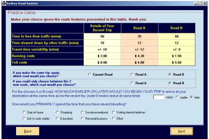
The alternatives in each survey task were each described by five attributes; free flow and slowed down times, trip time variability, and two cost attributes, running (petrol) and toll costs. For each respondent, the attributes of the first alternative were always described using the attribute levels of a recent trip that respondents were asked about earlier in the
survey. The attribute levels of the two hypothetical SC alternatives were constructed as percentages around the first reference alternative. To demonstrate how the experimental
desing approach works, consider two respondents, the first of whom indicated that they spent 15 minutes in free flow traffic conditions whilst the second claims to have spent 30 minutes. Assume that in constructing the experiment, the analyst used as pivot levels A
25, 0 and 25 percent. Over the course of the experiment, the freeAflow attribute of the reference alternative would remain at 15 minutes for the first respondent and 30 minutes
for the second. The attribute levels that would be shown to the first respondent for the hypothetical alternatives however would consist of 11.25, 15 and 18.75 minutes whilst
the second respondent would see 22.5, 30 and 37.5 minutes as levels for the freeAflow attribute. In employing this form of experimental design approach, the levels shown to each respondent are thus tailored to the respondents own experiences. An example choice
the example shown, the respondent claimed to have spent 50 minutes in free flow conditions and 10 minutes in congested traffic conditions for their most recent trip. The
25 and 40 minute free flow times shown for hypothetical roads A and B represent a 50 percent and 20 percent reduction in time spend in free flow time respectively from the current reference alternative time, whilst the 12 minutes shown for the slowed down time
represents a 20 percent increase in the current reference alternative time of 10 minutes. The allocation of the times shown is given by the underlying experimental design.<
Figure 1 Here >
The Underlying Experimental Design
For the present study, separate efficient designs were generated for the two segments examined as part of the study. Given a set of attributes and attribute levels, efficient designs are constructed such that the levels are allocated to the design in such a way that the elements (or subsets thereof) of the varianceAcovariance (VC) matrix are expected to be minimised once data is collected. Rather than work with the elements in the VC matrix directly, the literature suggests working with different measures that summarise the values that populate the VC matrix. One such measure is the DpAerror, which is given as
(
1)
1( ) k,
I β − (1)
which is the determinant of the inverse of the Fisher Information matrix, I, for a design given a particular econometric model form and certain parameter estimates, ,β scaled by one over the number of parameters, k. That is, the VC matrix of the model is calculated for the set of parameter estimates obtained for that model.
In order to calculate Equation (1) for a design, the analyst must first assume a set of prior parameter estimates. If these are not known with certainty (as would typically be expected), the analyst may use prior parameter estimates drawn from Bayesian distributions and calculate the Bayesian DAerror statistic, DbAerror, which is represented as
(
1)
1(
1)
1det ( ) k det ( ) k.
k
Eβ I β − = I β −
∫
(2)To generate a DAefficient design, whether Bayesian parameter priors are assumed or not, different attribute level allocations are tested, with attribute level combinations that produce lower DAerror values representing more statistically efficient designs. Such designs are expected to produce data that will maximise the tAratios for the design parameters (for further discussion on the generation of such designs, see e.g., (16)A(26)).
Greene (13). The precise method used to construct the experimental designs, given the presence of reference alternatives, is discussed in Rose et al. (26).
The Sample
The data used in this paper were collected in Sydney, Australia, in 2004. Two segments of data were collected as part of the study; commuter and nonAcommuter car drivers. Respondents from both segments were asked to make a series of choices from a range of alternatives defined in terms of travel times and costs. Individuals included in the sample were only those who had recently undertaken an eligible trip, defined as a trip where the respondent could have reasonably used an existing toll road in the Sydney catchment area over the previous seven days. To ensure that a large number of travel circumstances were captured, quotas were imposed on various travel times (called trip length segmentation). To ensure some variety in trip length, three segments were investigated: no more than 30 minutes, 31 to 60 minutes, and more than 61 minutes (capped at two hours). A geographically stratified sampling plan was also employed to ensure a spread of originA destinations in the trips sampled. Telephone calls were used to make initial contact and survey recruitment. Upon agreeing to participate in the survey, a time and location was agreed upon for a faceAtoAface CAPI. The final data consists of 467 effective interviews of which 243 represent commuter trips and 224 nonAcommuter trips.
Figure 2 shows how the survey sampling and questions were implemented in practice. Firstly, respondents were recruited into different trip type and trip length categories. Once recruited into a particular category, respondents were then asked to complete the survey instrument which consisted of three parts; initial questions related to a recent trip they made; 16 SC questions similar to that shown in Figure 1; and finally attitudinal and socioAdemographic questions. As shown in Figure 2, different efficient designs were generated for each of the quota segments.
< Figure 2 Here >
Data used for modelling purposes: First and second preference choice data
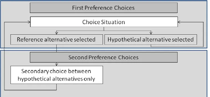
For each of the 16 choice tasks, respondents were asked to make either one or two choices. In each task, respondents were first asked to select from either their reference alternative or one of two hypothetical SC alternatives. Only if the reference alternative was selected as their preferred option were respondents then asked to make a second choice from amongst the two hypothetical SC alternatives. Figure 3 shows within choice set process used in the survey, highlighting the differences between the first and secondary choices that respondents were asked to make.
< Figure 3 Here >
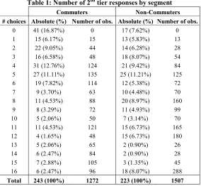
alternative as their first preference in all 16 choice tasks (which represents a form of nonA trading behaviour; see e.g., (27)), compared to 16.87 and 7.62 percent of commuters and nonAcommuters respectively not selecting the reference alternative in any of the 16 choice tasks.
< Table 1 here >
Five models are estimated on each data set (i.e., commuter and nonAcommuter data sets), thus producing a total of 10 models. The five models (by two segments) are estimated using subsets of the choice observations from the full set of data such that each model is estimated using
M1: First preference choices only
M2: Second preference choices only, including second preferences for choice situations where reference alternative was not chosen
M3: Only second preference choice observations excluding observations where a SC alternative was selected as the first preference
M4: Pooled first and second choice observation data (excluding observations where a SC alternative was selected as the first preference)
M5: Pooled first and second choice observation data (excluding observations where a SC alternative was selected as the first preference) accounting for scale differences
As well as including second preference choice observations, model M2 also includes choice observations where a nonAreference alternative was selected in the first preference task. Thus, model M2 also includes those second preference choice observations in which the respondent was not forced to declare a different alternative as their next best preference (i.e., the respondent did not choose the reference alternative as their first preference). In some way, this would however mean that choices for these observations would be overweighted. For models M3 to M5, only choice observations where a respondent was forced to select a second preference alternative were included in the analysis (i.e., the respondent choose the reference alternative as their first preference). As such, the number of choice observations per respondent for the second choice task will range between zero and 16 depending on how many times they selected the reference alternative as their first preference). Model M1 used only the first preference task ignoring any second preferences that have been declared.
MODEL SPECIFICATIO
All estimated models use the same general form of the utility specification. The utility functions for the models are given as Equations (3a) to (3b).
( ) ref ref ref
U ref =δ +βx +ε (3a)
1 1 1
1
( ) sp sp sp
U sp =δ +βx +ε (3b)
2 2
2
( ) sp sp ,
where x represents the freeAflow time, slowed down time, travel time variability, vehicle running costs and toll cost attributes and the β the associated parameter estimates.
In estimating each of the models, the attribute related parameter estimates are specified as being generic across the reference and hypothetical SC alternatives. Alternative specific constants are estimated for the reference and first SC alternatives to capture inertia effects as well as left to right biases in respondents answering the SC questions.
Models M1, and M2 and M3 look separately at the first and second choices and as such are not affected by possible scale differences. For models M4 and M5, which pool the first and second preference data subsets, the parameters are constrained to be generic across the pooled data sets. For model M5, a scale parameter was estimated for the second preference choice data to account for possible differences in the error variances between the two choice tasks.
MODEL RESULTS
The focus of the present analysis was on testing for differences between first and second responses rather than on intricate exploration of advanced methodological issues such as interArespondent taste heterogeneity. Furthermore, no correlation between the errors for the different alternatives could be retrieved. With this in mind, we limited ourselves to Multinomial Logit (MNL) models. However, two departures from standard methodology were incorporated in that model M5 allows for scale differences between first and second responses and in that all models were estimated using Jackknife approaches to account for the pseudo panel nature of the data and correct the standard errors (see e.g., (28)). The results are given in Tables 2 and 3 for the commuter and nonAcommuter data segments respectively.
< Table 2 here >
< Table 3 here >
time variability parameter is found to be statistically significant only in model M2 (commuter and nonAcommuter).
Model M5 is estimated on the same pooled data as model M4, however an additional scale parameter is estimated allowing for different error variances for the two choice sets. The scale parameter for both the commuter and nonAcommuter segments are not statistically significant at the 95 percent level compared to the important value of one (not zero) suggesting that the error variances for the first and second preferences are not statistically different, although the scale parameter is statistically significant for the commuter data at the 93 percent level. This lack of differences in the error variances is reflected in the fact that the model results are almost identical for Models M4 and 5. The fact that there is no statistical evidence that the error variances are different suggests that no violation of the IID assumption occurs in either data set from the pooling the two choices into a single data set, thus supporting the earlier finding of Brazell et al. (14).
Tables 2 and 3 also report the VTTS for the 10 models. Given that there exist two cost parameters, VTTS estimates for the freeAflow and slowed down time attributes are reported against each. All VTTS are given in AU$ per minute. Asymptotic tAratios for each VTTS are given in each table and 95 percent confidence intervals are reported separately at the bottom of each of the tables. All VTTS values are statistically different from zero except for the freeAflow time against running cost estimate in model M3 for the commuter data segment. As is to be expected, the average VTTS are higher for the commuter segment than for the nonAcommuter segment, with the exceptions of Model M1 (slowed down time versus running cost) and M3 (slowed down time versus toll cost).
Examination of the 95 percent confidence intervals for the VTTS suggests that within each data segment there exist overlapping estimates for the VTTS. Within each model, comparing the VTTS reported, in only a few cases do the confidence intervals not overlap. Indeed, only in models M4 and M5 estimated on the commuter sample do the VTTS for slowed down time estimated against running cost not overlap with all the other VTTS estimated within that particular model (e.g., in models M4 and 5, the slowed down time estimated against running cost confidence interval ranges from $0.26 to $0.34 whereas the range for the freeAflow time against toll cost VTTS is between $0.13 and $0.23).
other models, including those for model M3 nonAcommuter. Despite the VTTS obtained from M3 nonAcommuter not being statistically different to the VTTS generated from other models, the values themselves do on face value appear to be more different than those obtained from any other pairwise VTTS comparison.
DISCUSSIO A D CO CLUSIO
This study examines the issue of dual response data, specifically for SC experiments involving respondent defined reference alternatives. Unlike traditional dual response data which typically use as the status quo alternative a ‘no choice’ or at ‘your current level’ alternative, the data used herein uses as the base alternative a respondent defined reference alternative. These individual specific alternatives differ from the traditional type of base alternatives in that each respondent provides the levels for the alternative from which the hypothetical alternatives are generated. Whilst the use of reference alternatives in this manner is not new, we examine (for what we believe to be the first time) the option of capturing more than one response per choice observation for such data. Further, unlike some other research on dual response data, we have employed a strategy that captures data on respondents’ second preferences only if they indicate that they prefer the reference or status quo alternative in the first instance. In this way, it is believed that the cognitive burden to which respondents are exposed is minimised.
Similar to Brazell et al. (14) but in contrast to Dhar and Simpson (11), we find no systematic violations of the IID assumption caused by the pooling of the first and second preference data across two separate empirical data sets, although it should be noted that for one data set, the commuter data set, the scale parameter was almost statistically different at the 95 percent confidence level. One possibility for the similarity between our findings and those of Brazell et al. (14), and the contradictory results with those of Dhar and Simpson (2003) may lie in the complexity of the choice experiments examined in these studies. In Dhar and Simpson (11), a simple experiment involving only two attributes per alternative was used, whereas the experiments reported in Brazell et al. (14) and here are more complex, involving many more attributes. The existence of larger number of attributes may assist in distinguishing between the alternatives, as well as remove the possibility that no clear compromise alternative exists within a given choice task. Whilst further research is warranted on this issue, if this is the cause, then care should be given to overly simple experimental designs when using dual response type data. In making the above statement, we note however that much research has already been conducted on the influences that different design dimensions, such as the number alternatives, attributes, attribute levels, and attribute level ranges, play on the on SC behavioural outcomes (see e.g., (29)A(34). Caussade et al. (29) and Chintakayala et al. (30) in particular examine the influence each dimension plays on the error variances of respondents, and found that different aspects of experimental designs do influence the error variances of those answering SC questions.
dual response type data. Our findings suggest that no systematic differences exist between the VTTS for dual response type data, although some differences were found for the VTTS derived from the worst performing model estimated. Given that the other models appear to perform much better than this model however, both in terms of model fit and statistically significant behavioural outputs, we are inclined to discount the results from this finding and conclude that on the balance of probabilities, that the VTTS do not differ across the dual response data, whether estimated as pooled or separate data sources.
REFERE CES
(1) Dhar, R. (1997) Consumer Preference for a NoAChoice Option, Journal of Consumer Research, 24, 215A231.
(2) Adamowicz, W. and P. Boxall (2001) Future Directions of Stated Choice Methods for Environment Valuation, paper prepared for: Choice Experiments: A /ew Approach to Environmental Valuation, April, London, England.
(3) Bennett, J. and Blamey, R. (2001) The Choice Modelling Approach to Environmental Valuation, Edward Elgar.
(4) Bateman, I., Carson, R.T., Day, B., Hanemann, M., Hanley, N., Hett, T., JonesALee, M., Loomes, G., Mourato, S.,Ozdemiroglu, E., Pearce, D.W., Sugden, R., and Swanson, J. (2003) Economic Valuation with Stated Preference Techniques: A Manual (in association with the DTLR and DEFRA), Edward Elgar.
(5) Louviere, J.J. and Woodworth, G. (1983) Design and analysis of simulated consumer choice or allocation experiments: an approach based on aggregate data. Journal of Marketing Research, 20, 350A367.
(6) Batsell, R. and Louviere, J.J. (1991) Experimental Analysis of Choice, Marketing Letters, 2(3), 199A214.
(7) Carson, R., Louviere, J.J., Anderson, D., Arabie, P., Bunch, D., Hensher, D.A, Johnson, R., Kuhfeld, W., Steinberg, D., Swait, J., Timmermans, H., and Wiley, J. (1994) Experimental Analysis of Choice. Marketing Letters, 5 (October), pp351A367.
(8) Louviere, J.J. and Hensher, D.A. and Swait, J.D. (2000) Stated Choice Methods: Analysis and Application, Cambridge University Press, Cambridge.
(9) Anderson, D.A. and J.B. Wiley (1192) Efficient Choice Set Designs for Estimating Available CrossAEffects Models, Marketing Letters, 3(4), 357A370.
(10) Kontoleon, A. and Yabe M. (2003) Assessing the Impacts of Alternative ‘Opt Out’ Formats in Choice Experiment Studies: Consumer Preferences for Genetically Modified Content and Production Information in Food, Journal of Agriculture Policy and Research, 5, 1A43.
(11) Dhar, R. and Simonson, I. (2003) The effect of forced choice on choice, Journal of Marketing Research, 40(2), 146A160.
(12) Tversky, A. and E. Shafir (1992) Choice Under Conflict: The Dynamics of Deferred Decision, Psychological Science, 6, 358A361.
(13) Hensher, D.A. and Greene, W.H. (2003) The Mixed Logit model: The state of practice.
Transportation, 30 (2) 133A176.
(14) Brazell, J.D., Diener, C.G., Karniouchina, E., Moore, W.L., Severin, V. and Uldry, P.F. (2006) The noAchoice option and dual response choice designs, Marketing Letters, 17, 255A268.
(15) Train, K. and Wilson, W. (2008) Estimation on statedApreference experiments constructed from revealed preference choice, Transportation Research Part B, 42(3), 191A203.
(17) Toner, J.P., Clark, S.D., GrantAMuller, S.M. and Fowkes, A.S. (1999) Anything you can do, we can do better: a provocative introduction to a new approach to stated preference design, WCTR, Antwerp, 3, 107A120.
(18) Sándor, Z., and Wedel, M. (2001) Designing Conjoint Choice Experiments Using Managers’ Prior Beliefs, Journal of Marketing Research, 38, 430A444.
(19) Sándor, Z., and Wedel, M. (2002) Profile Construction in Experimental Choice Designs for Mixed Logit Models, Marketing Science, 21, 455A475.
(20) Sándor, Z., and Wedel, M. (2005) Heterogeneous conjoint choice designs, Journal of Marketing Research, 42, 210A218.
(21) Bliemer, M.C.J., and Rose, J.M. (2006) Designing Stated Choice Experiments: StateA ofAtheAart, paper presented at the 11th International Conference on Travel Behaviour Research, Kyoto, Japan.
(22) Kanninen, B.J. (2002) Optimal Design for Multinomial Choice Experiments, Journal of Marketing Research,39, 214A217.
(23) Kessels, R., Goos, P. and Vandebroek, M. (2006) A comparison of criteria to design efficient choice experiments, Journal of Marketing Research, 43, 409A419.
(24) Rose, J.M. and Bliemer, M.C.J. (2006) Designing efficient data for stated choice experiments. Paper presented at the 11th International Conference on Travel Behaviour Research, Kyoto, Japan.
(25) Ferrini, S. and Scarpa, R.S (2007) Designs with aApriori information for nonAmarket valuation with choice experiments: A Monte Carlo study, Journal of Environmental Economics and Management, 53, 342A363.
(26) Rose, J.M., Bliemer, M.C.J., Hensher, D.A. and Collins, A.C. (2008) Designing Efficient Stated Choice Experiments Involving Respondent Based Reference Alternatives, Transportation Research Part B, 42(4), 395A406.
(27) Hess, S., Rose, J.M. and Polak, J.W. (2008), Nontrading, Lexicographic, and Inconsistent Behaviour in StatedAPreference Choice, paper presented at the 87th Annual Meeting of the Transportation Research Board, Washington, D.C.
(28) Cirillo, C., Daily, A. and Lindveld, K. (2000) Eliminating Bias Due to the Repeated Measurements Problem in SP Data, in Ortuzar, J. de D. (Ed.) Stated Preference Modeling Techniques, London: PTRC.
(29) Caussade, S., Ortúzar, Juan de Dios Ortúzar, J., Rizzi L. and Hensher, D.A. (2005) Assessing the Influence of Design Dimensions on Stated Choice Experiment Estimates, Transportation Research Part B, 39 (7), 621-640.
(30) Chintakayala, P.K., Hess, S. Rose, J.M. and Wardman, M. (2009) Effects of stated choice design dimensions on estimates, International Choice Modelling Conference, March 30-April 1, Yorkshire U.K.
(31) Hensher, D.A. (2004) Accounting for Stated Choice Design Dimensionality in Willingness to Pay for Travel Time Savings, Journal of Transport Economics and Policy, 38 (2), 425-446.
(33) Hensher, D.A. (2006b) Revealing differences in behavioural response due to the dimensionality of stated choice designs: an initial assessment, Environmental and Resource Economics, 34 (1), May, 7-44.
LIST OF TABLES A D FIGURES
Table 1: umber of 2nd tier responses by segment Table 2: Commuter model results
Table 3: on1Commuter model results
Figure 1: An example of a stated choice screen Figure 2: Survey instrument phases
Table 1: umber of 2nd tier responses by segment
Commuters on1Commuters
# choices Absolute (%) umber of obs. Absolute (%) umber of obs.
0 41 (16.87%) 0 17 (7.62%) 0
1 15 (6.17%) 15 13 (5.83%) 13
2 22 (9.05%) 44 14 (6.28%) 28
3 16 (6.58%) 48 18 (8.07%) 54
4 31 (12.76%) 124 21 (9.42%) 84
5 27 (11.11%) 135 25 (11.21%) 125
6 19 (7.82%) 114 12 (5.38%) 72
7 9 (3.70%) 63 10 (4.48%) 70
8 11 (4.53%) 88 20 (8.97%) 160
9 8 (3.29%) 72 11 (4.93%) 99
10 5 (2.06%) 50 7 (3.14%) 70
11 11 (4.53%) 121 15 (6.73%) 165
12 4 (1.65%) 48 15 (6.73%) 180
13 5 (2.06%) 65 2 (0.90%) 26
14 6 (2.47%) 84 2 (0.90%) 28
15 7 (2.88%) 105 3 (1.35%) 45
16 6 (2.47%) 96 18 (8.07%) 288
[image:18.595.157.441.108.370.2]Table 2: Commuter model results
M1a M2a M3a M4a M5a
Par. (tAratio) Par. (tAratio) Par. (tAratio) Par. (tAratio) Par. (tAratio) Ref. Constant 0.274 (1.75) 0.204 (2.98) 0.351 (4.55) 0.327 (2.13) 0.327 (2.10)
SP1 Constant 0.077 (1.22) A A A A 0.207 (3.77) 0.201 (3.58)
Free Flow Time A0.069 (A7.31) A0.065 (A9.19) A0.055 (A4.94) A0.066 (A8.65) A0.068 (A8.62) Slowed Down time A0.091 (A20.20) A0.083 (A23.96) A0.049 (A4.13) A0.085 (A23.20) A0.087 (A20.39)
Running Cost A0.314 (A14.25) A0.279 (A11.00) A0.192 (A4.06) A0.285 (A11.40) A0.293 (A12.11) Toll Cost A0.361 (A17.46) A0.364 (A14.85) A0.384 (A12.05) A0.369 (A18.54) A0.376 (A18.37) Travel Time Variability A0.006 (A0.84) A0.029 (A2.96) A0.032 (A1.30) A0.007 (A0.99) A0.007 (A0.96)
Alpha A A A A A A A A 0.848 (A1.85)*
Parameter differences
Par. Diff. (tAratio) Par. Diff. (tAratio) Par. Diff. (tAratio) Par. Diff. (tAratio) Par. Diff. (tAratio) Free FlowA Slowed Down Time 0.022 (4.51) 0.018 (3.20) A0.007 (A0.55) 0.019 (4.14) 0.019 (4.18)
Running A Toll Cost 0.047 (1.95) 0.085 (3.61) 0.192 (4.93) 0.084 (4.06) 0.083 (3.9)
Model Fits
LL(0) A4271.405 A2694.956 A881.683 A5153.088 A5153.088
LL(β) A3027.662 A1814.977 A693.266 A3751.375 A3748.716
Adjusted ρ2 0.29 0.324 0.207 0.271 0.271
Number of Observations 3888 3888 1272 5160 5160
WTP (Au$ /per minute)
WTP (tAratio) WTP (tAratio) WTP (tAratio) WTP (tAratio) WTP (tAratio) Free Flow Time A Running Cost $0.22 (6.80) $0.23 (8.31) $0.29 (3.91) $0.23 (7.65) $0.23 (7.79) Slowed Down Time A Running Cost $0.29 (10.57) $0.30 (13.73) $0.25 (8.90) $0.30 (13.80) $0.30 (13.53)
Free Flow Time A Toll Cost $0.19 (8.47) $0.18 (6.58) $0.14 (1.76) $0.18 (7.10) $0.18 (7.44) Slowed Down Time A Toll Cost $0.25 (14.99) $0.23 (15.04) $0.13 (4.10) $0.23 (16.32) $0.23 (16.16)
M1 M2 M3 M4 M5
Lower 95 % Upper 95 % Lower 95 % Upper 95 % Lower 95 % Upper 95 % Lower 95 % Upper 95 % Lower 95 % Upper 95 %
Free Flow Time A Running Cost $0.16 $0.28 $0.18 $0.29 $0.14 $0.43 $0.17 $0.29 $0.17 $0.29 Slowed Down Time A Running Cost $0.24 $0.34 $0.25 $0.34 $0.20 $0.31 $0.26 $0.34 $0.26 $0.34 Free Flow Time A Toll Cost $0.15 $0.23 $0.13 $0.23 ;$0.02 $0.30 $0.13 $0.23 $0.13 $0.23 Slowed Down Time A Toll Cost $0.22 $0.28 $0.20 $0.26 $0.07 $0.19 $0.20 $0.26 $0.20 $0.26
Table 3: on1Commuter model results
M1b M2b M3b M4b M5b
Par. (tAratio) Par. (tAratio) Par. (tAratio) Par. (tAratio) Par. (tAratio) Ref. Constant 0.226 (1.69) 0.356 (6.30) 0.576 (10.73) 0.347 (2.68) 0.347 (2.63)
SP1 Constant 0.136 (2.08) A A A A 0.347 (6.91) 0.348 (6.90)
Free Flow Time A0.069 (A7.11) A0.066 (A9.11) A0.054 (A5.20) A0.065 (A8.73) A0.066 (A8.81) Slowed Down time A0.085 (A10.72) A0.081 (A9.47) A0.066 (A5.79) A0.081 (A11.28) A0.082 (A10.21)
Running Cost A0.314 (A6.66) A0.316 (A8.83) A0.286 (A7.35) A0.312 (A8.87) A0.315 (A7.81) Toll Cost A0.411 (A13.72) A0.033 (A13.70) A0.039 (A8.93) A0.411 (A14.65) A0.414 (A14.02) Travel Time Variability 0.009 (1.58) 0.009 (A3.00) 0.009 (A1.90) 0.007 (1.44) 0.008 (1.41)
Alpha A A A A A A A A 0.959 (A0.47)*
Parameter differences
Par. Diff. (tAratio) Par. Diff. (tAratio) Par. Diff. (tAratio) Par. Diff. (tAratio) Par. Diff. (tAratio) Free FlowA Slowed Down Time 0.017 (2.88) 0.015 (2.14) 0.012 (0.99) 0.017 (3.17) 0.017 (3.15)
Running A Toll Cost 0.097 (3.64) A0.283 (3.37) A0.247 (3.01) 0.099 (4.63) 0.099 (4.59)
Model Fits
LL(0) A3919.849 A2473.149 A1044.573 A4964.421 A4964.421
LL(β) A2731.63 A1616.098 A768.656 A3526.202 A3525.981
Adjusted ρ2 0.301 0.344 0.258 0.288 0.288
Number of Observations 3568 3568 1507 5075 5075
WTP (Au$ /per minute)
WTP (tAratio) WTP (tAratio) WTP (tAratio) WTP (tAratio) WTP (tAratio) Free Flow Time A Running Cost $0.22 (5.12) $0.21 (7.77) $0.19 (4.91) $0.21 (6.79) $0.21 (6.41) Slowed Down Time A Running Cost $0.27 (10.93) $0.26 (13.55) $0.23 (8.55) $0.26 (13.78) $0.26 (14.22)
Free Flow Time A Toll Cost $0.17 (4.53) $0.17 (4.55) $0.14 (2.90) $0.16 (4.43) $0.16 (4.04) Slowed Down Time A Toll Cost $0.21 (9.15) $0.20 (8.84) $0.17 (5.48) $0.20 (9.72) $0.20 (9.26)
M1 M2 M3 M4 M5
Lower 95 % Upper 95 % Lower 95 % Upper 95 % Lower 95 % Upper 95 % Lower 95 % Upper 95 % Lower 95 % Upper 95 %
Free Flow Time A Running Cost $0.13 $0.30 $0.16 $0.26 $0.11 $0.26 $0.15 $0.27 $0.14 $0.27 Slowed Down Time A Running Cost $0.22 $0.32 $0.22 $0.29 $0.18 $0.28 $0.22 $0.30 $0.22 $0.30 Free Flow Time A Toll Cost $0.08 $0.26 $0.09 $0.24 $0.04 $0.23 $0.09 $0.23 $0.08 $0.23 Slowed Down Time A Toll Cost $0.16 $0.25 $0.16 $0.25 $0.11 $0.22 $0.16 $0.24 $0.16 $0.24
[image:20.595.110.772.88.500.2]