promoting access to White Rose research papers
Universities of Leeds, Sheffield and York
http://eprints.whiterose.ac.uk/
This is an author produced version of a paper accepted for publication in
Computational Materials Science.
White Rose Research Online URL for this paper:
http://eprints.whiterose.ac.uk/42990/
Paper:
Ye, JQ, Lam, D and Zhang, DX (2010) Initiation and propagation of transverse
cracking in composite laminates. Computational Materials Science, 47 (4). 1031 – 1039.
ACCEPTED FOR PUBLICATION IN COMPUTATIONAL MATERIALS SCIENCE
Initiation and Propagation of Transverse Cracking in Composite Laminates
Jianqiao Ye1*, Dennis Lam1 and Daxu Zhang2
1
Institute for Resilient Infrastructure (iRI), School of Civil Engineering, University of Leeds, Leeds, LS2 9JT, UK
2
School of Mechanical, Aerospace and Civil Engineering, University of Manchester, PO Box 88, Manchester, M60 1QD, UK.
Abstract
The matrix cracking transverse to loading direction is usually the one of most
common observations of damages in composite laminates. The initiation and
propagation of transverse cracks have been a longstanding issue in the last few
decades. In this paper, a three-dimensional stress analysis method based on the state
space approach is used to compute the stresses, including the inter-laminar stresses
near transverse cracks in laminated composites. The stress field is then used to
estimate the energy release rate, from which the initiation and propagation of
transverse cracking are predicted. The proposed method is illustrated by numerical
solutions and is validated by available experimental results. To the best knowledge of
the authors, the predictions of crack behaviour for non-symmetrical laminates and
laminates subject to in-plane shearing are presented for the first time in the literature.
Introduction
The first form of damages in laminates is usually matrix microcracks. The most
common observation of microcracking is cracking in 90º plies during axial loading in
the 0º directions (Narin, 2000). Transverse cracking is therefore the most common
damage mode in composite materials. An immediate effect of transverse cracking is to
cause stiffness degradations of the laminate. Stress singularities near the crack tips at
the ply interface may initiate interlaminar delamination. Delamination is not
necessarily the ultimate structural failure, but it may result in fibre-matrix debonding
ultimate failure of a composite laminate follows the occurrence of transverse cracking,
longitudinal cracking, delamination and fibre breaking.
The initiation and propagation of transverse cracks in composite laminates
have been the focus of failure investigation in the last few decades. Extensive
investigations have been carried out both experimentally and analytically.
Garrett and Bailey (1977), Parvizi et al. (1978) and Bailey and Parvizi (1981)
are amongst the earliest researchers who carried out extensive experiments to observe
transverse cracks. They found that cracks formed in a direction parallel to the
transverse reinforcement and the thickness of the 90° plies had significant effect on
the cracking process. Flaggs and Kural (1982) presented the results of an
experimental study confirming that the constrained transverse cracking phenomena
observed in the 90° ply of uniaxially loaded [0°/90°]s composite laminates was also
exhibited by the more general [θ/90°]s class of composite laminates. Nairn and Hu
(1992), Liu and Nairn (1992) and Nairn et al. (1993) carried out a series of
experiments on crack density as a function of applied load. For all the laminates
tested, the characteristic cracking curve had no cracks until an onset stress was
reached. After the initial crack, the crack density typically increases very rapidly. The
onset stress decreases as the thickness of the 90° plies increases. Yokozeki et al.
(2005) investigated crack accumulation in multiple plies of [0/θ2/90°]s laminates
(θ=30°, 45° and 60°). Most of the experimental investigations showed that the first
damage mode was usually transverse cracking. Both the thickness of 90° layers and
the stiffness of constrain layers affected the initiation and propagation of transverse
cracks.
The majority of earlier analytical work on transverse cracking assumed that
cracks formed when the stress or strain reached the transverse strength of a ply
material. Garrett and Bailey (1977) assumed that a transverse ply had a unique
breaking strain, εtu, and strength σtu. If a stress is applied in a direction parallel to the
longitudinal plies, the transverse ply will fail at a stress σtu. Using the same strength
criteria, Parvizi, et al (1978) reported more detailed studies for a glass fibre reinforced
epoxy composite. Leblond et al. (1996) studied multiplication of transverse cracks as
a function of applied stress in cross-ply laminates. The crack development was
assumed to be controlled by the fracture stress in the 90° plies. However the strength
the strength of 90o plies of a laminate is usually not the same as that of a different
laminate.
Due to the drawbacks and limitations of the strength based methods, the
majority of recent work was based fracture mechanics using the energy method to
predict transverse cracking. Most energy models used a representative volume
element (RVE) to predict next crack formation when the energy released due to crack
formation reached the critical strain energy release rate Gc. It has been widely
recognised that for the same material ply laminates with different lamination profiles,
the value of Gc almost keeps constant (Nairn, 2000). Consequently, the method
applies for a wide variety of laminates from a single value of Gc.
Parvizi et al. (1978) demonstrated that a simple shear lag analysis used in
conjunction with the Griffith energy criterion can be used to accurately predict matrix
cracking. Flaggs (1985) made use of a strain energy release rate fracture criteria in
conjunction with an approximate two-dimensional shear-lag model to predict tensile
matrix failure. Wang et al (1985) employed the energy release rate method of classical
fracture mechanics to model various matrix crack interactions. Dvorak and Laws
(1987) investigated the first ply failure using a critical energy release rate criteria and
later Laws and Dvorak (1988) presented a model for progressive transverse cracking
based on statistical fracture mechanics. Nairn (1989; 2000), Liu and Nairn, (1992) and
Nairn and Hu (1992) carried out a series of study on matrix cracking by finite fracture
mechanics. Zhang et al. (1992) and Fan and Zhang (1993) proposed the equivalent
constraint model (ECM), in which the energy release rate due to transverse ply
cracking, incorporating residual thermal stresses, was derived. McCartney (1998;
2002; 2004; 2005) investigated ply crack development for various lamination profiles;
from cross-ply to general symmetric laminates, subjected to axial extension or mixed
mode loading. Smith and Ogin (1999) calculated the critical bending moment at
transverse cracking under flexural loads using a fracture mechanics approach. Joffe et
al. (2001) used a crack-closure technique to calculate the energy release caused by
cracking. A Monte-Carlo simulation in incremental strain-controlled loading was used
to model the transverse cracking process. The 90° layer was divided into a large
number of elements and a critical energy release rate Gc was assigned to each element
release rates associated with crack propagation in the width direction were calculated
using a three-dimensional FEA. Subsequently Yokozeki et al. (2005) used the same
method to study micro-cracking behaviour induced by matrix cracks in adjacent plies.
Lim and Li (2005) calculated energy release rates for transverse cracking and
delamination under the generalised plane strain condition. By introducing the
minimum strain energy density criterion to a non-linear FE analysis, Sirivedin et al.
(2006) predicted matrix crack propagation in continuous-carbon fibre/epoxy
composites.
It is obvious that for an energy based method, an accurate prediction of the
stress distribution within a RVE is essential to an accurate estimate of the potential
energy within the element. This is particularly difficult for a laminated RVE with
transverse cracks. Traditional analysis of laminated composites used classic or higher
order plate theories that usually provided unsatisfactory predictions to interfacial
stresses and the stress singularities at the tips of transverse cracks. Zhang and Ye
(2007a) recently developed an analytical model that can provide accurate predictions
to the stress fields, including all the interfacial stresses, and a satisfactory
approximation to the stress singularities near ply cracks. The model was based on a
state space approach that has been successfully used to solve a variety of stress
problems (Soldatos and Ye, 1994; Ye and Soldatos, 1994a, b, 1995; Ye and Sheng,
2003; Ye et al., 2004; Zhang and Ye, 2007b). Compared with other analytical models,
this new model takes full three-dimensional consideration of laminar properties,
displacements and interfacial stress continuities at all material interfaces. The model
can also deal with both symmetric and non-symmetric laminates with a universal
approach. A comprehensive account of the methodology can be found in Ye (2002).
In combination with the state space formulation (Ye, 2002) this paper presents
a model to predict crack propagation by using an energy based approach. An accurate
stress distribution within a RVE with cracks is obtained from the state space solution.
The stresses are then used to compute the energy release rate in the crack propagation
analysis. Numerical results are obtained and compared with the tests results available
in the literature. Results are also presented for non-symmetric laminates and laminates
subjected to in-plane shearing. From the authors’ best knowledge, these results are
Solution of an angle-ply lamina
Consider an off-axis lamina (Fig. 1) with principal material directions (1-2-3) in the
global x-y-z coordinate system. The lamina has constant thickness h, width L and
infinite length. The displacements in the x, y and z directions are denoted by u, v and w, respectively. Suppose that the lamina is subjected to a uniform tension by the
application of a constant longitudinal strain in the y direction, ε0 ,which represents a
laminate that is long and relatively uniform in one direction, such as aircraft wing
panels. The constant strain in the y direction also represents the state of stress at a
point in a material subject to a generalized plane strain, where the stresses and strains
in other two directions are more dominating.
The lamina is made of a homogeneous, monoclinic and linearly elastic material
whose principal material direction 1, i.e., the fiber direction, has an angle of θ to the x
axis.
(a) Stress-strain relations
The basic constitutive equation for thermo-elastic stress analysis is (Herakovich, 1998)
{ }
σ =[ ]
C({ }
ε −{ }
εT ). (1) Here, the matrices[ ]
C ,{ }
ε and{ }
εT are stiffness matrix, total strains and thermal strains, respectively. For a linearly elastic monoclinic material,[ ]
⎥ ⎥ ⎥ ⎥ ⎥ ⎥ ⎥ ⎥ ⎦ ⎤ ⎢ ⎢ ⎢ ⎢ ⎢ ⎢ ⎢ ⎢ ⎣ ⎡ ′ ′ ′ ′ ′ ′ ′ ′ ′ ′ ′ ′ ′ ′ ′ ′ ′ ′ ′ ′ = 66 36 26 16 55 45 45 44 36 33 23 13 26 23 22 12 16 13 12 11 0 0 0 0 0 0 0 0 0 0 0 0 0 0 0 0 C C C C C C C C C C C C C C C C C C C CC , (2)
where the Cij′ are stiffness coefficients that can be expressed in terms of Young’s moduli, Poisson’s ratios and shear moduli.
{ }
T] [εxx εyy εzz εyz εxz εxy
ε = , (3)
{ }
εT ={α}ΔT , (4) where ΔT denotes temperature change,T xy zz
yy
xx 0 0 ]
[ }
{α = α α α α , (5)
where αxx, αyy, αzz and αxy are the coefficients of axial thermal expansion relative to the x, y, z directions and shear thermal expansion, respectively.
⎪ ⎪ ⎪ ⎪ ⎩ ⎪⎪ ⎪ ⎪ ⎨ ⎧ = ∂ ∂ + ∂ ∂ + ∂ ∂ = ∂ ∂ + ∂ ∂ + ∂ ∂ = ∂ ∂ + ∂ ∂ + ∂ ∂ 0 0 0 z y x z y x z y x zz yz xz yz yy xy xz xy xx σ σ σ σ σ σ σ σ σ
. (6)
(c) Strain-displacement relations
⎪ ⎪ ⎩ ⎪⎪ ⎨ ⎧ ∂ ∂ + ∂ ∂ = ∂ ∂ + ∂ ∂ = ∂ ∂ + ∂ ∂ = ∂ ∂ = ∂ ∂ = ∂ ∂ = x v y u x w z u z v y w z w y v x u xy xz yz zz yy xx ε ε ε ε ε ε , , , ,
. (7)
Since the lamina is subjected to a uniform extension ε0 in the y direction, it follows
that 0 ε ε = ∂ ∂ = y v
yy . (8)
Then the generalized plane strain deformation is assumed such that all components of
stress and strain do not depend upon y.
To carry out the following deductions, let
x ∂ ∂
= /
α , C1=−C13′ /C33′ , 33
2 13 11
2 C C /C
C = ′ − ′ ′ , C3=C12′ −C13′C23′ /C33′ ,
33 2 23 22
4 C C /C C = ′ − ′ ′
, C5 =−C′23/C33′ , C6 =−C36′ /C33′ , C7 =1/C33′ , C8 =1/C55′ ,
33 36 13 16
9 C C C /C
C = ′ − ′ ′ ′ , C10 =C′26−C23′ C36′ /C33′ , C11=C′45/Δ, C12=C44′ /Δ, C13=C′55/Δ,
33 2 36 66
14 C C /C
C = ′ − ′ ′ , 44 55 2
45 C C C′ − ′ ′ =
Δ . (9)
From the third equation of Eq. (1) and Eq. (7), one has
T ) C C C ( C C v C u C z w zz xy 6 yy 5 xx 1 0 5 zz 7 6
1α + α + σ + ε − α + α + α −α Δ
= ∂ ∂
. (10)
By substituting Eq. (7) into the first, second and sixth equations of Eq. (1), the
in-plane stresses can be expressed as
T C C C C C C C C C C C C v u C C C C C C C C C xy 14 yy 10 xx 9 xy 10 yy 4 xx 3 xy 9 yy 3 xx 2 0 10 4 3 zz 6 14 9 5 10 3 1 9 2 xy yy xx Δ α α α α α α α α α ε σ α α α α α α σ σ σ ⎪ ⎭ ⎪ ⎬ ⎫ ⎪ ⎩ ⎪ ⎨ ⎧ + + + + + + − ⎪ ⎭ ⎪ ⎬ ⎫ ⎪ ⎩ ⎪ ⎨ ⎧ + ⎪ ⎭ ⎪ ⎬ ⎫ ⎪ ⎩ ⎪ ⎨ ⎧ ⎥ ⎥ ⎥ ⎦ ⎤ ⎢ ⎢ ⎢ ⎣ ⎡ − − − = ⎪ ⎭ ⎪ ⎬ ⎫ ⎪ ⎩ ⎪ ⎨ ⎧
. (11)
Inserting Eq. (11) into Eq. (6) and considering Eq. (10) as well as the fourth and fifth
equations of Eq. (1), the following first order partial differential equation can be
⎪ ⎪ ⎪ ⎪ ⎭ ⎪⎪ ⎪ ⎪ ⎬ ⎫ ⎪ ⎪ ⎪ ⎪ ⎩ ⎪⎪ ⎪ ⎪ ⎨ ⎧ − + + − + ⎪ ⎪ ⎪ ⎪ ⎭ ⎪⎪ ⎪ ⎪ ⎬ ⎫ ⎪ ⎪ ⎪ ⎪ ⎩ ⎪⎪ ⎪ ⎪ ⎨ ⎧ ⎥ ⎥ ⎥ ⎥ ⎥ ⎥ ⎥ ⎥ ⎦ ⎤ ⎢ ⎢ ⎢ ⎢ ⎢ ⎢ ⎢ ⎢ ⎣ ⎡ − − − − − − − − = ⎪ ⎪ ⎪ ⎪ ⎭ ⎪⎪ ⎪ ⎪ ⎬ ⎫ ⎪ ⎪ ⎪ ⎪ ⎩ ⎪⎪ ⎪ ⎪ ⎨ ⎧ ∂ ∂ 0 0 0 T ) C C C ( C 0 0 w v u 0 0 0 0 0 C 0 0 0 C C C 0 0 0 C C C 0 0 0 C C 0 C C 0 0 0 0 C C 0 0 w v u z zz xy 6 yy 5 xx 1 0 5 zz yz xz 6 2 14 2 9 1 2 9 2 2 7 6 1 13 11 11 12 zz yz xz Δ α α α α ε σ σ σ α α α α α α α α α α σ σ σ (12)
Assuming that displacements u, v, and w can be expressed, respectively, as
⎪ ⎪ ⎪ ⎪ ⎩ ⎪⎪ ⎪ ⎪ ⎨ ⎧ = + ⎟ ⎠ ⎞ ⎜ ⎝ ⎛ − + = ⎟ ⎠ ⎞ ⎜ ⎝ ⎛ − + = ) , ( ) , , ( 2 1 ) ( ) , ( ) , , ( 2 1 ) ( ) , ( ) , , ( 0 ) 0 ( ) 0 ( z x w z y x w y L x z V z x v z y x v L x z U z x u z y x u
ε , (13)
where U(0)(z) and V(0)(z) are unknown boundary displacements that can be
determined by imposing traction free conditions along the stress free surfaces (see the
boundary condition section). In Eq.(13), the following Fourier series expansions are
assumed
∑
∞ = ⎪ ⎪ ⎪ ⎪ ⎭ ⎪⎪ ⎪ ⎪ ⎬ ⎫ ⎪ ⎪ ⎪ ⎪ ⎩ ⎪⎪ ⎪ ⎪ ⎨ ⎧ = ⎪ ⎪ ⎪ ⎪ ⎭ ⎪⎪ ⎪ ⎪ ⎬ ⎫ ⎪ ⎪ ⎪ ⎪ ⎩ ⎪⎪ ⎪ ⎪ ⎨ ⎧ 0 ) cos( ) ( ) sin( ) ( ) sin( ) ( ) cos( ) ( ) sin( ) ( ) sin( ) ( m m m m m m m zz yz xz x z Z x z Y x z X x z W x z V x z U w v u ξ ξ ξ ξ ξ ξ σ σσ , (14)
where ξ=mπ/L. In the case of a uniform extension in the x-direction, the axial
displacement u is zero at x=L/2. Hence, the integer m in Eq. (14) and the equations
below takes only even numbers, i.e. m = 0, 2, 4, … .
By introducing Eqs. (13) and (14) into (12) and expanding the x and 1 in Eq. (13)
into also Fourier series, the following non-homogenous state space equation for an
arbitrary value of m is obtained
{
(z)}
[ ]
{
(z)} {
(z)}
z d d m m m
m G F B
F = + , (15a)
where
{
}
[
]
T) ( ) ( ) ( ) ( ) ( ) ( )
(z Um z Vm z Wm z Xm z Ym z Zm z
m =
[ ]
0 0 0 0 0 0 0 0 0 0 0 0 0 0 0 0 0 0 0 0 0 6 2 14 2 9 1 2 9 2 2 7 6 1 13 11 11 12 ⎥ ⎥ ⎥ ⎥ ⎥ ⎥ ⎥ ⎥ ⎦ ⎤ ⎢ ⎢ ⎢ ⎢ ⎢ ⎢ ⎢ ⎢ ⎣ ⎡ − − − − − = ξ ξ ξ ξ ξ ξ ξ ξ ξ ξ C C C C C C C C C C C C C mG , (15c)
{ } 1 (0) 6 (0) T
zz xy 6 yy 5 xx 1 0 5
0 V (z),0,0,0
L C 2 ) z ( U L C 2 T ) C C C ( C , 0 , 0 ) z ( ⎥⎦ ⎤ ⎢⎣ ⎡ − + + − − −
= ε α α α α Δ
B , (15d)
{
m z}
m m dUdz z m m dVdz z T⎥ ⎥ ⎦ ⎤ ⎢ ⎢ ⎣ ⎡ + − + −
= 2 (1 cos ) ( ), 2 (1 cos ) ( ),0,0,0,0
) ( ) 0 ( ) 0 ( π π π π
B (m=2, 4, 6 …).
(15e)
The solution of the non-homogenous state space Eq. (15) is
{ z} e[ ] { } ze[ ] τ { τ }dτ m z m
z
m = m +
∫
−0 ) ( ) ( ) 0 ( )
( F B
F G G
=
[
Dm(z)]
{
Fm(0)} {
+ Hm(z)}
,z∈[0,h]. (16) In particular, at z=h,{
Fm(h)}
=[
Dm(h)]
{
Fm(0)} {
+ Hm(h)}
, (17)where
[
Dm(h)]
is called transfer matrix. The calculation of the two constant matrices,[
Dm(h)]
and{
Hm(h)}
, in Eq. (17) can be found either analytically or numerically from Ye (2002).Solution of an angle-ply laminate
Consider an infinite long multi-layered general angle-ply laminate of thickness H
and width L. Again the laminate is subjected to a constant longitudinal strain, ε0.We
may imagine that it is composed of N fictitious sub-layers, each of which may have
different thickness. However, it is assumed that the thickness of all the fictitious
sub-layers approach zero uniformly as N approaches infinity. Assuming, in addition, that
different sub-layers may be composed of different monoclinic materials, two types of
materials interfaces are distinguished in the plate; the fictitious interfaces which
separate sub-layers with the same material properties and the real ones that separate
sub-layers composed of different materials. Upon choosing a suitably large value of
N, each individual sub-layer becomes thin. For each of the sub-layers, (15)-(17) are
sub-layer, e.g., the jth one whose thickness is hj, can easily be obtained by replacing h
with hj in Eqs. (15)- (17). The state space equation of the jth sub-layer then becomes:
{
m z}
j[ ]
m j{
m z} {
j m z}
jdz d ) ( ) ( )
( G F B
F = + . (18)
After repeating the above process for all the individual sub-layers and with
appropriate continuity requirements imposed at all the real and fictitious interfaces, a
solution for the entire laminate can be formulated.
In order to find the solution of the problem, the two unknown displacement
components, U(0)(z) and V(0)(z) in Eq. (15) must be determined first. If the sub-layers
of the laminate are all sufficiently thin, it is reasonable to assume that U(0)(z) and
) (
) 0 ( z
V within the thin layer are linearly distributed in the z direction, i.e.
], , 0 [ , ) 1 ( ) ( ) 1 ( ) ( ) 0 ( ) 0 ( j j j j j j j j j j j h z h z V h z V z V h z U h z U z U ∈ ⎪ ⎪ ⎩ ⎪⎪ ⎨ ⎧ + − = + − = + − + −
j=1, 2,…, N, (19)
where U−j, U+j, Vj− and Vj+are the values of Uj(0)(z) and Vj(0)(z)at the top and bottom
surfaces of the jth thin layer, respectively. Inserting Eq. (19) into Eqs. (15d) and (15e),
vector {Bm(z)}j in Eq. (18) can be expressed as
{
}
T j j j j j j j j z xy y x j h z V h z V L C h z U h z U L C T C C C C z ] 0 , 0 , 0 , ) 1 ( 2 ) 1 ( 2 ) ( , 0 , 0 [ ) ( 6 1 6 5 1 0 5 0 ⎟ ⎟ ⎠ ⎞ ⎜ ⎜ ⎝ ⎛ + − − ⎟ ⎟ ⎠ ⎞ ⎜ ⎜ ⎝ ⎛ + − − Δ − + + − = + − + − α α α α ε B, z∈[0, hj], (20a)
{
}
T 0 , 0 , 0 , 0 , 4 , 4 ) ( ⎥ ⎥ ⎦ ⎤ ⎢ ⎢ ⎣ ⎡ − − = + − + − j j j j j j j m h V V m h U U m z π πB (m=2, 4, 6…). (20b)
The solution of Eq.(18) at z=hj is
{
Fm(hj)}
j=[
Dm(hj)]
j{
Fm(0)}
j+{
Hm(hj)}
j. (21)By introducing the following continuity conditions at all interfaces, i.e.,
{
Fm(0)}
j+1={
Fm(hj)}
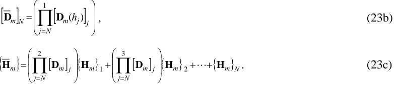
j, j=1, 2,…, N-1, (22)and then using Eqs.(21) and (22) recursively, a relationship between the state vectors
on the top and bottom surfaces of the laminate is established as follows:
{
Fm(hN)}
N=[ ]
DmN{
Fm(0)}
1+{ }
Hm , (23a)[ ]
[
( )]
1 ⎟ ⎟ ⎠ ⎞ ⎜ ⎜ ⎝ ⎛ =∏
=N j j j m Nm D h
D , (23b)
{ }
[ ]
{ }
[ ]
{ }
m{ }
m NN j j m m N j j m
m D H D H H
H ⎟⎟ + +
⎠ ⎞ ⎜ ⎜ ⎝ ⎛ + ⎟ ⎟ ⎠ ⎞ ⎜ ⎜ ⎝ ⎛ =
∏
∏
= = L 2 3 1 2. (23c)
{Fm(hN)}N and
{
Fm(0)}
1 are, respectively, the state vectors at the top and bottom surfacesof the laminated composite. The traction free conditions at the top and bottom
surfaces yields
[
] [
]
[
] [
]
⎪⎩ ⎪ ⎨ ⎧ = = T T N N m N m N m T T m m m h Z h Y h X Z Y X 0 0 0 ) ( ) ( ) ( 0 0 0 ) 0 ( ) 0 ( ) 0 (1 . (24)
Substituting Eq. (24) into Eq. (23) results in the following linear algebra equation
system ⎪ ⎭ ⎪ ⎬ ⎫ ⎪ ⎩ ⎪ ⎨ ⎧ − = ⎪ ⎭ ⎪ ⎬ ⎫ ⎪ ⎩ ⎪ ⎨ ⎧ ⎥ ⎥ ⎥ ⎦ ⎤ ⎢ ⎢ ⎢ ⎣ ⎡ 6 5 4 1 63 62 61 53 52 51 43 42 41 m m m m m m H H H W V U D D D D D D D D D
, (25)
where Dij and Hmi are the matrix elements in
[ ]
Dm and {Hm}of Eqs.(23b- 23c) that arerelated to the three displacement components at the bottom surface, respectively.
Eq.(25) is a set of linear algebra equations in terms of the three displacement
components, Um, Vm and Wm, at the top surface. The terms on the right-hand side of
Eq. (25), Hm4, Hm5 and Hm6, contain 4×N unknown constants,
− j
U , U+j , Vj−, and Vj+
(j=1, 2,…N), introduced in Eq.(19). Because of the continuity of U(0)(z) and V(0)(z) at
the interface between the jth and the (j+1)th sub-layers, 1
− +
+ =
j j U
U and 1
− +
+=
j j V
V (j=1,
2,…N-1). Hence, the number of unknown constants is then reduced to 2(N+1). These
constants are determined by introducing appropriate boundary conditions along the
transverse edges.
Ply-crack boundary conditions
When a general angle-ply laminate is subjected to an in-plane extension
perpendicular to the 90° fibers, transverse ply cracks appear parallel to the fibers and
across the entire width from edge to edge. For example, subject to a uniform biaxial
[image:11.595.92.483.75.160.2]extension, ε0 and F0, and a shear loading,S0, the [θ°m/90°n/φ°s] laminate shown in
denote the number of the real plies within a ply group. In reality, matrix cracks can
occur in any plies, but there are a large group of laminates, in which transverse
cracking in 90º plies is the dominated damage mode, and therefore the minor matrix
cracking in non-90º plies is ignored in the present model. Other damage modes, e.g.
delamination and fibre breakage usually occur at high crack densities, so the current
work focuses on low and intermediate crack densities.
Assuming that the cracks are equally spaced, a representative volume element
(Fig. 3) can be taken from any two neighboring cracks to predict the stress and
displacement fields.
For the cracked layers at x=0, L the boundary conditions are traction free,
i.e., σxx =σxy =0. For the un-cracked layers at x=0, L, due to the fact that the
laminate is subjected to uniform extension and shear loading, the displacements of an
uncracked layer in the x and y directions, u and v, remain constant, that is
⎩ ⎨ ⎧ = = 0 0 v ) z , y , 0 ( v u ) z , y , 0 ( u
. (26a)
Substituting Eq. (26a) and Eq. (14) into Eq. (5.13) yields at x=0 and y=0
⎪ ⎪ ⎩ ⎪ ⎪ ⎨ ⎧ = × ε + ⎟ ⎠ ⎞ ⎜ ⎝ ⎛ − × + × ξ = = ⎟ ⎠ ⎞ ⎜ ⎝ ⎛ − × + × ξ =
∑
∑
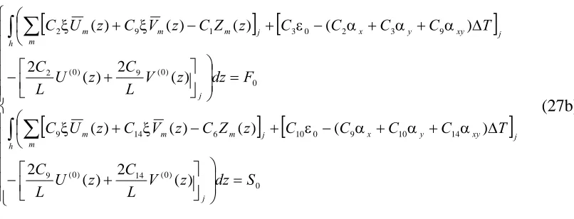
∞ = ∞ = 0 0 ) 0 ( 0 0 ) 0 ( 0 0 0 2 1 ) ( ) 0 sin( ) ( ) , 0 , 0 ( 0 2 1 ) ( ) 0 sin( ) ( ) , 0 , 0 ( v L z V z V z v u L z U z U z u m m m m (26b)From also the equilibrium of the internal and external forces, the following equation
exists ⎪ ⎪ ⎩ ⎪ ⎪ ⎨ ⎧ = =
∫
∫
h xy h xx S dz F dz 0 0 σ σ (27a)[
] [
]
[
] [
]
⎪ ⎪ ⎪ ⎪ ⎪ ⎪ ⎩ ⎪⎪ ⎪ ⎪ ⎪ ⎪ ⎨ ⎧ = ⎟ ⎟ ⎠ ⎞ ⎥⎦ ⎤ ⎢⎣ ⎡ + − ⎜ ⎝⎛ ξ + ξ − + ε − α + α + α Δ
= ⎟ ⎟ ⎠ ⎞ ⎥⎦ ⎤ ⎢⎣ ⎡ + − ⎜ ⎝
⎛ ξ + ξ − + ε − α + α + α Δ
∫ ∑
∫ ∑
0 ) 0 ( 14 ) 0 ( 9 14 10 9 0 10 6 14 9 0 ) 0 ( 9 ) 0 ( 2 9 3 2 0 3 1 9 2 ) ( 2 ) ( 2 ) ( ) ( ) ( ) ( ) ( 2 ) ( 2 ) ( ) ( ) ( ) ( S dz z V L C z U L C T C C C C z Z C z V C z U C F dz z V L C z U L C T C C C C z Z C z V C z U C j h j xy y x m j m m m j h j xy y x m j m m m (27b)where F0 and S0 are the forces per unit length (Fig. 3). From the introduction of the
boundary conditions, it can be seen that the solution can be found to the required
accuracy by increasing the total number of the thin layers.
Propagation of transverse cracking in laminates
[image:13.595.93.496.71.225.2]The total complementary potential energy of a representative element
Fig. 3 shows a representative volume element which is taken from between two
neighboring cracks in a [θ°m/90°n/φ°s] composite laminate. Assuming that stress
analysis has been carried out on this idealized element from the previous section,
where the laminate was assumed to consist of N fictitious sub-layers. By using the
present stress analysis, the total complementary potential energy is easier to obtain
than the total potential energy because the stresses, used to calculate the
complementary strain energy, are determined immediately after solving the state
space equations. The complementary strain energy Uc of this representative element is
∑
= = N j j c c U U 1 (28)where the superscript ‘j’ denotes the jth sub-layer and Ucj is the complementary strain
energy of the jth sub-layer of the representative volume element. Using the stresses
from the previous section, Ucj per unit length in the y direction can be obtained as
[
]
∫∫
σ ′ σ +Δ α σ= − j h L j T T j
c C T dxdz
U 0 0 1 } { } { } { ] [ } { 2 1 (29a) where T xy xz yz zz yy xx ] [ }
Considering that the laminate is under a uniformly prescribed strain ε0 in the y
direction, the potential of the prescribed strain ε0 can be calculated as
∑
= = N 1 jj c
c V
V
∑ ∫∫
[
]
=
= N
1 j
h
0 L
0 j
yy 0
j
dxdz
σ
ε (30)
The total complementary potential energy of this representative volume element is
given as the difference of the complementary strain energy Uc and the potential of
prescribed displacements Vc .
c
c V
U
Γ= −
∑ ∫∫
(
)
=
−
⎥⎦ ⎤ ⎢⎣
⎡ σ ′ σ +Δ α σ −ε σ
= N
j h L
j yy T
T
j
dxdz T
C 1 0 0
0 1
} { } { } { ] [ } { 2 1
(31)
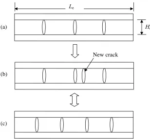
The energy release rate due to transverse cracking
Consider a composite laminate subjected to external loading and there are a
sufficiently large number of transverse cracks in the 90° layers. The entire length of
the laminate is Le and the thickness of cracked layers is Hc. Fig. 4 shows the
propagation process of the transverse cracks from state (a) to state (c). In state (a), it is
assumed that there exist k uniformly spaced transverse cracks in the laminate.
Therefore the crack density in this state is
e k
L k
= ρ
(32)
With the changes of external loading, a new transverse crack forms and the crack
pattern changes from state (a) to state (b). The number of the transverse cracks
increases from k to (k+1). Although in reality a new crack formation is randomly
distributed, the overall crack distribution tends to be uniform when the number of
cracks is large. In order to simplify the analysis, state (b) is idealized to state (c), in
which the (k+1) cracks are also equally spaced. The simplification of the crack
spacing here is also due to that the focus of the present study is the effect of crack
density on degradation of material properties. The crack density of state (c) is then
e k
L k 1
1
+ =
ρ + (33)
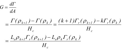
dA dΓ
G=
c
k r k e 1 k r 1 k e
c
k r 1
k r c
k 1
k
H
) ( L ) ( L
H
) ( k ) ( ) 1 k ( H
) ( ) (
ρ Γ ρ ρ
Γ ρ
ρ Γ ρ
Γ ρ
Γ ρ
Γ
− =
− +
= −
=
+ +
+ +
(34)
where Γ(ρk+1) and Γ(ρk) are the total complementary potential energies of the entire
laminate at crack densities ρk+1 and ρk , respectively; Γr(ρk+1) and Γr(ρk) are the
respective total complementary potential energies of the representative volume element at crack densities ρk+1 and ρk.
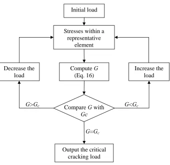
The transverse crack propagation criterion
A new crack will form if the energy released due to crack formation reaches
the critical energy release rate Gc, i.e.
c
G
G≥ (35)
Gc is a material property and has units of energy per unit area. It can be measured by
[image:15.595.147.406.71.179.2]an experimental method.
Fig. 5 is a flowchart showing how to determine the critical cracking load for a
given crack density. For a given load, stress analysis is carried out by using the state
space model. The energy release rate G of a representative volume element is then
computed by Eq. (34) and compared with Gc. If G>Gc, the current load is reduced to
achieve a smaller energy release rate until G=Gc. If G<Gc, the current load is
increased to obtain a larger energy release rate until G=Gc. If G=Gc, the current load
is taken as the critical cracking load for the given crack density.
Numerical results
The formulations and criterion proposed above are applied to predict transverse
cracking in composite laminates with different configurations, including symmetric
cross-ply laminates, symmetric angle-ply laminates and general non-symmetric
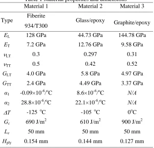
laminates. The material properties and dimension of these laminates (Liu and Nairn,
1992; Joffe et al., 2001) are given in Table 1. Effects of residual thermal stresses are
included in the analysis. ΔT is the difference between the room temperature and the
cure temperature. Table 1 also lists the critical energy release rate Gc for each
Symmetric laminates subjected to tension
The crack density as a function of applied average stresses for symmetric cross-ply
laminates is plotted in Fig.6. Herein, the applied average stress is the axial tension per
unit length in the x direction divided by the height H of the laminate. The test and
variational results of Liu and Narin (1992) are also shown in these figures for
comparisons. The numerical results for Material 1 with [0°2/90°2]s and [0°2/90°4]s
lamination profiles are plotted in Figs. 6a and 6b, respectively. Using a single value
of Gc, the predictions of the two laminates agree well with the experimental results,
which indicates that the critical energy release rate can be used as a material property
that characterizes transverse crack propagation in composite materials.
The dependence of crack density on the applied average stress for symmetric
angle-ply laminates with layups [±θ°/90°4]s are presented in Figs. 7a and 7b. The laminates
are composed of Material 2. The present results are compared with those obtained by
Monte-Carlo simulations and experimental data in Joffe et al. (2001). Once again very
good agreements are observed in these figures. It can be seen that cracks occur earlier
in the [±30°/90°4]s than in the [±15°/90°4]s laminates.
Non-symmetric laminates subjected to tension
After successful validation for cross-ply symmetric laminates, the method is applied
to predict transverse crack propagation in two non-symmetric laminates. The first one
is constructed by replacing one set of 90°4 layers in the above [±30°/90°4]s laminate
with 0°4 layers. Thus the new profile, [±30°/90°4/0°4/+30°], is now non-symmetric.
The stress-crack density relation of the non-symmetric laminate is plotted in Fig. 8a.
In comparison with Fig. 7b, the onset crack stress of the non-symmetric laminate is
significantly increased. The second laminate has a lay-up of [30°/90°/30°/90°] and is
composed of Material 3. Both the 90° layers are assumed to have transverse cracks
and the crack distributions in both layers are identical. Fig. 8b shows the crack density
as a function of the applied average stress in the laminate.
No comparisons have been made in Figs (8a) and (8b), because the present
solutions are believed to be the first ones in the literature on predicting transverse
Laminates subjected to tension and shearing
In this section, the present method is further used to study the effects of shearing on
transverse cracking. A symmetric and a non-symmetric cracked laminates under a
combination of tension and shearing are analyzed, respectively. It is assumed that the
laminates are composed of Material 3 from Table 1. A series of curves are shown in
Fig.9 to demonstrate the effects of shear stresses on the transverse cracking process of
a symmetric [30°/90°/90°/30°] laminate. The laminate is subjected to a combined
action of uniform tension and shearing. The applied average stress, which is the
average stress on the cross-section perpendicular to the x axis (Fig 2), increases, while
the shear stress keeps constant. The applied shear stresses are -100, -50, 0, 50 and 100
MPa, respectively. It can be seen that both the magnitude and the direction of shear
stresses have significant effect on the initiation and development of transverse cracks.
The negative shear stresses advance and the positive stresses delay the transverse
cracking. This is because the [30°/90°/90°/30°] laminate has a negative shear strain in
the x-y plane when the laminate is subjected to a single tension in the x direction (Fig
2). If a negative shear stress is also applied, the magnitude of the negative shear strain
increases. On the contrary, applying a positive shear stress decreases the magnitude of
the shear strain. As a result, the energy release rate in the case of applying negative
shear stress is higher than that in the cases of applying no shear stress or positive
stresses.
The same set of shear stresses are also applied on a non-symmetric
[30°/90°/30°/90°] laminate and the obtained stress-crack density relations are shown
in Fig. 10. As can be seen, the effect of shearing on cracking is similar to the
symmetric case. Nevertheless, under the same loading condition the crack initiation
stress of the non-symmetric laminate is slightly higher than that of the symmetric one.
This is because the 90° layers in the symmetric laminate are thicker and a thicker 90°
layer is more prone to crack formation.
To the authors’ best knowledge, comparable solutions to the results presented
in Figs. 9 and 10 are not available in the literature. The results can again be used as
benchmark solutions for future development of new theories.
By using the energy method, an approach based on the state space stress analysis to
predict the propagation of transverse cracking in general composite laminates has
been proposed. The proposed method inherits the advantages of the state space
method, by which an accurate stress distribution and, hence, an accurate estimate of
strain energy can be computed. The method can also deal with both symmetric and
non-symmetric laminates.
In conjunction with the stress analysis, the energy release rate due to
transverse cracking was derived in a laminate with an idealized uniform crack
distribution. A new crack forms when the energy release rate approaches the critical
energy release rate.
Numerical results for symmetric laminates were compared with alternative
numerical solutions and experimental results. The solution was extended to the
analysis of non-symmetric laminates under tension, and then to the analysis of general
laminates subjected to both tension and shearing. This provided new numerical
solutions that are hardly found in the literature. From the new results, it was found
that shearing had significant effect on the cracking process.
It is noted that in this work the transverse cracking process was simplified as a
crack density increment in a uniformly spaced state, while the nature of the crack
multiplication in reality is stochastic. Though good comparisons with test results have
been observed for the globe relationship between the applied stresses and crack
density, a statistical approach should be resorted to modeling transverse cracking in
future work in order to gain deeper understanding of the cracking process.
References
Bailey J E and Parvizi A 1981 On fiber debonding effects and the mechanism of tranverse-ply failure in cross-ply laminates of glass fiber/thermoset composites Journal of Materials Science 16 649-59
Dvorak G J and Laws N 1987 Analysis of progressive matrix cracking in composite laminates. II. First ply failure Journal of Composite Materials21 309-29
Fan J and Zhang J 1993 In-situ damage evolution and micro/macro transition for laminated composites Composites Science and Technology47 107
Flaggs D L and Kural M H 1982 Experimental determination of the in situ transverse lamina strength in graphite/epoxy laminates Journal of Composite Materials 16 103-16
Garrett K W and Bailey J E 1977 Multiple transverse fracture in 90o; cross-ply laminates of a glass fibre-reinforced polyester Journal of Materials Science12 157
Herakovich, C.T., 1998. Mechanics of fibrous composites. Wiley, New York.
Joffe R, Krasnikovs A and Varna J 2001 COD-based simulation of transverse
cracking and stiffness reduction in [θ/90n]s laminates Composites Science and
Technology61 637-56
Laws N and Dvorak G J 1988 Progressive transverse cracking in composite laminates Journal of Composite Materials22 900-16
Leblond P, El Mahi A and Berthelot J M 1996 2D and 3D numerical models of transverse cracking in cross-ply laminates Composites Science and Technology56 793
Lim S-H and Li S 2005 Energy release rates for transverse cracking and delaminations induced by transverse cracks in laminated composites Composites Part A (Applied Science and Manufacturing)36 1467-7
Liu S and Nairn J A 1992 The formation and propagation of matrix microcracks in cross-ply laminates during static loading Journal of Reinforced Plastics and Composites11 158-78
McCartney L N 1998 Predicting transverse crack formation in cross-ply laminates Composites Science and Technology58 1069-81
McCartney L N 2000 Model to predict effects of triaxial loading on ply cracking in general symmetric laminates Composites Science and Technology60 2255
McCartney L N 2004 Effect of mixed mode loading on ply crack development in laminated composites: theory and application. Nat. Phys. Lab., Teddington, UK) p iv+22
McCartney L N 2005 Energy-based prediction of progressive ply cracking and strength of general symmetric laminates using an homogenisation method Composites Part A (Applied Science and Manufacturing)36 119-28
Nairn J A 1989 The strain energy release rate of composite microcracking: a variational approach Journal of Composite Materials23 1106
Nairn J A 2000 Comprehensive Composite Materials, ed Z Anthony Kelly and Carl (Oxford: Pergamon) p 403
Nairn J A, Hu S and Bark J S 1993 A critical evaluation of theories for predicting microcracking in composite laminates Journal of Materials Science28 5099-111
Parvizi A, Garrett K W and Bailey J E 1978 Constrained cracking in glass fibre-reinforced epoxy cross-ply laminates Journal of Materials Science13 195-201
Sirivedin S, Fenner D N, Nath R B and Galiotis C 2006 Viscoplastic finite element analysis of matrix crack propagation in model continuous-carbon fibre/epoxy composites Composites Part A: Applied Science and Manufacturing37 1922-35
Smith P A and Ogin S L 1999 On transverse matrix cracking in cross-ply laminates loaded in simple bending Composites - Part A: Applied Science and
Manufacturing30 1003.
Soldatos, K.P. and Ye, J.Q. (1994). Wave propagation in anisotropic laminated hollow cylinders of infinite extent. Journal of Acoustics Society of America. 96(5), Part I, 3744-3752.
Wang A S D, Kishore N N and Li C A 1985 Crack development in graphite-epoxy cross-ply laminates under uniaxial tension Composites Science and
Technology24 1
Ye J Q 2002 Laminated Composite Plates and shells: 3D Modelling (London: Springer)
Ye J Q and Sheng H Y 2003 Free-edge effect in cross-ply laminated hollow cylinders subjected to axisymmetric transverse loads International Journal of
Mechanical Sciences45 1309-26
Ye J Q, Sheng H Y and Qin Q H 2004 A state space finite element for laminated composites with free edges and subjected to transverse and in-plane loads. Computers and Structures82(15/16) 1131-1141.
Ye J Q and Soldatos K P 1994a Three-dimensional stress analysis of orthotropic and cross-ply laminated hollow cylinders and cylindrical panels Computer Methods in Applied Mechanics and Engineering117 331-51
Ye J Q and Soldatos K P 1994b Three-dimensional vibration of laminated cylinders and cylindrical panels with symmetric or antisymmetric cross-ply lay-up Composites Engineering4 429-44
Ye J Q and Soldatos K P 1995 Three-dimensional buckling analysis of laminated composite hollow cylinders and cylindrical panels International Journal of Solids and Structures32 1949-62
Yokozeki T, Aoki T and Ishikawa T 2002 Transverse crack propagation in the specimen width direction of CFRP laminates under static tensile loadings Journal of Composite Materials36 2085
Yokozeki T, Aoki T and Ishikawa T 2005 Consecutive matrix cracking in contiguous plies of composite laminates International Journal of Solids and Structures42 2785
Zhang J, Fan J and Soutis C 1992 Analysis of multiple matrix cracking in [±θm/90n]s
composite laminates. 1. In-plane stiffness properties Composites23 291.
Zhang D, Ye J Q and Lam D 2007a Free-edge and Ply Cracking Effect in Angle-ply Laminated Composites subjected to In-plane Loads Journal of Engineering Mechanics, Transactions ASCE 133(12) 1268-1277.
Table 1 Material properties and dimensions
Material 1 Material 2 Material 3
Type Fiberite 934/T300
Glass/epoxy Graphite/epoxy
EL 128 GPa 44.73 GPa 144.78 GPa
ET 7.2 GPa 12.76 GPa 9.58 GPa
νLT 0.3 0.297 0.31
νTT 0.5 0.42 0.52
GLT 4.0 GPa 5.8 GPa 4.97 GPa
GTT 2.4 GPa 4.49 GPa 3.37 GPa
α1 -0.09×10⁻⁶/oC 8.6×10⁻⁶/oC N/A α2 28.8×10⁻⁶/oC 22.1×10⁻⁶/oC N/A
ΔT -125 oC -105 oC 0oC
Gc 690 J/m2 610 J/m2 900 J/m2
Le 50 mm 50 mm 50 mm
Fig. 1 Nomenclature of an off-axis lamina.
θ
0
ε
0
ε
L 2
1
h
Z, 3 X
[image:23.595.156.405.76.236.2]Fig. 2 Schematic view of a [θ°m/90°n/φ°s] laminate with an array of transverse ply
cracks in 90°n layers.
L
H 0
ε
0 ε
F0 F0
S0 S0
X Y
Z
θ°m
90°n
Fig. 3 A representative volume element of a [θ°m/90°n/φ°s] laminate with ply cracks in
90°n layers.
θ°m
90°n
φ°s X
Z
L
Fig. 4 Nomenclature of the propagation process of transverse cracks and the idealised uniform distribution state.
Hc
New crack (a)
(b)
(c)
Fig. 5. Flowchart of calculating critical cracking load for a given crack density.
G>Gc
Stresses within a representative
element
G=Gc
Output the critical cracking load Decrease the
load
Initial load
Compute G (Eq. 16)
Compare G with Gc
Increase the load
0 0.2 0.4 0.6 0.8 1
400 600 800 1000 1200 1400 1600
Applied Average Stress (MPa)
Cr
ack Densi
ty (
1
/m
m
)
Present
Variational Method Experimental Data `
0 0.2 0.4 0.6 0.8
200 400 600 800 1000 1200
Applied Average Stress (MPa)
C
rack D
ensi
ty
(1
/m
m
)
Present
Variational Method
Experimental Data `
[image:28.595.95.487.73.254.2](a) (b)
Fig. 6 Dependence of crack density on the applied average stress in (a) Fiberite 934/T300 [0°2/90°2]s laminate with transverse cracks.
0 0.1 0.2 0.3 0.4 0.5 0.6
100 150 200 250 300 350
Applied Average Stress (MPa)
Cr
ack Densi
ty
(
1
/m
m
)
Present
Monte-Carlo Simulation Experimental Data `
0 0.1 0.2 0.3 0.4 0.5 0.6
100 125 150 175 200 225 250
Applied Average Stress (MPa)
C
rack D
ensi
ty (
1
/m
m
)
Present
Monte-Carlo Simulation Experimental Data `
[image:29.595.97.497.72.251.2](a) (b)
Fig. 7 Dependence of crack density on the applied average stress in (a) [±15°/90°4]s glass/epoxy laminate with transverse cracks.
0 0.1 0.2 0.3 0.4 0.5 0.6
300 350 400 450 500
Applied Average Stress (MPa)
C
rack D
ensi
ty (
1
/m
m
)
Present `
0 0.3 0.6 0.9 1.2 1.5
200 300 400 500 600
Applied Average Stress (MPa)
Cr
a
ck
De
n
si
ty
(
1
/m
m
)
Present `
[image:30.595.96.490.73.238.2](a) (b)
Fig. 8. Dependence of crack density on the applied average stress in
(a) [±30°/90°4/0°4/+30°] glass/epoxy laminate with transverse cracks;
0 0.3 0.6 0.9 1.2 1.5
0 100 200 300 400 500 600 700 800
Applied Average Stress (MPa)
C
ra
ck D
e
nsi
ty (
1
/m
m
)
`
Fig.9. Dependence of crack density on the applied average stress and shear stresses in a [30°/90°/90°/30°] graphite/epoxy laminate.
xy
σ
=-100MPaxy
σ
=-50MPaxy
σ
=0MPaxy
σ
=50MPaxy
0 0.3 0.6 0.9 1.2 1.5
0 100 200 300 400 500 600 700 800
Applied Average Stress (MPa)
C
ra
ck D
e
n
si
ty (
1
/m
m
)
`
Fig.10. Dependence of crack density on the applied average stress and shear stresses in a [30°/90°/30°/90°] graphite/epoxy laminate.
xy
σ
=-100MPaxy
σ
=-50MPaxy
σ
=0MPaxy
σ
=50MPaxy

![Fig. 2 Schematic view of a [θ°m/90°n/φ°s] laminate with an array of transverse ply cracks in 90°n layers](https://thumb-us.123doks.com/thumbv2/123dok_us/8005639.210182/24.595.163.395.93.198/fig-schematic-view-laminate-array-transverse-cracks-layers.webp)
![Fig. 3 A representative volume element of a [θ°m/90°n/φ°s] laminate with ply cracks in 90°n layers](https://thumb-us.123doks.com/thumbv2/123dok_us/8005639.210182/25.595.187.416.92.194/fig-representative-volume-element-laminate-ply-cracks-layers.webp)
![Fig. 6 Dependence of crack density on the applied average stress in (a) Fiberite 934/T300 [0°2/90°2]s laminate with transverse cracks](https://thumb-us.123doks.com/thumbv2/123dok_us/8005639.210182/28.595.95.487.73.254/dependence-density-applied-average-stress-fiberite-laminate-transverse.webp)
