RIT Scholar Works
Theses Thesis/Dissertation Collections
5-1-1980
Comparison of the derivative-transform edge
gradient analysis technique to tatian's method of
edge gradient analysis, varying random noise,
truncation interval and sampling internal on
analytical edges
Robert LaFlesh
Follow this and additional works at:http://scholarworks.rit.edu/theses
This Thesis is brought to you for free and open access by the Thesis/Dissertation Collections at RIT Scholar Works. It has been accepted for inclusion in Theses by an authorized administrator of RIT Scholar Works. For more information, please [email protected].
Recommended Citation
ANALYSIS TECHNIQUE TO TATIAN'S mETHOD OF EDGE GRADIENT
ANALYSIS, VARYING RANDom NOISE, TRUNCATION INTERVAL
AND SAmPLING INTERVAL ON ANALYTICAL EDGES
by
Robert B~ LaFlesh
A thesis submitted in partial fulfillment of the requirements for the degree of Bachelor of Science in the School of Photographic Arts and Sciences in the College of Graphic Arts and Photography of the Rochester Institute of Technology
may, 1980
Signature of the Author •••••••••••••••••••••••••••••••••• Photographic Science
and Instrumentation
Certified
Accepted
by ••••••••••••••••••••••••••••••••••••••••••••• Thesis Adviser
COMPARISON OF THE DERIVATIVE-TRANSFORM EDGE GRADIENT ANALYSIS TECHNIQUE TO TATIAN'S METHOD OF EDGE GRADIENT ANALYSIS, VARYING RANDom NOISE, TRUNCATION INTERVAL
AND SAMPLING INTERVAL aN ANALYTICAL EDGES
by
Robert B. LaFlesh
Sumitted to the
Photographic Science and Instrumentation Division in partial fulfillment of the requirements
for the Bachelor of Science degree at the Rochester Institute of Technology
ABSTRACT
The following work has been computer simulated.
A cumulative gaussian step response and the step response of a photographic emulsion 1 were taken through the
derivative-transform edge gradient analysis technique and Tatian's method of analysis. Random noise levels, truncation intervals and sampling intervals on the
analytic edges were varied to determine their influence on each technique. The variance and means of the cal-culated m.T.F.s were then statistically tested for no difference of the two techniques. The exact noise free M.T.F. was also calculated and compared to the M.T.F.s calculated by the two techniques. The results show a statistical difference in the two techniques at low
frequencies. This difference was deemed not significant from a practical standpoint because the magnitude of the differences between the M.T.F.s was small compared to the actual magnitude of the M.T.F.s at low frequencies. Also the two techniques produced M.T.F.s of high devia-~ tions from the exact noise free transform at high
frequencies ..
The author wishes to extend his graditude to his
thesis advisor Mr. Roland 'JJ. Porth of the Xerox
Coroora-tion for suggesting the original topic of study and for
the numerous interesting and informative talks of imag
ing science that lead to the culmination of this thesis,
Also the author wishes to thank Dr. Newburg of the
Rochester Institute of Technology for his mathematical
aid in the thesis work.
Finally a special thanks to Mr. Dan Siems and
Mr. Tim Wilson, students of the Rochester Institute of
Technology, for their computer expertise which was
extremely helpful while programming.
LIST OF FIGURES ...vi
LIST OF TABLES ix
INTRODUCTION 1
THEORETICAL BACKGROUND 3
HYPOTHESES , 11
PROCEDURE 12
DISCUSSION ..25
RECOMMENDATIONS 37
SUMMARY 38
REFERENCES 40
APPENDIX A: GRAPHICAL DATA OUTPUT 42
APPENDIX B: MAIN PROGRAMS 67
FDATA 68
GADATA 69
DERIV 70
DTRANS , 71
TATIAN 73
MAIN1 75
MAIN2 ,76
MAIN2P 77
MAIN3 78
DIFF 82
TESTVAR 83
TESTMEAN 84
APPENDIX C: GRAPHING PROGRAMS 85
GRAPH2 .86
GRAPHDIFF 8 8
FGRAPH1T 90
FGRAPH2T 92
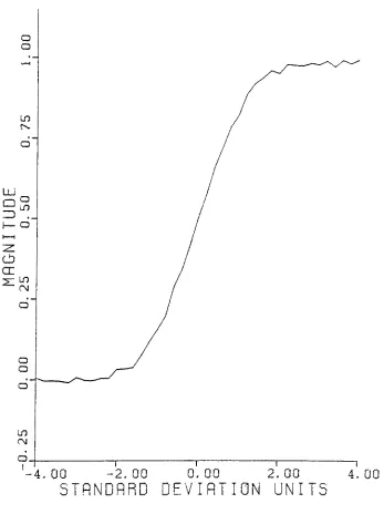
FIGURE 1: EDGE UJITH 100:1 SIGNALtNOISE RATIO
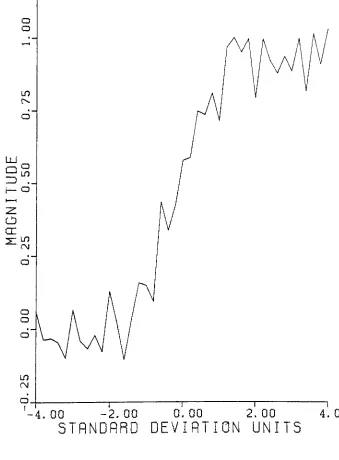
FIGURE 2: EDGE WITH 100:10 SIGNALrNOISE RATIO
FIGURE 3: GRAPHICAL DATA GENERATING PROCEDURE
FIGURE 4: GRAPHICAL DATA GENERATING PROCEDURE
FIGURE 5: m.T.F.COMPARISON OF GAUSSIAN SPRD. FCTN. M.T.F.=AVERAGE OF 1000 M.T.F.S
10:1 (SIGNALtNOISE) 5.333 (SAMPLES/SIGMA )
FIGURE 6: M.T.F.COMPARISON OF GAUSSIAN SPRD. FCTN. M.T.F.sAVERAGE OF 1000 M.T.F.S
10:1 (SIGNAL :NOISE) 1 . 333(SAMPLES7SIGMA )
FIGURE 7: DIFFERENCE OF M.T.F . (-)CONTINUOUS TRANSFORM OF GAUSSIAN SPRD. FCTN. VARYING S I GNAL:NOISE(DERV.-TRANSFORM)
FIGURE 8: DIFFERENCE OF M.T.F. (-)CONTINUOUS TRANSFORM OF GAUSSIAN SPRD. FCTN. VARYING SIGNAL:NOISE(TATIAN)
FIGURE 9: M.T.F. OF GAUSSIAN SPRD. FCTN. VARYING SIGNALrNOISE RATIO(TATIAN )
FIGURE 10: VARIANCE OF GAUSSIAN SPRD. FCTN. VARYING SIGNALrNOISE RATIO(TATIAN)
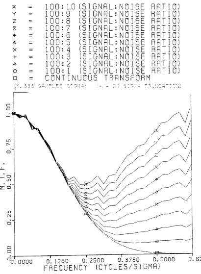
FTGURE 11: M.T.F. OF GAUSSIAN SPRD. FCTN. VARYING SIGNALrNOISE RAT10(DERV.-TRANSFORM)
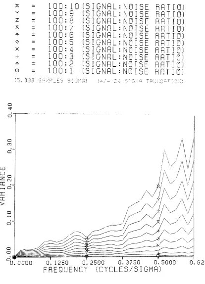
FIGURE 12: VARIANCE OF GAUSSIAN SPRD. FCTN. VARYING SIGNALrNOISE RATIO(DERV.-TRANSFORM)
FIGURE 13: M.T^F. OF__GAUSSIAN SPRD. FCTN. VARYING SAMPLING INTERVAL(TATIAN)
FIGURE 14: VARIANCE OF GAUSSIAN SPRD. FCTN. VARYING SAMPLING INTERVAL(TATIAN)
FIGURE 15: M.T.F. OF GAUSSIAN SPRD. FCTN. VARYING SAMPLING INTERVAL (DERV.-TRANSFORM)
FIGURE 17: M.T.F. OF GAUSSIAN SPRD. FCTN. VARYING TRUNCATION INTERVAL (TATIAN )
FIGURE 18: VARIANCE OF GAUSSIAN SPRD. FCTN. VARYING TRUNCATION INTERVA L(TATIAN)
FIGURE 19: M.T.F. OF GAUSSIAN SPRD. FCTN. VARYING TRUNCATION INTERVAL(DERV--TRANSFORM)
FIGURE 20: VARIANCE OF GAUSSIAN SPRD. FCTN. VARYING TRUNCATION INTERVAL (DERV--TRANSFORM)
FIGURE 21: M.T.F. OF FRIESER SPRD. FCTN. VARYING SIGNALrNOISE RATIO(TATIAN )
FIGURE 22: VARIANCE OF FRIESER SPRD. FCTN. VARYING SIGNALrNOISE RATIO(TATIAN )
FIGURE 23: M.T.F. OF FRIESER SPRD. FCTN. VARYING SIGNALrNOISE RATIO(DERV.-TRANSFORM)
FIGURE 24: VARIANCE OF FRIESER SPRD. FCTN. VARYING
SIGNALrNOISE RATIO(DERV.-TRANSFORM)
FIGURE 25r M.T.F. OF FRIESER SPRD. FCTN. VARYING SAMPLING INTERVAL(TATIAN)
FIGURE 26: VARIANCE OF FRIESER SPRD. FCTN. VARYING SAMPLING INTERVAL(TATIAN)
FIGURE 27: M.T.F. OF FRIESER SPRD. FCTN. VARYING SAMPLING INTERVAL (DERV.-TRANSFORM)
FIGURE 28: VARIANCE OF FRIESER SPRD. FCTN. VARYING SAMPLING INTERVAL (DERV.-TRANSFORM)
FIGURE 29: M.T.F. OF FRIESER SPRD. FCTN. VARYING TRUNCATION INTERVAL (TATIAN )
FIGURE 30: VARIANCE OF FRIESER SPRD. FCTN. VARYING TRUNCATION INTERVAL (TATIAN )
FIGURE 31: M.T.F. OF FRIESER SPRD. FCTN. VARYING TRUNCATION INTERVAL(DERV.-TRANSFORM)
TABLE 1: STATISTICALLY SIGNIFICANT DIFFERENT MEANS
TABLE 2r STATISTICALLY SIGNIFICANT DIFFERENT VARIANCES
TABLE 3: STATISTICALLY SIGNIFICANT DIFFERENT VARIANCES
Generating the line spread function by taking the
numerical derivative of the edge response function will 2
magnify the effects of noise. Tatians direct method of
reduction of the edge response function avoids the diff
icultly of taking the numerical derivative of a noisy
3
function. The influence of noise, in theory, is thought
to be quite complex and was therefore not attempted in
4
this paper. Therefore noise was only used as a black
box system to determine if a difference exist between
the final output of Tatian's technique and the deriva
tive-transform technique of edge analysis.
The truncation interval and the sampling interval
also effect the accuracy of the M.T.F. due to the in
herent nature of the theory of Fourier algebra. By
varying these parameters of noise, truncation and
sampling intervals, a comparison was made to determine the usefullness of either technique.
Most edge analysis systems operate on Tatian's
technique of edge gradient analysis,, But from the theo
retical standpoint both methods are the same. There
purpose of this research is to determine if a difference
exist between the two techniques while using a computer
Since edges occur frequently in nature they are
readily available for a method of system analysis. The theory of edge analysis begins with an object. First
the object f(?) is divided into infinitely long rect angles of width d?. The intensity of one of the sub
divisions of the object is f(i)dl. The image of each of
the subdivisions is a line spread function. Therefore the line spread function h(\) is an image of a line object formed by a system.
If g(x) is the image irradiance, then dg(x) is the
image irradiance at the point x due to the subdivisions
of the object at I . Therefore 4}Cx) =
?(*)V.(x-*}<U
(D
If the point x is held fixed and the irradiance
contributions are summed for all oossible object sub
divisions, the total image irradiance at x will be ob
tained. This is accomolished by integrating equation 1
over all possible values of \\ . The image irradiance at
x, g(x ) is then
*(!>H*-T)d5
convolution is
4
*
*.(*)
i-^T.
An edge can now be considered the object. For a
unit edge f(S)=0.0 for?<-0.0 and f(*)=1.0 forl^O.O.
Since f(I) * h(5) = h(I ) * f(l)
Since the edge represents a step function
X
(4)
where e(x) is the image irradiance. Graphically
e(x}
* 'I
The edge image irradiance is just the
cumulative area
under the spread function
I.V\A&E Of DC>E.
Differentiating equation 4
..<<.
-Ujtt aC*)
Equation 5 is one of the basic equations of
system
The O.T.F. is defined as the Fourier
-oo (6) Substituting equation 5 into equation 6 yields
dx
ao dx (?j
In practice an edge is scanned on a microdensitometer
which yields density or transmittance vs. position. This
curve is then converted from density or transmittance vs.
position to effective exposure vs. position using the
7
macroscopic response curve.
The derivative-transform technique of edge analysis
makes use of equation 7 in the following way. The num
erical derivative of the edge irradiance(effective
exposure) is taken to approximate the line spread function
of the system. The Fast Fourier transform is then
applied which produces the O.T.F..
Tatian's method of edge analysis makes use of the
fact that the numerical derivative of a function f(x) in
the spatial domain is equal to multiplying the functions
transform F(s), frequency representation of f(x), by
i2-fff. This is represented by 8
V
dx (8)where
-UTT-fx
e(x) e dx , ECO
(10)
Equation 10 is Tatian's derivation of the O.T.F.. In
terms of sampled values of the edge response function
the O.T.F. is given by10
X
L2Trfe0i}c0
-L.2Tr-?y..i
(Hi
>?0
(n)This applies only where the line spread function
h(x) is band limited, i.e. its transform vanishes for
frequencies greater than a cutoff frequency f ; and the
sample space obeys the conditiont=.-=^f .
To obtain a working formula Tatian truncated the
infinite limits of equation 11 and added correction
factors. These correction factors are based on the
1 -i
asymptotic behavior of e(x). Since the transfer func
tion of photographic film is sought only two correction
factors are derived for the working formula. The
deriva-1 2 tion of these correction factors are as follows
It is known that
x
e(x) =
(
K(1)U/-ao
(4)
which equals
(12) for a unit edge
o f(l)=0.0 for?<.0.0
"c
Substituting equation 13 into equation 12
Changing the order of integration
Taking the transform of the step function
Expanding and making use of the sifting property
(14)
(15)
(16)
fM-^T.W-^XCfl +
lT^f^
IT-?"""
2TT-f
>
(17)
The integral of an odd function over symetric limits
equals zero. Therefore
(18)
Since T(f) is the transform of a real function, T<|(f)
and T2(f) are even and odd functions, respectively.
Therefore equation 18 can be written
Vj r
2TTf
+
T.Cfl
cos2trf
2TTf
u
(19)The behavior of e(n ) for large n, (spatial domain), 11
depends on that of T(f) near its origin. Expanding
n yields
e(ne) ss l*
T*
Coy
_ T/"^) 2TT**e 2$or Uf^e n (20)
(-no * -xl -Tree), ....
Since T.,(f) is an even function and T2(f) is an odd
function all of the coefficients T '(0), T '''(0), ....
and Tj'^O), ... would be zero if T(f) were an analytic
function at the origin. The even and odd parts of e(x)
are given by
(21)
(22)
'2
Substituting equation 20 into equation 21 yields
ea(n-) *, O +
Tt
(o)/2TTan.i
Note that since analytic edges were compared in this
technique
very close to one and e(-nfe) is very close to zero.
Equation 11 can be written in its even and odd parts as
oo
n-\
(24)
I. ns,
-The values of e (ne) and e2(ne) in equation 24 can be
given in terms of actual sampled values only up to some
finite value of n, say N. For n larger than N, e.(nfe)
and e-,(ne) are given by equation 23. Breaking down
equation 24 yields
N 1
T(fl.HWt
[*!?!
t,Me-2f* t|,Mc*2^1(25)
Substituting equation 23 into equation 24 and making use
of the relationships
.V*i
a^Cu^
(26)^K1
COT IAU = -SiryC-^ *^U
yields
-p- pV / W
-3TT -P 4.
Cos(N*V^aiT^
T,
27)Tatian's method is exact when the sum is carried to
an infinite scan length. The truncation required by
Tatian's algorithm(finite scan length) produces error.
HYPOTHESES
The purpose of this experiment is to determine if
there is no difference between Tatian's method of edge
gradient analysis and the derivative-transform technique
of edge analysis. The factors that will be varied are
the level of random noise, truncation interval and the
sampling interval of the edge.
The hypotheses to be tested are
There is no significant difference between the variances
of the calculated M.T.F.s using Tatian's vs. the deriv
ative-transform edge analysis technique
and,
there is no significant difference between the means of
the calculated M.T.F.s using Tatian's vs. the
derivative-transform edge analysis technique.
Fisher (F) tests will test for no significant diff
erence of variances at various frequencies. T tests will
test for no significant difference of means at various
PROCEDURE
All of the data required for this analysis was
15
computer simulated. The entire program analysis was
broken down into many subroutines and mini-programs which allowed a variety of functions to be included in any one
run of the program. It was also considered by the
exper-imentor to be the most systematic way of developing the program. Four subroutines by other authors were used.
1(S
They were the Fortran subroutine FOURG by Norman Brenner
to calculate Fast Fourier Transforms, subroutines GAUSS
1 7
and RANDU which together compute normally distributed
1 fl
uncorrelated random numbers with a given mean and 1 9
standard deviation and the subroutine NTDR for gen erating the cumulative gaussian edge.
The computer program GADATA, to generate the anal
ytic cumulative gaussian curve, was produced first. The
cumulative gaussian curve is given by
t%3
'-an
dx
This curve was choosen because it approximates a cum ulative photographic system spread function. A normal
interval could be produced in terms of standard deviation
units, <T .
A subroutine of Tatian's method, TATIAN, equation
27, was then created to produce the M.T.F. and Phase
angle in radians of the input edge function.
A subroutine of the derivative-transform method,
DTRANS and supporting subroutine DERIV, representing
equation 7,within finite limits, were then created to
produce the M.T.F. and Phase in radians of the input
edge data.
Four main programs were developed next to produce
an average M.T.F. of the M.T.F.s calculated by DTRANS
and TATIAN while varying levels of random noise, MAIN1;
varying sampling interval, MAIN2 and MAIN2P; and varying
truncation interval, MAIN3.
MAIN1 calculated an average M.T.F. and correspond
ing variances at the following signalrnoise ratios
100:10 100:5
100:9 100:4
100:8 100:3
100:7 100:2
100:6 100:1
Signalrnoise ratio was defined to be the maximum signal
level divided by the standard deviation of the noise,
in Figure 1 and 2.
The systematic flow of generating an average M.T.F.
and its variances for different levels of random noise
was as follows
An analytic edge with values between zero and one,
inclusive, corresponding to
+/-24T, was created by
GADATA. This edge had a samoling interval of 5.333
samples/ty. This edge was then read into MAIN1. A cer
tain level of random noise that was independent of signal
level was then added to the edge* The noisy edge was
then taken through both TATIAN and DTRANS to produce two
M.T.F.s. This process, of adding the same level of
random noise to the edge and taking it through both
TATIAN and DTRANS(with constant samoling and truncation
intervals) was repeated one hundred times to produce two
families of curves, one family for each M.T.F. method.
The mean and variance, at different frequencies, of each
family of curves was then determined in MAIN1 to produce
an average M.T.F. and corresponding variances. This
entire procedure was repeated for the ten afore-mentioned
different levels of random noise. This yielded the first
row of Figure 3.
MAIN2 and MAIN2P calculated an average M.T.F. and
variances at the sampling interval corresponding to the
ratio of the edges were 20:1 with a +/- 24
T truncation
interval. MAIN2 read five different sets of edge data
with sampling interval
5.333 samples/T
4.500
samples/g-3.458 samples/j
2.417
samples/g-1 . 333 samples/r
MAIN2P read only one set of edge data for each run. Two
runs were made with samoling intervals
.667 samples/ir
.333 samples/V
The systematic flow of generating an average M.T.F.
and variances for different sampling intervals was as
follows
The seven analytic edges of varying sampling interval
were created by GADATA. These edges were read inta their
perspective programs, MAIN2 or MAIN2P. A .05 level of
random noise was added over each of the differently
sampled edges. This is representative of a 20:1 signal:
noise ratio with +/- 24 <T truncation interval. Each
noisy edge was then taken through both TATIAN and DTRANS
to produce forteen M.T.F.s. This process of adding the
same level of random noise to each differently samoled
(with constant truncation interval and constant level
of random noise) was repeated one hundred times for each
differently sampled edge to produce forteen families of
curves, one family for each M.T.F. method with each
different sampling interval. The mean and variance, at
different frequencies, of each family of curves was then
determined in MAIN2 and MAIN2P to produce an average
M.T.F. and corresponding variances. This process yielded
the second row of Figure 3.
MAIN3 calculated an average M.T.F. and variances
at the following truncation intervals
+/- 5.0625 <T ?/- 2.8125 CT
+/-.5625 CT
?/- 2.4375 V
?/- 2.0625 IT
+/- 1.6875 <T
+/- 1.3125 T
+/-.9375 1
The systematic flow of generating average M.T.F.s
and variances for different truncation intervals was as
follows
An analytic edge with values between zero and one, inclusive, corresponding to
+/- 24
<T, was created by
GADATA. The sampling interval of this edge was kept
a
constant 5.333 samoles/<T. This original
edge was read
into MAIN3. A .05 level of random
noise was added to ?/- 4.6875 CT
+/- 4.3125
Q-?/- 3.9375 <T
?/- 3.5625 H
+/- 3.1875
0-the points on the edge inbetween the truncation points.
The noisy edge was then taken through both TATIAN and
DTRANS to produce two M.T.F.s. This process of adding
the same level of random noise to the edge and taking it
through both TATIAN and DTRANS(with constant sampling
interval and constant level of random noise) was repeated
one hundred times to produce two families of curves, one
family for each M.T.F. method. The mean and variances,
at different frequencies, of each family of curves was
then determined in MAIN3 to produce an average M.T.F.
and corresponding variances. This procedure was then
repeated for different truncation intervals. The trun
cation segment of MAIN3 became active after the first
average M.T.F. and variances were determined. The
original analytic edge data was truncated by setting
ooints outside and including the required truncation
points to zero and one D.C. levels. This procedure
represents a truncated edge which was truncated at exact
ly the required points. The truncation interval on the
analytic edge decreased in units of
+/-.3750 <T after
each average M.T.F. and variances were determined. The
afore-mentioned truncation intervals were thus produced.
This process yielded the third row of Figure 3.
The computer program FDATA, to generate the analytic
cumulative Frieser curve, was produced next.
cumulative Frieser curve is given by
This curve was choosen because it approximates a cumula
tive photographic emulsion spread function. A normalized
Frieser curve was used so that sampling and truncation
intervals could be produced in terms of standard deviation
units, <r.
The main program MAIN1 read the cumulative Frieser
analytic edge. This edge had a sampling interval of
5.333 samples/tj-. The systematic flow of generating an
average M.T.F. and variances for different levels of
random noise followed the afore-mentioned procedure of
MAIN1. This yielded the first row of Figure 4.
The main programs MAIN2 and MAIN2P read the cumula
tive Frieser analytic edges where the sampling intervals
were similiar to the previous procedure of MAIN2 and
MAIN2P. The systematic flow of generating an average
M.T.F. and variances for different sampling intervals
followed the afore-mentioned procedure of MAIN2 and
MAIN2P. This yielded the second row of Figure 4.
The main program FMAIN3 was developed to produce an
average M.T.F. of the M.T.F.s calculated by TATIAN and
DTRANS while varying truncation interval. FMAIN3
+/- 13.3125 <T
+/- 12.7500 <r
+/-12.1875 Q
+/- 11
.6250 <r
->/- 11.0625 0*
?/- 10.5000 0"
+/-9.9375 <T
+/- 4.3125 cr
+/- 3.7500 <T
+/- 3.1875 tr
+/- 2.6250 V
+/- 2.0625 <T
+/- 1
.5000 T
+/-.9375 <T following truncation intervals of the input edge data
?/- 13,8750 Q"
+/- 9.3750 V ?/_ 4.8750CT
+/- 9.8125 0*
>/- 8.2500 ff
+/- 7.6875 CT
+/- 7.12 50 cr
+/- 6.5625 T
+/- 6.0000 cr
?/- 5.4375 <T
The main program FMAIN3 read the cumulative Frieser
analytic edge as the original edge data0
The systematic flow of generating average M.T.F.s
and variances for different truncation intervals was the
same as that of MAIN3. The only difference in the two
programs was that FMAIN3 decreased its truncation interval
of the Frieser analytic edge in units of
>/-.5625 CT
after each average M.T.F. and variances were determined.
This yielded the third row of Figure 4.
The number of tuncation intervals for both cumula
tive edges was choosen on the basis of an upper limit of
computer central processing unit time for each individual
run of MAIN3 or FMAIN3. The limit was set to approx
imately twenty minutes.
The program TESTVAR was developed to test the input
statistic was the larger sample variance/smaller sample
variance. The program output the significantly different
variances and the test statistic.
The program TESTMEAN was developed to determine the
test statistic and degrees of freedom of the input means
at a .1 level of confidence using an approximation of the
20 Fisher-Behrens test
A series of graphing programs, for the Zeta plotting
system21, to be used for specific graphing purposes were
developed last for data output and data comparison.
These programs were
GRAPH XGRAPH2T FGRAPH1D
GRAPH2 XGRAPH2D FGRAPH2T
GRAPHDIFF XGRAPH3T FGRAPH2D
XGRAPH1T XGRAPH3D FGRAPH3T
XGRAPH1D FGRAPH1T FGRAPH3D
A representative group of these programs can be found
in
appendix C of this thesis with their specific
purpose
'-4. 00 -2. 00 0. 00 2. 00
STRNDRRD DEVIATION UNITS
4. 00
FIGURE 1 :
[image:31.564.94.441.180.644.2]'-4. 00 -2.00 0.00 2.00
STANDRRD DEVIATION UNITS
4. 00
FIGURE 2:
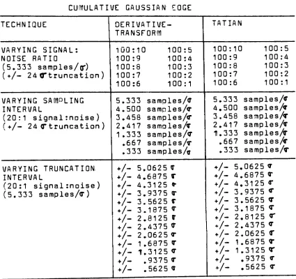
[image:32.564.91.430.195.655.2]CUMULATIVE GAUSSIAN EDGE
TECHNIQUE DERIVATIVE- TATIAN
TRANSFORM
VARYING SIGNAL: 100: 10 100:5 100: 10 100:5
NOISE RATIO 100:9 100:4 100: 9 I00r4
(5.333 samples/or) 100: 8 100:3 100: 8 I00r3
( +/- 24 (Ttruncation
) 100: 7 100:2 100' 7 100:2 100'
6 100:1 100 6 100:1
VARYING SAMPLING 5.333 samples/tT 5.333 samples/cr
INTERVAL 4.500 samples/* 4.500 samples/*
(20:1 signal:noise ) 3.458 samples/* 3.458 samples/r
(+/- 24 (Ttruncation) 2.417 samDles/ff 2.417 samples/*
1 .333 samples/tT 1.333 samples/*
.667 samples/* .667 samples/* .333 samples/^ .333 samples/*
VARYING TRUNCATION ?/- 5.0625 T
+/r 5.0625 *
INTERVAL ?/- 4.6875 * +/- 4.6875 *
(20:1 signal :noise ) */- 4.3125
t-+/r
4.3125 * (5.333 samples/*) ?/- 3.9375 * +/r 3.93750*
*/- 3.5625 * */- 3.5625 T ?/- 3.1875 <T ?/- 3.1875 T
+/- 2.8125 "
?/- 2.8125 <T
+/- 2.4375 0"
+/- 2.4375 cr +/- 2.0625 * ?/,- 2.0625 CT ?/- 1.6875 *
+/r 1.6875 *
?/- 1.3125 cr ?/- 1.3125 cr
+/- .9375 *
+^- .9375 *
?/- .5625 *
+/- .5625 *
FIGURE 3:
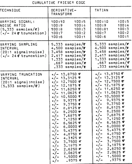
[image:33.564.68.493.73.473.2]CUMULATIVE FRIESER EDGE TECHNIQUE DERIVATIVE-TRANSFORM TATIAN VARYING SIGNAL: NOISE RATIO (5.333 samoles/*)
(+/- 24 <r truncation )
100r10 100:9 100:8 100:7 100:6 100:5 100:4 100:3 100:2 100:1 100:10 100:9 100:81 100:7 100:6 100:5 100:4 100:3 100:2 100:1 VARYING SAMPLING INTERVAL
(20:1 signal:noise )
(+/- 24 CT truncation )
5.333 4.500 3.458 2.417 1.333 .667 .333 samples/cr samples/* samples/* samples/* samples/* samples/* samples/* 5.333 samples/* 4.500 samples/* 3.458 samples/* 2.417 samples/* 1.333 samples/* .667 samples/* .333 samples/* VARYING TRUNCATION INTERVAL
(20:1 signal :noise )
(5.333 samples/cr)
?/- 13.8750 *
?/- 13.3125 *
?/- 12.7500 <r ?/- 12.1875 * +/- 11
.6250 *
?/- 11 .0625 *
?/- 10.5000 * ?/- 9.9375 CT
?/- 9.3750 *
?/- 8.ei25 <r
?/- 8.2500 **
+/- 7.6875 *
?/- 7.1250 *
+/- 6.5625 *
?/- 6.0000 *
?/- 5.4375 * ?/- 4.8750 * ?/- 4.3125 * ?/- 3.7500 *
+/- 3.1875 <r
?/- 2.6250 V ?/- 2o0625<r ?/- 1.5000 * +/- .9375 *
?/-!
I
::
t-i
3.8750 * 3.3125 * 2.7500 2.1875 1.6250 1.0625 0.5000 9.9375 9.3750 8.8125 8.2500 7.6875 7.1250 6.5625 6.0000 5.4375 4.8750 4.3125 3.7500 3.1875 2.6250 2.0625 1 .5000 .9375 cr * * * * * tr r * * <T *" cr cr * * * cr * * FIGURE 4: [image:34.564.69.494.73.600.2]DISCUSSION
The results of the test on the means and variances
are tabulated in Tables 1,2 and 3.
The variability of obtaining M.T.F.s from Tatian's
technique and the derivative-transform technique while
varying truncation interval on both the Frieser and the
Gaussian cumulative edge curves, at the sampling interval
of 5.333 samples/* and signalrnoise ratio of 20:1, are
the same. The Fisher-Behrens test of the means has
shown that there is no difference in calculating M.T.F.
values from Tatian's technique and the
derivative-transform technique while varying the truncation interval
on both the Frieser and Gaussian cumulative edge curves,
at the sampling interval of 5.333 samples/* and 20:1
signal:noise ratio. This sampling interval places approx
imately thirty two points on the edge where the edge
contains 99.72^ of its unit area.
The variability of obtaining M.T.F.s from Tatian's
technique and the derivative-transform technique while
varying the signal:noise ratios on both the Frieser and
the Gaussian cumulative edge curves, at the sampling
+/- 24<T
are not the same at low frequencies. This
difference in the variances in the two techniques can
possibly be attributed to how each technique handles the
noise. The different variances occured at the low
frequencies of approximately .0208 through .1458 cycles/cr.
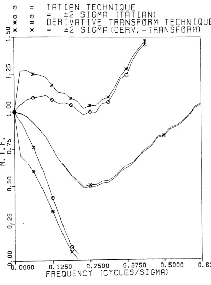
This corresponds to an error free M.T.F. in the range of
1.0 through .65. Tatian's technique produced lower
variances at these frequencies by an approximate 1 :2
ratio. Figures 5 and 6 demonstrate the difference in
the variances of the two techniques at low frequencies.
It can also be noted that as the level of random noise
decreases the higher of the low frequencies, of different
variability, began to have the same variability. This
adds to the idea that the difference between the var
iances of the two techniques exist because of how each
technique handles the noise. The higher the noise the
more variability between the two techniques. The
Fisher-Behrens test of the means has shown that there is no
difference in calculating the M.T.F. values from Tatian's
technique to the derivative-transform technique while
varying the signalrnoise ratio on both the Frieser and
the Gaussian cumulative edge curves, at the samoling
interval of 5.333 and truncation interval
of +/- 24CT.
technique and the derivative-transform technique while
varying the sampling interval on both the Frieser and
the Gaussian cumulative edge curves, at a 20:1 signal:
noise ratio with a
+/-24CT truncation interval, are not
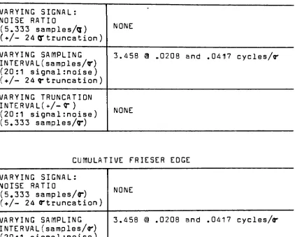
the same at low frequencies. The Fisher-Behrens test of
the means has shown that there is a difference in calcul
ating M.T.F. values, at low frequencies, from Tatian's
technique and the derivative-transform technique while
varying the sampling interval on both the Frieser and the
Gaussian cumulative edge curves, at a 20:1 signal:noise
ratio with a +/- 24 CT truncation
interval. This differ
ence in the means occured at the sampling interval of
3.458 samples/cr for both the Frieser and the Gaussian
cumulative edge curves. Since this occured in the low
frequencies it is believed to be attributed to how each
technique handles the noise. This is based on the
significantly different variances that were observed
in the low frequencies during the test of the variances.
The deviation of Tatian's and the
derivative-transform technique from the continuous noise free
transform is graphed in Figures 7 and 8, respectively.
These represent varying signal:noise ratios on the
cumulative gaussian edge.
General remarks are also to be noted in the graph
fluctuations occurs with increasing frequency. An in
crease in fluctuations occurs with increasing sampling
interval at constant truncation interval. Also servers
truncation causes deformation of the output M.T.F..
This graphical data output is located in appendix A.
A very important topic that must be discussed for
these results to apply to the practical world is
normalization. Normalization, after transformation of
the line spread function, was not required in this study
of the derivative-transform technique, because the
original edge data was assumed to run from zero to one
D.C. levels. It is important to note that the
pre-normalization of the edge data is not necessary for the
derivativetransform technique in actual practice, as
long as the resulting M.T.F. is properly normalized.
Pre-normalization of the original edge data is
manditory in Tatian's technique. Since there is no
central ordinate value of the M.T.F. produced by Tatian's
technique, it is not possible to properly normalize the
data after the M.T.F. is obtained, by division of each
value by the central ordinate M.T.F. value. Therefore
in practice the edge data must be pre-normalized to run
from zero to one D.C. levels. The decision is left to
the reader to sacrifice the variability of Tatian's
pre-normalize the edge data for the derivative-transform
technique.
Most of the differences between the means and
variances, in the data, occured at low frequencies rel
ative to the M.T.F. 's folding frequency values. The
significantly different variances were approximately
.005 or less in most cases. The
significantly different
means were approximately equal to 1.0.
From the practical standpoint the error produced by
using either technique is relatively small when the
actual magnitude of the M.T.F. values are compared to
the magnitude of the statistically significant variance
values. Therefore these statistically different mean
TABLE 1:
STATISTICALLY SIGNIFICANT DIFFERENT MEANS
CUMULATIVE GAUSSIAN EDGE
VARYING SIGNAL: NOISE RATIO
(5.333 samples/d) (+/- 24 CT truncation
)
NONE
VARYING SAMPLING
INTERVAL(samples/cr)
(20:1 signal :noise )
(+/- 24
cj-truncation)
3.458 a .0208 and .0417 cycles/*
VARYING TRUNCATION
INTERVAL(+/-Q" )
(20:1 signal :noise )
(5.333 samples/cr)
NONE
CUMULATIVE FRIESER EDGE
VARYING SIGNAL: NOISE RATIO
(5.333 samples/r) (?/- 24 trtruncation )
NONE
VARYING SAMPLING INTERVAL(samples/<r) (20:1 signalrnoise) (+/- 24 *truncation )
3.458 @ .0208 and .0417
cycles/**
VARYING TRUNCATION
INTERVAL^/- *)
(20:1 signal:noise )
(5.333 samples/*)
[image:40.564.70.492.151.491.2]TABLE 2:
STATISTICALLY SIGNIFICANT DIFFERENT VARIANCES
CUMULATIVE GAUSSIAN EDGE
VARYING SIGNAL: NOISE
(5.333 samples/*)
(?/- 24 CT truncation
)
100:10 @ .0208 through .1458 cycles/fr
100:9 @ .0208 through .1458 cycles/*
100:8 a .0208 through .1458 cycles/*
100:7 @ .0208 through .1458 cycles/v
100:6 a .0208 through .1458 cycles/*
100:5 d .0208 through .1458 cycles/^
100:4 @ .0208 through .1458 cycles/r
100:3 I .0208 through .1458 cycles/*
100:2 Q .0208 through .1250 cycles/*
100:1 a .0208 through .1250 cycles/*
VARYING SAMPLING
INTERVAL(samples/*)
(20:1 signal :noise )
(+/- 24 C truncation)
5.333 @ .0208 through .1458 cycles/*
4.500 ! ,,0208 through .1250 cycles/*
3.458 .0208 through .1250 cycles/*
2.417 9 .0208 through .1042 cycles/*
1.333 a .020B through .0625 cycles/r
.667 tl .0208 and 90417 cycles/*
.333 ta .0208 cycles/
VARYING TRUNCATION
INTERVAL^/- * )
(20:1 signalrnoise)
(5.333 samples/*)
TABLE 3:
STATISTICALLY SIGNIFICANT DIFFERENT VARIANCES
CUMULATIVE FRIESER EDGE
VARYING SIGNAL: NOISE RATIO
(5.333 samples/cr)
(+/- 24 (Ttruncation )
100:10 a .0208 through
100:9 a .0208 through
100:8 .0208 through
100:7 ti .0208 through
100:6 8 .0208 through
100:5 (a .0208 through
100:4 @ .0208 through
100:3 t .0208 through
100:2 e .0208 through
100:1 @ .0208 through
.1458 cycles/*
.1458 cycles/*
,1458 cycles/*
.1458 cycles,*
.1458 cycles/r
.1458 cycles/<r
.1458 cycles/*
.1250 cycles/*
.1250 cycles/*
.1250 cycles/*
VARYING SAMPLING INTERVAL(samples/cT)
(20:1 signalrnoise)
(+/- 24 (Ttruncation)
5.333 1 .0208 through .1458 cycles/*
4.500 d .0208 through .1250 cycles/*
3.458 ti .0208 through .1250 cycles/*
2.417 ta .0208 through .1042 cycles/*
1.333 9 .0208 through .0833 cycles/r
.667 @ .0208 and .0417 cycles/*
.333 @ .0208 cycles/*
VARYING TRUNCATION
INTERVAL(+/~ <T)
(20:1 signal :noise)
(5.333 samples/*)
O
o
*
* *
TRTIRN TECHNIQUE
= 2 SIGMA (TATIAN)
DERIVATIVE TRANSFORM TECHNIQUE
= 2 SIGMA (DERV.
-TRANSFORM)
^.0000 0 1250 0.2500 0.3750 0.5000
FREQUENCY (CYCLES/SIGMA)
0. 6250
FIGURE 5:
Ml .F. COMPARISON OF
GAUSSIRN SPRD. FCTN
MTF =AVERAGE OF 1000 M.T.F.S
[image:43.564.70.482.66.623.2]o in
* -=
* *
TATIAN
TECHNIQUE
=2 SIGMA (TATIAN)
DERIVATIVE
TRANSFORM
TECHNIQUE= 2
SIGMA (DERV. -TRANSFORM)
O. 0000 0.1250 0.2500 0.3750 0.5000
FREQUENCY (CYCLES/SIGMA)
0. 6250
M
f
F COMPARISON OF GAUSSIAN SPRD. FCTN.M. T. F. =AVERAGE OF 1000 M.T.F.S
W Y Z X + o X + 100 100 100 100 100 100 100 100 100 100 10 (SIGNAL 9 (SIGNAL 8 (SIGNAL 7 (SIGNAL 6 (SIGNAL 5 (SIGNAL 4 (SIGNAL 3 (SIGNAL 2 (SIGNAL 1 (SIGNAL NOI NQI NOI NOI NOI NOI NOI NOI NOI NQI E E E E E E E E E E RR RR RR RR RR RR RR RR RR RR TIO) TIO) TIO) TIO) TIO) TIO) TIO) TIO) TIO) TIO) TRUNCATION") t r
0 1250 0.2500 0.3750 0.5000 0.6250
FREQUENCY (CYCLES/SIGMA)
DIFFERENCE OF M.T.F. (-) CONT I NUOUS
TRANSFORM OF GRUSSIRN SPRD. FCTN.
Y
Z
X
X
+
A
o
100: 10 (SIGNRL
100:9 (SIGNRL 100:8 (SIGNRL 100:7 (SIGNRL 100:6 (SIGNRL 100:5 (SIGNRL 100:4 (SIGNRL 100:3 (SIGNRL 100:2 (SIGNAL 100:1 (SIGNAL
NOISE NOISE NOISE NOISE NOISE NOISE NOISE NOISE NOISE NOISE
RATIO) RATIO) RATIO) RATIO) RATIO)
RATIO) RATIO) RATIO) RATIO) RATIO)
0. 0000 0.1250 0.2500 0.3750 0.5000
FREQUENCY (CYCLES/SIGMA)
0. 6250
DIFFERENCE OF M.T.F. (-) CONT I NUOUS
TRANSFORM OF GAUSSIAN SPRD. FCTN.
RECOMMENDATIONS
A possible avenue for future work is an analytic
study of Tatian's technique compared to the
derivative-transform technique which would provide the reason for
the statistical difference in M.T.F.s at low frequencies,
Another prospect could be formed by comparing the
two techniques using signal dependent noise which re
SUMMARY
Two subroutines, TATIAN and DTRANS, were built to
be the fundamental data generating sources. TATIAN
determined the M.T.F. of the input curve by Tatian's
method of edge gradient analysis. This consisted of
taking an F.F.T. of the original edge data, multiplying
by i2Tff and then applying Tatian's correction factors.
DTRANS determined the M.T.F. of the input curve by the
derivative-transform technique which consisted of taking
the numerical derivative of the original edge data to
approximate the line spread function, and then performing
an F.F.T. which produced the M.T.F.
A series of main programs, MAIN1, MAIN2, MAIN2P,
MAIN3, FMAIN3, produced average M.T.F.s and corresoonding
variances. The statistical tests, of the mean (TESTMEAN ) ,
and variances (TESTVAR) , were then run to analyze the data
and test the hypotheses.
The variability of the calculated M.T.F.s using
Tatian's technique vs. the derivative-transform edge
analysis technique were differant at low frequencies.
Also the calculated mean M.T.F.s using Tatian's technique
low frequencies when a sampling interval of 3.458
samples/CJ was tested. This sampling interval corresponds
to approximately 21 points on the edge where 99.72$ of
REFERENCES
1. H.F.Gilmore, 0. Opt. Soc. Am. 57,75 (1967)
2. M.E.Rabedeau, J. Opt. Soc. Am. 59,1309 (1969)
3. B.Tatian, 0. Opt. Soc. Am. 61, 1223 (1971)
4. Ibid., 1223 (1971)
5. Private communication with R.Porth
6. O.Carson, Supplementary lecture notes, Rochester Institute of Technology, p. 5-7 (1977)
7. 3.C.Dainty, R.Shaw, Image Science, Academic Press, N.Y. p.245
8. R. Bracewell, The Fourier Transform and Its Applica
tions. McGraw-Hill, U.S. (1978) p. 117
9. B.Tatian, 0. Opt. Sac. Am. 55, 1015 (1965)
10. Ibid. , p.1016
11. Ibid., p. 1016
12. Ibid., p. 1014-1017
13. R.Barakat, ft.Houston, 0. Opt. Soc. Am. 53, 1244(1963)
14. D.Dutton, Applied Optics 14, 515 (1975)
15. Xerox Sigma Nine main frame computer, DEC 11/34
Intelligent Remote Batch Terminal and peripherals,
ROSS User Computing Center, Rochester Institute of
Technology
16. N.Brenner, M.I.T. Lincoln Lab, 9/12/68
17. I.B.M. Scientific Subroutine Package
19. I.B.M. Scientific Subroutine Package
20. A.Rickmers, H.Todd, Statistics An Introduction,
McGraw-Hill, U.S. p. 119 (1967)
21. Zeta Incremental Plotting System, Zeta 3600s
plotter with attached PDP11/04KA controller and a
1600 BPI tape drive, ROSS User Computing Center,
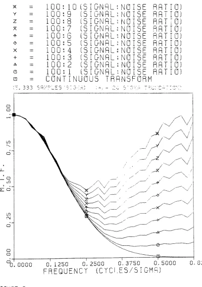
X Y Z X + X + A CD 100 100 100 100 100 100 100 100 100 100 10 9 8 7 6 5 4 3 2 1 CONTI (SIGNAL (SIGNAL (SIGNAL (SIGNAL (SIGNAL (SIGNAL (SIGNAL (SIGNAL (SIGNAL (SIGNAL UOUS TR NO IS
- NO IS
'
NOIS
- NO IS
. NOIS i NOIS -NOIS i NOIS NQIS NOIS ANSFQ E E E E E E E E E E RM. RA RA RA RA RA RA RA RA RA RA TIO) TIO) TIO) TIQJ TIO) TIO) TIG) TIG) TIO) TIO)
cQ;,'
r.-0. 0000 0. 1250 0. 2500
FREQUENCY CCYCI
0,3750 0,5000
FS/SIGMA)
0. 5250
FIGURE 9:
M. T. F. SIGNAL
OF GAUSSIAN SPRD, NOISE RATIO (TATIA )
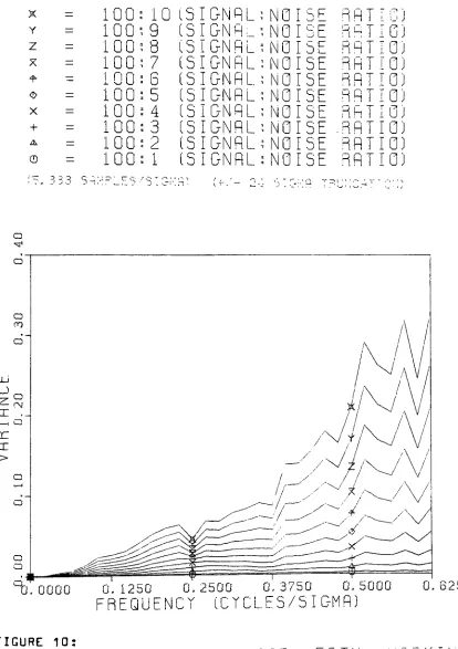
[image:53.564.73.481.69.648.2]X Y Z X X + A
100 : 10 100:9 100:8 100 s 7 100 100 100 100 100 100 6 5 4 3 2 1 (SIGNRL (SIGNAL (SIGNAL (SIGNAL (SIGNAL (SIGNAL (SIGNAL (SIGNAL (SIGNAL (SIGNAL NOISE NOISE NOISE NOISE NOISE NOIS^ i_ NOISE NOISE NOISE NOISE RAT RAT RAT RAT RAT RAT HhT RAT RAT RAT IC) 10) 10) 10) 10) 10) 10) 10) 10) 10)
0. 0000 0 1250 0,2500 0,3750 0,5000 0. B250 FREQUENCY (CYCLES/SIGMA)
FIGURE 10:
VARIANCE QF GAUSSIAN SPRD. SIGNALRNOISE RATIO (TATIAN)
[image:54.564.74.488.70.657.2]X Y X X + A 100: 10 100:9 100:8 100:7 100:6 100:5 100: 4 100:3 100:2 100: 1 CONTIN . iZ'..*-' aT c, 'Q"; (SIGNAL (SIGNAL (SIGNAL (SIGNAL (SIGNAL (SIGNAL (SIGNAL (SIGNAL (SIGNAL (SIGNAL UOUS TR NOI NQI NOI NQI NOI :NOIS :NQIS :NQIS :NOIS :NQIS ANSFQ E E E E E E E E E E RM RA RA RA RA RA RA RA RA RA RA TIO) TIO) TIO) TIO) TIO) TIO) TIO) TIO) TIO) TIO)
"0. 0000 0.1250 0.2500 0.3750 0.5000
FREQUENCY (CYCLES/SIGMA)
0. 6250
figure 11:
GRUSStrn s p p, Q FCTN. VARYING
[image:55.564.72.482.69.628.2]X
Y
X
X
+
A
o
100 100 100 100 100 100 100 100 100
100: 1
10 (SIGNAL 9 (SIGNAL 8 (SIGNAL (SIGNAL (SIGNAL (SIGNAL (SIGNAL (SIGNAL (SIGNAL (SIGNAL 7
6 5 4 3 2
NOISE NOISE NOISE NOISE NOISE NOISE NOISE NOISE NOISE NOISE
RATIO) RATIO) RATIO) RATIO) RATIO) RATIO) RATIO) RATIO) RATIO) RATIO) 333
o
0. 0000 0.1250 0.2500 0.3750 0.5000
FREQUENCY (CYCLES/SIGMA)
0. 6250
FIGURE 12:
VARIANCE OF GAUSSIAN SPRD. FCTN. VARYING
[image:56.564.73.487.68.642.2]A
+
X
X
m
5. 4 3 2 1
333 500 458 417 333 667 333
(SAMPLES/SIGMA) (SAMPLES/SIGMA) (SAMPLES/SIGMA) (SAMPLES/SIGMA) (SAMPLES/SIGMA) (SAMPLES/SIGMA) (SAMPLES/S IGMA) CONTINUOUS TRANSFORM
0, 0000 0.1250 0.2500 0.3750 0.5000
FREQUENCY (CYCLES/SIGMA)
0. 6250
A
+
X
X
5
4
3 2
1
333 500 458
417
333 667 333
(SAMPL (SAMPL (SAMPL (SAMPL (SAMPL (SAMPL (SAMPL
ES/S ES/S ES/S ES/S ES/S ES/S ES/S
IGMA) IGMA)
IGMA) IGMA)
IGMA) IGMA)
IGMA)
SE.
o
atf
0, 0000 0.1250 0.2500 0,3750 0,5000
FREQUENCY (CYCLES/SIGMA)
0, 6250
FIGURE 14:
VARIANCE OF GAUSSIAN SPriD, FCT
SAMPLING INTERVAL (TATIRN)
[image:58.564.71.491.75.659.2]A
T
X
X
a
5. 333
4, 500 3. 458
2, 417
1. 3
(SAMPLES/SIGMA) (SAMPLES/SIGMA) (SAMPLES/SIGMA) (SAMPLES/SIGMA) (SAMPLES/SIGMA)
. 667 (SAMPLES/SIGMA)
. 333 (SAMPLES/SIGMA)
CONTINUOUS TRANSFORM
ir1
1_ !:oi J i_j ..+/ tL.- -i i- ,n i
QQ O ^
O,
0. 0000 0.1250 0.2500 0.3750 0.5000 FREQUENCY (CYCLES/SIGMA)
0. 6250
F I GURE 15*
M T F
'OF
GAUSSIAN SPRD. FCTN. VARYINGO
A
+
X
X
5. 4. 3. 2, 1.
333 500 458
417
333 667 333
(SAMP (SAMP (SAMP (SAMP
LES/S
LES/S LES/S LES/S
(SAMPLES/S (SAMPLES/S (SAMPLES/S
IGMA)
IGMA)
IGMA)
IGMA)
IGMA) IGMA) IGMA)
:"-:T^F \
o
"TJ. 0000 0.1250 0.2500 0.3750 0.5000
FREQUENCY (CYCLES/SIGMA)
0. 6250
FIGURE 16:
VARIANCE OF GAUSSIAN SPRD, FCTN, VARYING
[image:60.564.76.493.74.637.2]X
+
ffl
. 9375 SIGMA 1. 3125 SIGMA 1. 6875 SIGMA 2, 0625 SIGMA 5, 0625 SIGMA
CONTINUOUS TRANSFORM
D: c-:;
Cb. oooo 0,1250 0.2500 0.3750 0.5000
FREQUENCY (CYCLES/SIGMA)
0, 6250
M^tV^QF GAUSSIAN SPRD, FCTN, VARYING
<!>
X
+
A =
=
=
s:c-::jl
- 9375 SIGMA
1= 3125 SIGMA 1= 6875 SIGMA
2, 0625 SIGMA 3, 9375 SIGMA
5, 0625 SIGMA
333 ''
tr c <*
--J O.
0. 0000 0.1250 0.2500 0.3750 0,5000
FREQUENCY (CYCLES/SIGMA)
0,6250
VF^Ufy&t OF GAUSSIAN SPRD, FCT
TRUNCATION I NTERV AL (T AT I AN)
L-o
X
+
+
, 9375 SIGMA
1. 3125 SIGMA
1, 6875 SIGMA
2, 0625 SIGMA
5. 0625 SIGMA
CONTINUOUS TRANSFORM
0. 0000 0.1250 0.2500 0.3750 0.5000
FREQUENCY (CYCLES/SIGMA)
0. 6250
rtcijpr 19
M. T. F. OF GAUSSIAN SPRD, FCTN, VARYING
O
X
I
T
A
. 9375 SIGMA
1, 3125 SIGMA 1. 6875 SIGMA 2, 0625 SIGMA
3. 9375 SIGMA 5, 0625 SIGMA
333 . _i;/d
'
crc.
0. 0000 0. 1250 0. 2500 0.3750 0.5000 FREQUENCY (CYCLES/SIGMA)
0. 6250
^PJA^CE
OF GAUSSIAN SPRD, FCTN, VARYINGx Y Z X X + A a 'A 100 100 100 100 100 100 100 100 100 100 10 9 8 7 6 5 4 3 2 1 CQNTI (SIGNAL (SIGNAL (SIGNAL (SIGNAL (SIGNAL (SIGNAL (SIGNAL (SIGNAL (SIGNAL (SIGNAL UQUS TR . NOISE : NQISE :NQISE : NOISE NOISE :NOISE : NOISE :NOISE :NOISE : NOISE ANSFQR RAT RAT RAT RAT RAT RAT RAT RAT RAT RAT 10) 10) 10) 10) 10) 10) 10) 10) 10) 10) M
0. 0000 0 1250 0,2500 0.3750 0,5000
FREQUENCY (CYCLES/SIGMA)
0. 6250
ricuRE 2i:
FRIE5ER spRD. FCTN
SIGNRL-NOISE RATIO(TATIAN)
Y
Z
X
4-<L>
X
+
A
100:
100:
100:
100: 100: 100:
100:
100: 100: 100:
n1
fl.es.
10 (SIGNAL 9 (SIGNAL
8 (SIGNAL
7 (SIGNAL
6 (SIGNAL
5 (SIGNAL 4 (SIGNAL
3 (SIGNAL
2 (SIGNAL 1 (SIGNAL
NOISE RATIO)
NOISE RATIO)
NOISE RATIO)
NOISE RATIO)
NOISE RATIO)
NOISE RATIO)
NOISE RATIO) NOISE RATIO)
NOISE RATIO) NOISE RATIO)
0. 0000 0 1250 0.2500 0.3750 0,5000 0.6250
FREQUENCY (CYCLES/SIGMA)
F I GURE 22 *
VARIANCE OF FRIESER SPRD
SIGNALrNOISE RATIO (ThTiAN
X
Y
Z
X
o
X
+
A
o
m
100: 10
(SIGNAL:N0ISE
RATIO)100:9
(SIGNAL:NOISE
RATIO) 100:8(SIGNAL:NQISE
RATIO) 100:7(SIGNAL:NOISE
RATIO) 100:6 (SIGNAL: NOISE RATIO) 100:5(SIGNAL:NOISE
RATIO) 100:4(SIGNAL:NOISE
RATIO) 100:3 (SIGNAL: NOISE RATIO) 100:2(SIGNAL:NOISE
RATIO)100: 1
(SIGNAL:NQISE
RATIO)CONTINUOUS TRANSFORM
Q,
0.0000 0.1250 0.2500 0.3750 0.5000
FREQUENCY ."CYCLES/SIGMA)
0. 6250
FIGURE 23:
[image:67.564.76.488.72.645.2]X
Y
~7
X
X
+
A
100: 10 (SIGNAL: NQISF RATIO)
100:9
(SIGNAL-NOISE
RATIO) 100:8(SIGNAL:NOISE
RATIO) 100:7(SIGNAL:NQISE
RATIO)100:6
(SIGNAL:NOISE
RATIO) 100:5(SIGNAL:NOISE
RATIO) 100:4 (SIGNAL: NOISE RATIO)100:3
(SIGNAL:NOISE
RATIO) 100:2 (SIGNAL: NOISE RATIO)100: 1
(SIGNAL:NOISE
RATIO)I'D)
0. 0000 0.1250 0.2500 0.3750 0.5000
FREQUENCY (CYCLES/SIGMA)
0. 6250
FIGURE 24:
VARIANCE OF FRIESER SPRD, FCTN. VARYING
[image:68.564.72.477.76.636.2]~z 5, 333
A -= 4, 500
+ = 3, 458
X = 2. 417
<!> = 1. 333
+ =
. 667
X =
. 333
m = CQNTI
(SAMPLES/SIGMA)
(SAMPLES/SIGMA)
(SAMPLES/SIGMA) (SAMPLES/SIGMA) (SAMPLES/SIGMA) (SAMPLES/SIGMA) (SAMPLES/SIGMA)NUQUS TRANSFORM
s:
^.0000
0.1250 0.2500 0.3750 0.5000FREQUENCY (CYCLES/SIGMA)
0. 6250
FIGURE 25:
M T F OF FRIESER SPRD, FCTN, VARYING
[image:69.564.70.492.68.644.2]A
+
X
X
5,
4,
3, 2. 1.
333 500 458
417
333 667 333
.;oise.
(SAMP (SAMP (SAMP (SAMP (SAMP (SAMP (SAMP
LES/S
LES/S
LES/S LES/S LES/S LES/S LES/S
IGMA) IGMA) IGMA) IGMA) IGMA) IGMA) IGMA)
o
cb.
oooo 0.1250 0.2500 0.3750 0.5000 FREQUENCY (CYCLES/SIGMA)0. 6250
FIGURE 26:
VARIANCE OF FRIESER SPRD, FCTN, VARYING
[image:70.564.70.490.78.650.2]A
+
X
X
m
5,333 (SAMPLES/S
4, 500 (SAMPLES/S
3. 458 (SAMPLES/S
2,417 (SAMPLES/S
1.333 (SAMPLES/S
. 667 (SAMPLES/S
(SAMPLES/S INUOUS TRANS CON
q33
IGMA)
IGMA)
IGMA) IGMA) IGMA)
IGMA) IGMA) FORM
0. 0000 0 1250 0.2500 0.3750 0.5000
FREQUENCY (CYCLES/SIGMA)
0. 6250
FTTHRF 9 7
MTF
'OF
FRIESER SPRD. FCTN. VARYINGo = 5, 333
A 4,
500
+ 3. 458
X rr 2, 417
<L> = 1
- do
j
*
. 667
X rr
. 333
(SAMPLES/SIGMA)
(SAMPLES/SIGMA)
(SAMPLES/SIGMA)
(SAMPLES/SIGMA)
(SAMPLES/SIGMR)
(SAMPLES/SIGMA)
(SAMPLES/SIGMA)
s"g:'L'
0. 0000 0.1250 0.2500 0.3750 0.5000
FREQUENCY (CYCLES/SIGMA)
0. 6250
FIGURE 28:
[image:72.564.74.492.70.643.2]Y
Z
X
+
1, 2, 2,
8,
13,
CON
+
: i 3 . L--I.H_
'
9375 SIGMA
5000 SIGMA
0625 SIGMA
6250 SIGMA
1875 SIGMA
8125 SIGMA
8750 SIGMA
TINUOUS TRANSFORM
j.Oi_i '.0. 3j^i jnr llj, Oii;"!.-..
O,
0. 0000 0 1250 0. 2500 0.3750 0,5000 FREQUENCY (CYCLES/SIGMA)
0, 6250
MICtV9V FRIESER SPRD, FCTN, VARYING
Y
Z
X
X
+
A
o
C-l
LO
LU
CJ
yZ.
CT
i i
QC cr
o
+
+
. 9375
1, 5000
2, 0625
2, 6250
3. 1875
6, 0000
8, 8125
11, 6250
13, 8750
SIGMA SIGMA SIGMA SIGMA SIGMA
SIGMA SIGMA SIGMA SIGMA
--- -WIa.
/ V /
0, 0000 0 1250 0,2500 0,3750 0.5000
FREQUENCY (CYCLES/SIGMA)
0. 6250
F I GURE 30 *
VARIANCE OF FRIESER SPRD, FCT
TRUNCATION INTERVAL (TATiAN)
Y
Z
X
+
CD
. 9375 SIGMA
1. 5000 SIGMA 2. 0625 SIGMA 2, 6250 SIGMA 3. 1875 SIGMA 8, 8125 SIGMA
13. 8750 SIGMA
CONTINUOUS TRANSFORM
sio;:-: I SE ;c;-'
-?' .L.3
0. 0000 0 1250 0.2500 0.3750 0.5000
FREQUENCY (CYCLES/SIGMA)
0. 6250
rt pi
ipc-31
MTF OF FRIESER SPRD, FCTN, VARYING
Y
Z
X
4>
<r>
x
+
A
1 2 2, 3,
+
6, 8.
1 1.
13.
9375
5000
0625
6250 1875 0000 8125 6250 8750
SIGMA SIGMA SIGMA SIGMA
IGMA
IGMA
IGMA IGMA
SIGMA
TJ. 0000 0.1250 0.2500 0.3750 0.5000
FREQUENCY (CYCLES/SIGMA)
0. 6250
^A^iVnCE
OF FRIESER SPRD, FCTN, VARYITRUNCATION INTERVAL (DERV, -TRANSFORM)
FDATA
GADATA
DERIV
DTRANS
TATIAN
IYIAIN1
MAIN2
I7IAIN2P
IY1AIN3
FffIAIN3
DIFF
TESTVAR
(^ #
#Ai ^ ^.&
C *** WRITTEN *Y ROBERT BRIAN LAFLESH 1979-80 ***
C *** *-?*
^ sic 35;5}c jfea;;&
C *** THIS PROGRAM GENERATES THE CUMMULATIVE ***
C **# fRiESEti CURVE ***
C *** **=?
C *** THE DATA IS OUTPUT TO DEVICE 3 ***
C *** ***
P TaXCa> aV*-j*
C *** NBIG = NUM6EK UF DATA POINTS ON EDGE ***
C *** DELTAX = SAMPLING INTERVAL ON EDGE ***
C *** D = CUMULATIVE FRIESER CURVE ***
C *** XSIGMA = THE EDGE fcXIST FROM MINUS XSIGMA ***
C *** TO PLUS XSIGMA ***
C *** X,DATA,D MUST At DI'.ENSIO'NED TO SIZE ftbIG-1 **
C *** ***
c
DIMENSION X(-32:32)-UATA(-32:32),Dt>32:32)
NIG=33 X5IGMA=24.0
DELTAX=(XSIGMA*2.0)/CFLOATCNBIG)-1.0) w=f\BIG-l
DO 10 I=-N,N.2
X(I)=FLOAT(l5*XSIGMA/FL.JATCN)
10- DATACI)=0.b*EXPC(ASCXCI))*C-1.0D ) 3
Df-N) =DATAC-N) UMDIFF=0.0
DO 20 I=-N+2,M,2
DIFP'sABS CDATACD-OATACI-2) )
UMDIFF sUMDIFK+DIFF
20 DCI)=DC-N)+UfiDIFF ,
wRITtC3,2)
"
ObLTAX.NHIG, (D(I) ,I=-N,iM,2)
2 FORMATC ' ,F10.7,I5,/, CF13.6))
STOP
C C C C c c c c c c c c c c c c c c c c c c
10
2
*** WRITTEN BY ROBERT HPIAii LAFLESH 1979-80 ***
*** jj.**
*-f :C>raT>
*** THIS PROGRAM GEivER ATES THE CUMMULATIVE ***
*** GAUSSIAN CURVE ***
*** **
T*-P f $
*** THE DATA IS OUTPUT TO DEVICE "l ***
*** #**
J*^ajj. &$$
*** S.6IG = NUMBER UF DATA POINTS ON cDGE ***
*** DELTAX = SAMPLING INTERVAL Oh EDGE *** *** DATA = CUMMULATIVE GAUSSIAw CURVE *** *** XSIGMA = THE EDGE EXIST FROM MINUS XSlGfcA ***
*** TO PLUS XSIGMA ***
*** X.DATA MUST BE tlMENSIONED TO SIZE NBIG-1 ***
*** **=>
^T--T-#a()j.*!JC*#*^***#**^***#*
DIMENSION XClb) -DATAC16)
NBIG=17
X3IGMA=3.0
DELTAX=CXSIGMA*2.0 )/ CFLOAT(NB1 0-1.0J
N=rjBIG-l
DO 10 I=-N,N,2
X (I )=FLOATCI ) *XSIGHA/fLOATC N )
CALL MDTR(XCl) ,DATaU) , DENSITY)
WRITECI00, 2) DELTAX,nBIG, (DATA CD , 1=-^ ,N,2 )
FORMATC ' f
,F10.7,Ib,/, CF13.6))
STOP
C C C C C C C C C
C
C
c
c c c c
c
c c
30
sis 3kaft -^?^
*** WRITTEN 6Y ROBERT BRIAN LAFLESh 1979-80 ***
*** THIS SUBROUTINE DETERMINES THE NUMERICAL ***
?** DERIVATIVE OF THE I.'-PUT CURVE. ***
JjjJj, jfc^jj;
*** Y = (Y)ORUINATE ***
*** DELTAX = SAMPLING INTERVAL ON CURVE ***
*** i,PIG = wUMEEH OF POINTS ON CURVE ***
*** SLOPE = rtUhtRICAL DERIVATIVE CURVE ***
*$$ #**
*** THIS PROGRAM DETERMINES THE NUMERICAL *** *** DERIVATIVE BY TAKING THE POINT BY POINT ***
*#* INCREMENTAL DELTACY)/DELTAX ***
**# *#*
SUBROUTINE DERIV(Y ,CELTAX,N8IG,SLOPE)
DIMENSIUN YC257) , SLOPE(257)
H=NBIG-1
DO 3 0 1=1 ,M
SLOPECI)=CYC1+1) -YCI) ) /OELTAX
CONTINUE RETURN
C **#***********************************************
C *** WRITTEN BY ROBERT BRIAN LAFLESH 1979-30
***
C ************************************************'*
C *** DERIVATIVE TRANSFORM EDGE GRADIENT
ANALYSIS***
C *** TECHNIQUE
***
C ***********************************************
JJ
J
f 'p JJ*"> hVitf"i
C *** THIS SUBROUTINE COMPUTES THE MODULATION ***
iff TRANSFER FUNCTION AND PHASE OF THE INPUT ***
C *** EDGE DATA. THE VALUES ARE CALCULATED OUT ***
C *** TO THE FOLDING FREQUENCY. THE (X)ABSICA ***
C *** COORDINATES ARE CALCULATED FOR THE ***
C *** INPUT EDGE DATA SO THAT THE EDGE nATA ***
C *** VS. CX)&BSICA COORDINATES CAN BE PLOTTED. ***
C *** THE (F)ABSICA COORDINATES ARE CALCULATED ***
C *** FOR THE OUTPUT DATA SETS SO THAT THE ***
C *** MODULATION TRANSFER FUNCTION VS. CFJABSICA ***
C *** COORDINATES & PHASE VS. (F)ABSICA
CO-'
***
C *** ORDINATES CAN BE PLOTTED. ***
C ** * *Hrat.
c **************************************************
C *** ***
C *** DELTAX = SAMPLING INTERVAL ON EDGE(INPUT) ***
C *** NBIG = NUMBER OF POINTS ON EDGE(INPUT) ***
C *** DATA = EDGE DATA VALUES(INPUT) ***
C *** X = CALCULATED (X)ABSICA COORDINATES (OUTPUT)**
C *** F = CALCULATED CF)A3SICA COORDINATES(OUTPUT)**
C *** XMOD = MODULATION TRANSFER FUNCTION(OUTPUT) **
C *** PHASE = PHASE IN RADIANS (OUTPUT) ***
C *** N = NUMBER OF POINTS TO FOLDING FREQUENCY ***
C *** (OUTPUT) ***
C *** ***
Q **************************************************
c
SUBROUTINE DTRANS(DELTAX,NBIG,DATA,X,F,XMOD,PHASE,N )
DIMENSION XC257) ,F(2b7 ) .DATA(257) ,RESUuT ( 257) ,
+ TDATA (2,257) ,TXIMAG(257) .XIMAGC257 ) ,TREELC257 )
+ ,WOKKC2,257) ,XMOD(257) ,PHASE(257) C
C * SET IMAGINARY PART OF INPUT DATA SET TO ZERO
C
DATA XIMAG/257(0.0)/
C
C * CALCULATE THE NUMBER OF POINTS OUT TO THE
C * FOLDING FREQUENCY (NJ
C
MsRiBIG-l NsM/2 C
C * CALCULATE THE (X)ABSICA COORDINATE VALUES
C
C
10 X?l}=(FLOATCN)*DELTAX*C-l. n+(FLOATCI-l)*DELTAX)
C * APPROXIMATE THE LINE SPREAD FUNCTION BY TAKING
C * THE NUMERICAL DERIVATIVE
r
C * c * c * c c c c c c 20 c c c c c c c c 30 * * c c c c c c c c c c 40 c c c c c c 50 60
CENTER THE kEAL PART OF THE LINE SPREAD FU.MCIION
FOR THE FFT AND PLACE THE LINE SPREAD FUNCTION
INTO A TWO DIMENSIONAL ARRAY
DO 20 1=1,N
TDATA C1 ,1+N)=RESULT( I )
TDATA(1,I)=RESULT(I+N)
PLACE THE IMAGINARY PART OF THE LINE SPREAD
FUNCTION INTO A T'aO DIMENSIONAL ARRAY
DO 30 1=1. M
TDATAC2. I)=XIMAG(I)
TAKE THE MINUS I FOURIER TRANSFORM OF THE T'wO
DIMENSIONAL ARRAY
CALL FOURG(TDATA,M,-l,WORK)
PROPERLY SCALE THE OUTPUT IMAGINARY AND REAL PARTS OF THE DATA
DO 40 1=1,M
TREEL(n=TDATA(l,I)*DELTAX
TXIMAG(I)=TDATA(2,I)*DELTAX
CALCULATE THE SPACING INTERVAL IN THE FREQUENCY
DOMAIN
DELTAF =1.0/(DELTAX*FLOAT(M))
CALCULATE MODULATION TRANSFER FUNCTION BY TAKING
THE MODULUS OF THE TRANSFORMED DATA AND
MULTIPLYING BY THE CORRECTION FACTOR SINC
ALSO CALCULATE THE (F)ABSICA COORDINATE VALUES
DO 50 1=1,N
F(I)=DELTAF*(FLOAT(I)-1.0)
XMOD(I)=( ( (TREEL (I)**2. )+(TX IMAG(I)**2. ) )**. 5)/
+ SIM(3.14159*OELTAX*F(I))*3.14159*DELTAX*F(I)
CONTINUE
SET THE ZERO FREQUENCY VALUE TO ONE
XMQD(1)=1.0
CALCULATE THE PHASE IN RADIANS
IF(TREEL(il .EQ. 0.0) TREELCI)=.00001
PHASE(I)=(ATAN2(TXIMAG(I),TREEL(I)))
RETURN
C C C C C C c c c c c c c c c c c c c c c c c c c c c c c c c c c c c c c c c c c c c c c c c c c c c c ************************************************** *** ***
*** WRITTEN bY ROBERT BRIAN LAFLESh 19 79-BU ***
*** ***
**************************************************
A** *% "Jf,
*** TATIAN'S EDGE GRADIENT ANALYSIS TECHniQUt ***
*** ***
**************************************************
* ** ***
*** THIS SUBROUTINE COMPUTES THE MODULATION *** *** TRANSFER FUNCTION AND PHASE OF THE INPUT ***
*** EDGE DATA. THE VALUES ARE CALCLLAlt-D OUT ***
*** TO THE FOLDING FREQUENCY. THE U)ABSICA ***
*** COORDINATES ARE CALCULATED FOR THE ***
***