Optimization Algorithms in Wireless and Quantum Communications

(1)

Communications

Thesis by Mihailo Stojnic

In Partial Fulfillment of the Requirements for the Degree of

Doctor of Philosophy

California Institute of Technology Pasadena, California

2008

(2)

c

(3)

Acknowledgements

I have spent five beautiful years at Caltech. The journey has been amazing, in large part due to many phenomenal people who were around me over these years, and who I would like to acknowledge.

First I would like to thank my advisor Prof. Babak Hassibi. His scientific brilliance, quick mind, and incredible kindness are absolutely unmatched. As a PhD student you can only hope for an advisor like him.

I would also like to thank Prof. Robert McEliece, Prof. P.P. Vaidyanathan, Prof. Jehoshua Bruck, Prof. Steven Low, and Prof. Tracey Ho for serving on my candidacy and thesis defense committees, and Mrs. Shirley Beatty for her administrative assistance.

My deep gratitude goes to a great set of people who I spent a lot of time with either as group or office mates in Moore 155: Amir F. Dana, Masoud Sharif, Radhika Gowaikar, Chai-tanya Rao, Vijay Gupta, Yindi Jing, Ali Vakili, Weiyu Xu, Sormeh Shadbakht, Frederique Oggier, Haris Vikalo, Jeremy Thorpe, Mostafa El-Khamy, Ravi Palanki, Cedric Florens, and Farzad Parvaresh.

(4)

Abstract

Since the first communication systems were developed, the scientific community has been witnessing attempts to increase the amount of information that can be transmitted. In the last 10–15 years there has been a tremendous amount of research towards developing multi-antenna systems which would hopefully provide high-data-rate transmissions. However, increasing the overall amount of transmitted information increases the complexity of the necessary signal processing. A large portion of this thesis deals with several important issues in signal processing of multi-antenna systems. In almost every particular case the goal is to develop a technique/algorithm so that the overall complexity of the signal processing is significantly decreased.

In the first part of the thesis a very important problem of signal detection in MIMO (multiple-input multiple-output) systems is considered. The problem is analyzed in two different scenarios: when the transmission medium (channel) 1) is known and 2) is unknown at the receiver. The former case is often called coherent and the later non-coherent MIMO detection. Both cases usually amount to solving highly complex NP-hard combinatorial optimization problems.

(5)

occur if a polynomial algorithm based on the semi-definite relaxation is used in place of any exact technique (which of course is not known to be polynomial).

In the second part of the thesis we consider a few problems that arise in wireless broad-cast channels. Namely, we consider the problem of the information symbol vector design at the transmitter. A polynomial linear precoding technique is constructed. It enables achieving data rates very close to the ones achieved with DPC (dirty paper coding) tech-nique. Additionally, for another suboptimal polynomial scheme (the so-called nulling and cancelling), we show that it asymptotically achieves the same data rate as the optimal, exponentially complex, DPC.

In the last part of the thesis we consider a quantum counterpart of the signal detection from classical communication. In quantum systems the signals are quantum states and the quantum detection problem amounts to designing measurement operators which have to satisfy certain quantum mechanics laws. A specific type of quantum detection called unambiguous detection, which has numerous applications including quantum filtering, has recently attracted a lot of attention in the research community. We develop a general framework for numerically solving this problem using the tools from the convex optimization theory. Furthermore, in the special case where the two quantum states are of rank 2, we construct an explicit analytical solution for the measurement operators.

(6)

List of Figures

1.1 Multi-antenna system . . . 2

1.2 Wireless broadcast system . . . 4

2.1 Multi-antenna system . . . 10

2.2 Mathematical model of multi-antenna system . . . 11

2.3 Upper-triangular decomposition — the key component of the sphere decoder algorithm . . . 14

2.4 Tree generated by the sphere decoder algorithm . . . 16

2.5 Reduced tree of the branch and bound sphere decoding algorithm . . . 18

2.6 Comparison of the number of points per level in the search tree visited by the SD and the SDSDP algorithm, m= 100, SNR = 10 db,D={−1₂,1₂}m_{. . . .} ₂₁

2.7 Computational complexity of the SD and SDsdp algorithms, m = 50, D = {−12,12}50 . . . 28

2.8 An H∞ estimation analogy used in deriving a lower bound on integer least-squares problem. . . 29

2.9 Computational complexity and the distribution of the points in the search tree for SD, SPHSD, GSPHSD, PLTSD, and SDsdp algorithms, m = 45, D=_{−1₂,1₂_}45 . . . 43

2.10 Flop count histograms for SD, SPHSD, GSPHSD, PLT, and SDsdp algorithms, m= 45,SN R= 3 [dB], D={−1 2,12}45 . . . 44

2.11 Computational complexity of the SD and EIGSD algorithms, m = 12, D = {−152 ,−132 , . . . ,132 ,152}12 . . . 48

(7)

2.13 Computational complexity of the SD and EIGSD algorithms, m varies, D=

{−M2−1,−M2−3, . . . ,M2−3,M2−1}m . . . 50

3.1 Single-input multiple-output (SIMO) system . . . 53

3.2 Mathematical model of SIMO system . . . 55

3.3 Mathematical model of SIMO system T =N =m . . . 57

3.4 QR factorization . . . 58

3.5 Tree search . . . 60

3.6 Comparison of symbol error rate, AR, ML, MRC, and SDP q=4, T=N=10 . 73 4.1 Wireless broadcast channel . . . 94

4.2 Mathematical model of a wireless broadcast channel . . . 97

4.3 Comparison of the sum rate of Method 2.1 to the sum rate of reg. pseudo-inverse and to the sum capacity of broadcast channel, M = 6 antennas/users 100 4.4 Comparison of the max-min rate of Method 2.2 to the max-min rate of reg. pseudo-inverse and to the upper bound obtained from the sum capacity of broadcast channel, M = 6 antennas/users . . . 103

4.5 A sketch of radial signal scaling . . . 106

4.6 Comparison of BER, M=6 antennas/users, 8PSK-Method 2, 8PSK-Method 2.1, 4-PSK-Method 2.2, 4PSK-regularized pseudo-inverse . . . 108

4.7 Comparison of rates, M=6 antennas/users, 8PSK-Method 2, 8PSK-Method 2.1, 4PSK-MEthod 2.2, 4PSK-regularized pseudo-inverse . . . 108

4.8 Comparison of BER, M=20 antennas/users, 8PSK-Method 3, 8PSK-regularized pseudo-inverse . . . 109

4.9 Comparison of BER, M=6 antennas/users, 16PSK-Method 4, 16PSK-Method 2, 8PSK-regularized pseudo-inverse . . . 109

4.10 Comparison of rates, M=6 antennas/users, 16PSK-Method 4, 16PSK-Method 2, 8PSK-regularized pseudo-inverse . . . 110

(8)

Notation and Abbreviations

Tr(A) trace(A)

A∗ Hermitian transpose of matrixA

A1:k,k:m Matrix obtained by selecting rows 1 through k and columns

k through m of matrix A

||A_||F Frobenius norm of matrixA EC Expected complexity

y_k_:_m Componentsk through mof vector y y∗ Hermitian transpose of vectory

diag(a1, a2, . . . , an) Diagonal matrix with components a1, a2,...an on the main diagonal R(A) Real part of matrix A

I(A) Imaginary part of matrix A SIMO Single-input multiple-output MIMO Multiple-input multiple-output

(13)

Chapter 1

Introduction

In the last several decades we have witnessed enormous advance in all scientific fields. It is not difficult to recognize that one of the key contributing factors is fast and efficient information exchange. People from different cultures, different educational backgrounds, different geographical areas can quickly exchange their knowledge, understanding, and ex-perience of the natural phenomena around us. The difference in the amount of information exchange between today and several decades ago is obvious. This difference is even more obvious between today and a few centuries back. What would be several months of sailing to convey information between two continents a few centuries ago, today is less than a second with cell-phones and internet. Clearly, modern technological achievements such as cell-phones, computers, and internet are playing the crucial role. At this point it is even unimaginable how rapid information exchange will be in the years, decades, and centuries ahead, and what kind of devices will provide it. However, what is certain is that the entire process of information exchange will constantly keep improving.

(14)

the last 20 years has made the entire planet, at any given point, as connected as a small village. Still, no matter how advanced the current technology seems to be, we always look for better.

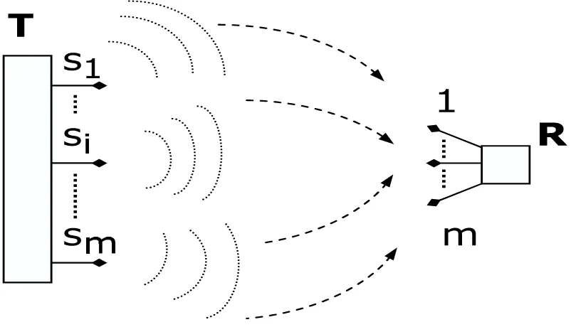
[image:14.612.89.490.401.631.2]

Although modern wireless devices provide great services, some of them (e.g., video-transmitting) that require high data rate transmissions are still unavailable. In last 10–15 years the idea of using multiple antennas instead of a single antenna at both the receiving and the transmitting ends of the point-to-point communication system (depicted in Figure 1.1), has become a subject of extensive theoretical and practical research. The main idea is that adding the antennas should increase the amount of information that can be transmitted. It in fact was mathematically shown in [95] and [40] that the achievable transmission rate increases linearly with the number of transmitting/receiveing antennas, provided that the transmission medium is Gaussian. These results are of course more on a theoretical side. It still remains an open question how to practically design these systems and achieve the theoretically predicted performances.

Figure 1.1: Multi-antenna system

(15)

to solving hard combinatorial optimization problems. A large portion of this thesis is related to improving the current detection techniques. Practically, this means that a large part of this thesis is focused on the design of the new and the improvement of the existing exact and approximate optimization algorithms for solving these hard problems.

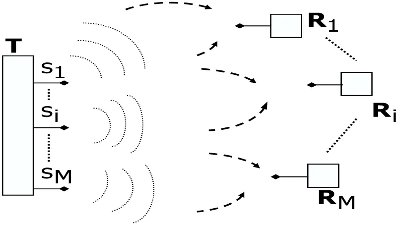
As we have said, the multiple antennas can be employed in the so-called point-to-point communication. Point-to-point communication assumes that there are two ends of com-munication, the transmitter and the receiver. Furthermore the assumption in the context of wireless communications is that they communicate through wireless medium. Another interesting concept of communicating that wireless medium allows is called broadcast com-munication. In broadcast communication one transmitter (say a base station) broadcasts the information that can be received by different users (see Figure 1.2). In the literature this system is often called a broadcast channel. Similar to point-to-point communication, in broadcast communication the transmitter and the receivers can be equipped with multiple antennas. The main idea is that if the transmitter is equipped with, say,mantennas, it can simultaneously serve m users. However, since the transmission medium is transparent for all signals, parts of the information intended for one of the users will reach users that are not intended to receive it. The piece of non-intended information which reaches receivers may cause them to incorrectly detect the information intended for them. This problem (commonly known as interference) is caused by the fading nature of the wireless broadcast medium and is one of the main issues in wireless broadcast systems. The problem of design-ing the information symbol vectors at the transmitter so that the problem of interference among the users is as mitigated as possible has been extensively studied during the last decade. Significant theoretical results related to the performance limits of broadcast chan-nels have been achieved. Surprisingly, the fading characteristics of the channel can in fact be utilized so that the expected increase in the overall amount of information that can be reliably transmitted is achieved.

(16)

[image:16.612.90.494.215.442.2]

in a point-to-point system, in a broadcast channel we define sum-rate capacity to be the maximum achievable sum of the rates of information that can be reliably sent to the users. In addition to this, we can define the achievable rate region as the set of the rates at which the information can be sent to the individual users. It is not difficult to note that the sum-rate capacity is the point on the boundary of the rate region that maximizes the sum of all individual rates.

Figure 1.2: Wireless broadcast system

As we have mentioned above, during the last decade the analysis of the performance limits of broadcast channels has been the subject of extensive research. Namely, the achiev-able sum-rate of the Gaussian broadcast channel has recently been computed [101], and a particular strategy called dirty-paper coding (DPC) introduced in [20] has been proven to achieve it (see, e.g., [14] and [112]). Furthermore, it also happens that the DPC achieves all points on the boundary of the rate region of the broadcast channel. However, DPC is a very complex technique and difficult to implement in practice. In this thesis we introduce a few alternatives to DPC and analyze their performance.

(17)

fact they all hold under the assumption that the transmitter has full knowledge of the transmission medium. In this thesis we will focus exactly on this same case when the characteristics of the broadcast channel don’t change rapidly in time so that they can be estimated. Furthermore, we will mostly focus on the case where the number of the users served by the transmitter (base station) is of similar order as the number of the transmitting antennas. On the other hand we would like to mention that, even when the transmitter has only a partial information about the channel and the number of the receivers/users is large, the sum-rate capacity asymptotically scales linearly in number of transmitting antennasm

and doubly logarithmic in the number of users — effectively the same way the sum-rate capacity of the optimal DPC scales with the number of transmitting antennas and the number of users (see, e.g., [83]).

1.1

Thesis contributions

This thesis contains three main parts. The first two deal with the problems related to the multiple-antenna point-to-point and broadcast channels. The third part is somewhat different and is related to the specific problem of quantum detection in quantum systems.

1.1.1 ML detection

In the first part of the thesis we consider multiple-input multiple-output (MIMO) systems. A point-to-point communication system which consists of one transmitter and one receiver equipped with multiple (m) antennas is an example of a MIMO system. As we have said above, one of the key problems in designing these systems is the complexity of the receiver. It is very well known that in MIMO systems maximum-likelihood (ML) detection of the received signals amounts to solving integer least-squares problems which are NP-hard in worst case. Since NP-hard problems may require a very long time to be solved exactly, it is of great interest to find efficient algorithms that can be practically implemented.

(18)

(trans-mission medium). This is a valid assumption if the communication occurs under non-rapidly changing environmental conditions so that the channel can be estimated. The problem of MIMO detection then becomes the integer least-squares problem (see, e.g., [49]). Usually in the context of wireless communications a specific algorithm called sphere-decoder (more on the sphere decoder can be found in [37]) is used for solving ML detection problems. Since the algorithm is used in a statistical system as a measure of its quality, a quantity called the expected complexity is usually considered in the literature (see, e.g., [49]). In fact, as shown in [49], the expected complexity over the wide range of the signal-to-noise (SNR) ratios and the dimension of the problem m is smaller than m3_{. However, when} the SNR decreases and the dimension of the problem grows, the complexity of the sphere decoder becomes prohibitive. In Chapter 2 we develop a branch and bound modification of the standard sphere decoder algorithm and demonstrate that it significantly decreases the size of the search tree compared to the original version of the algorithm. Furthermore, we establish an interesting mathematical connection between the H-infinity estimation theory and the lower bounding of the integer least-squares.

(19)

1.1.2 Broadcast channels

In the second part of the thesis (Chapters 4 and 5) we consider a Gaussian broadcast channel. In Chapter 4 we introduce a few practical schemes based on the linear precoding for the design of the information symbols at the transmitter in a Gaussian broadcast channel. We design the precoding strategy: 1) so that the overall sum-rate is maximized and 2) so that the minimum rate among all users is maximized. The later one is shown to be a quasi convex problem and solved exactly.

In Chapter 5 we analyze the theoretical limits of a particular non-linear scheme called vector-perturbation technique introduced in [75]. It turns out that an even simpler version of it, based on the nulling and cancelling procedure, asymptotically achieves the sum-rate of the DPC.

1.1.3 Quantum unambiguous detection

In the third part of the thesis (Chapters 6 and 7) we consider quantum systems. More specifically the problems that we are interested in are related to the quantum detection theory.

In quantum systems, unlike in classical, the information is stored in special objects called quantum states. Namely a quantum state is a set of numbers which fully describes the quantum system. These numbers are usually stored in a vector called a pure state [73]. Furthermore, the state of a quantum system can be a statistical mixture of pure states, in which case it is called a mixed quantum state [73].

(20)

We then consider state sets with strong symmetry properties, and show that the optimal measurement operators for distinguishing between these states share the same symmetries, and can be computed very efficiently by solving a reduced size semi-definite program.

(21)

Chapter 2

Coherent ML Detection in

Multi-Antenna Systems — Sphere

Decoder Algorithm

2.1

Introduction

(22)

[image:22.612.92.489.101.331.2]

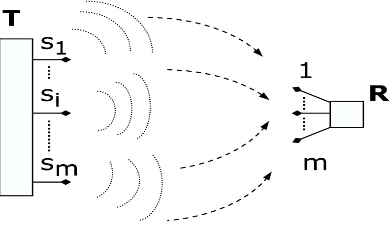
at the receiver in a MIMO system.

Figure 2.1: Multi-antenna system

Before going exactly to the specific problem, let us elaborate briefly on the the way a MIMO system works and how it is typically modeled. As can be seen from Figure 2.1, the system consists of the transmitterTand and receiverR, which both havemantennas. The transmitter then sends the sequence (vector) of the information symbols s, as depicted in Figure 2.1. The signals from the vector s are sent as electromagnetic waves through the transmission medium (air) such that signal si,1 ≤ i ≤ m is sent from the i-th antenna. Since the transmission medium is air, the signals sent from any ofm transmitter antennas can reach any of mreceiver antennas. It is usually assumed that the signals from different transmitting antennas are combined in a linear fashion at the receiver. This mathematical simplification of a real MIMO system is shown in Figure 2.2.

(23)

[image:23.612.119.529.57.314.2]

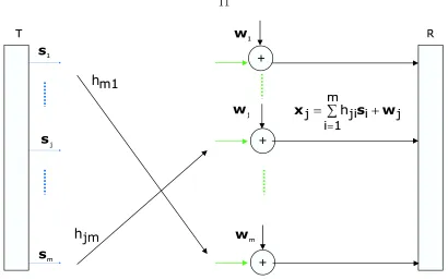
Figure 2.2: Mathematical model of multi-antenna system

entry of the matrixH will contain the characteristics of the path fromi-th transmitting to thej-th receiving antenna. In context of wireless communications the matrixH is usually called the channel matrix. Additionally, signal at the each of the receiving antennas is corrupted by noise (for the j-th receiving antenna this is shown in Figure 2.2 as quantity

wj). It is not difficult to see that the models from Figures 2.1 and 2.2 can be summarized in the following equation

x=Hs+w. (2.1)

As we have said earlier, H is the channel matrix and w is the noise vector. To allow tractability of the model it is usually assumed that the channel matrix coefficients are i.i.d. Gaussian random variables with zero mean and unit variance. The components of the noise vector w are also assumed to be i.i.d. Gaussian, independent of the entries of the channel matrixH, with zero mean and variance σ2.

(24)

of the vector x (its components are signals received at the receiving antennas, i.e., they are known to the receiver), can one somehow figure out what the value of the signal vector s was? In fact this is precisely the question of signal detection in multi-antenna systems. In the most general setting this question is very difficult. Not only don’t we know the matrix H, but knowledge of the vector w is also absent. Clearly, following this argument we recognize that learning H at the receiver is an important question. This has of course been the subject of extensive research, and in situations where the channel coefficients from the matrixH are not changing rapidly in time, they can in fact be estimated [47]. The case when the channel matrix is known at the receiver is usually referred to as the coherent case of the signal detection in multi-antenna systems. In the rest of this chapter we will assume communication in the slowly changing environment, so that the channel matrix is known to us. [We will elaborate more on the non-coherent case, when the channel matrix can not be estimated, in the following chapter.]

Looking at equation (2.1) we can write

p(x_|s, H) = _√1 2πne

−||x−Hs||22

2 . (2.2)

Then we can set the maximization of the probability from (2.2) as a criterion for the detection of the signal vector s if the received vector x and the channel matrix H are known. The detected vector sML is then

sML= arg min

s∈Dp(x|s, H) = arg mins∈D||x−Hs||

2

2. (2.3)

This criterion for signal detection in MIMO systems is called maximum-likelihood (ML) detection. It should also be noted that the vector sis restricted to a set_D, which in digital communications is commonly assumed to be a subset of the integer lattice.

(25)

range of dimensionsN and signal-to-noise ratios (SNRs), the sphere decoding algorithm [37] can be used to find the exact ML solution with an expected complexity that is often less thanN3. However, the computational complexity of sphere decoding becomes prohibitive if the signal-to-noise ratio (SNR) is too low and/or if the dimension of the problem m is too large.

In this chapter, we target these two regimes and attempt to find faster algorithms by pruning the search tree beyond what is done in the standard sphere decoding algorithm. The search tree is pruned by computing lower bounds on the optimal value of the objective function as the algorithm proceeds to descend down the search tree. We observe a trade-off between the computational complexity required to compute a lower bound and the size of the pruned tree: the more effort we spend in computing a tight lower bound, the more branches that can be eliminated in the tree. Using ideas from SDP-duality theory andH∞

estimation theory, we propose general frameworks for computing lower bounds on integer least-squares problems. We propose two families of algorithms, one of which is appropriate for large problem dimensions and binary modulation, and the other of which is appropriate for moderate-size dimensions yet high-order constellations. We then show how in each case these bounds can be efficiently incorporated in the sphere decoding algorithm, often resulting in significant improvement of the expected complexity of solving the ML decoding problem, while maintaining the exact ML performance.

2.2

Sphere decoder and its modification

In this section we recall what the standard sphere decoder is and introduce its branch and bound modification. We recall that the problem that we are interested in and will be solving

exactly in this chapter has the following form

min

(26)

where x ∈ Rn_, _H _{∈ R}n×m_{, and} _D _{refers to some subset of the integer lattice} _Zm_{. The} main idea of the sphere decoder algorithm [37] for solving the previous problem is based on finding all points s such that Hs lies within a sphere of some adequately chosen radius ds centered at x, i.e., on finding alls such that

d2_s_{≥ k}x₋Hs_k2₂, (2.5)

and then choosing the one that minimizes the objective function. Using theQR decompo-sitionH=

Q1 Q2

 

 R

0n−m×m

 

, whereRism×m upper triangular, andQ1∈Rn×m and

Q2 ∈Rn×(n−m) are such that Q=

Q1 Q2

is unitary, we can reformulate (2.5) as

d2_{≥ k}y₋Rs_k2₂, (2.6)

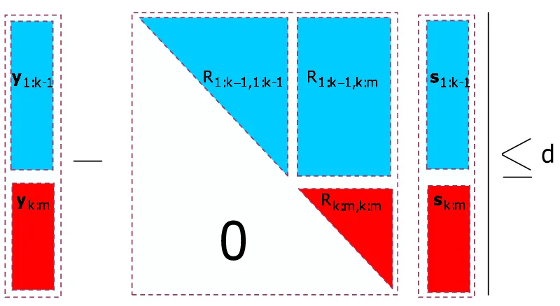
[image:26.612.95.495.414.633.2]

where we have definedd2 =d2_s− kQ∗₂y_k2 and y=Q∗₁x.

Figure 2.3: Upper-triangular decomposition — the key component of the sphere decoder algorithm

(27)

rewritten as

d2 _{≥ k}yk:m−Rk:m,k:msk:mk2+ky1:k−1−R1:k−1,1:k−1s1:k−1−R1:k−1,k:msk:mk2, (2.7)

for any 2 ≤ k ≤ m, where the subscripts determine the entries the various vectors and matrices run over (e.g., y1:k−1 is a column vector whose components are y1,y2, . . . ,yk−1, and similarlyR1:k−1,k:m is a (k−1)×(m−k+ 1) matrix andRi,k, Ri,k+1, . . . , Ri,m are the components of its i-th row). A necessary condition for (2.6) can therefore be obtained by omitting the second term on the right-hand side (RHS) of the above expression to yield

d2≥ ky_k_:_m₋Rk:m,k:msk:mk2. (2.8)

The sphere decoder finds all pointssin (2.5) by proceeding inductively on (2.8), starting from k = m and proceeding to k = 1. In other words, for k = m it determines all one-dimensional lattice points sm such that

d2 ≥(ym−Rm,msm)2,

and then, for each such one-dimensional lattice pointsm, determines all possible values for sm−1 such that

d2 _{≥ k}ym−1:m−Rm−1:m,m−1:msm−1:mk2

= (ym−Rm,msm)2+ (ym−1−Rm−1,m−1sm−1−Rm−1,msm)2.

(28)

[image:28.612.86.492.102.343.2]

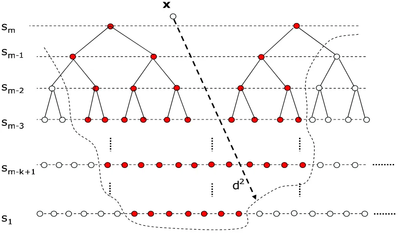
an explicit description of the algorithm the reader may refer to [37], [23], and [49].)

Figure 2.4: Tree generated by the sphere decoder algorithm

The computational complexity of the sphere decoding algorithm depends on how d is chosen. In a digital communication context, xis the received signal, i.e., a noisy version of the symbol vector s transmitted across the channel H,

x=Hs+w, (2.9)

where the entries of the additive noise vectorware independent, identically distributed (iid) N(0, σ2_{) random variables. In [49] it is shown that, if elements of} _H _{are i.i.d. Gaussian} with zero mean and unit variance and if the radius is chosen appropriately based on the statistical characteristics of the noise w, then over a wide range of signal-to-noise ratios (SNR) and problem dimensions the expected complexity of the sphere-decoding algorithm is low and comparable to the complexity of the best known heuristics, which are cubic.

(29)

is always exponential). Increasing the dimension of the problem clearly is useful 1. More-over, the use of the sphere decoder in low SNR situations is also important, especially when one is interested in obtaining soft information to pass onto an iterative decoder (see, e.g., [52] and [98]). One way to reduce the computational complexity is to resort to suboptimal methods based either on heuristics (see, e.g., [5]) or some form of statistical pruning (see [43]). Also, the interested reader may find more about recent improvements and alternative techniques in [22], [110], [45], [65], and [103].

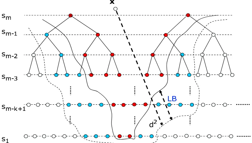
In this chapter, we attempt to reduce the computational complexity of the sphere de-coder while still finding the exact solution. Let us surmise on how this may be done. As mentioned above, the sphere decoding algorithm generates a tree whose number of branches at each level corresponds to the number of lattice points satisfying (2.8). Clearly, the com-plexity of the algorithm depends on the size of this tree, since each branch in the tree is visited and appropriate computations are then performed. Thus, one approach to decrease the complexity is to reduce the size of the tree beyond that which is suggested by (2.8). To this end, consider a lower bound on the optimal value of the second term on the RHS of (2.7):

LB=LB(y1:k−1, R1:k−1,1:m,sk:m)≤ min

s1:k−1∈D⊂Zk−1

ky1:k−1−R1:k−1,1:k−1s1:k−1−R1:k−1,k:msk:mk2,

where we have emphasized the fact that the lower bound is a function ofy_1:_k₋₁, R1:k−1,1:m, and sk:m. Provided our lower bound is nontrivial (i.e., LB >0), we can replace (2.8) by2

d2−LB≥ kyk:m−Rk:m,k:msk:mk2. (2.10)

This is certainly a more restrictive condition than (2.8), and so will lead to eliminating more points from the tree as illustrated in Figure (2.5). Note that (2.10) will not result in missing

1_{Various space-time codes result in integer least-squares problems where the problem dimension is much}

larger than the number of transmit antennas. Also, in distributed space-time codes for wireless relay networks the problem dimension is equal to the number of relay nodes, which can be quite large ([64] and [61]).

(30)

any lattice points from (2.5) since we have used alower boundfor the remainder of the cost in (2.7) (for more on branch and bounding ideas, the interested reader may refer to [70] and the references therein). Assuming that we have some way of computing a lower bound

[image:30.612.84.491.335.566.2]

LB > 0 as suggested above, we state the modification of the standard sphere decoding algorithm based on (2.10). The algorithm uses the Schnorr-Euchner (S-E) strategy with radius update [2]. [Note that in this chapter we consider several modifications of the sphere decoding algorithm, and all are implemented using Algorithm 1 below. The difference between the various modifications is how the value of LB in step 4 of the algorithm is computed. Also, note that in Algorithm 1, given below,_D is the full integer lattice, while later in this chapter, in different modifications of the original algorithm, it will be restricted to its subsets.]

Figure 2.5: Reduced tree of the branch and bound sphere decoding algorithm

Algorithm 1:

Input: Q, R, x, y=Q∗₁x, d= ˆd, ll1:m=01×m.

(31)

2. (Bounds for s_k) Set ub(s_k) = b

q

d2

k−(d2−dˆ2)+yk|k+1

rk,k c, lb(sk) = d

−qd2

k−(d2−dˆ2)+yk|k+1

rk,k e,

lk=blb(sk)+ub₂(sk)+1c, uk=lk+ 1. 3. (Zig-zag throughsk)

Ifllk= 0,sk=lk, lk=lk−1,llk= 1, otherwise sk =uk, uk =uk+ 1, llk = 0. Iflb(s_k)≤s_k_≤ub(s_k), go to 4, else go to 5.

4. If LB(y1:k−1, R1:k−1,1:m,sk:m) + (yk|k+1−rk,ksk)2−d2_k+ (d2−dˆ2)>0, go to 3, else go to 6.

5. (Increasek) k =k+ 1; ifk =m+ 1 terminate algorithm, else go to 3.

6. (Decrease k) If k = 1 go to 7. Else k = k ₋1, yk|k+1 = yk−Pmj=k+1rk,jsj, d2k =

d2

k+1−(yk+1|k+2−rk+1,k+1sk+1)2, and go to 2.

7. Solution found. Save s and its distance fromx, ˆd=d2

m−d21+ (y1−r1,1s1)2, and go to 3.

Clearly, the tighter the lower bound LB, the more points will be pruned from the tree. Of course, we cannot hope to find the optimal lower bound, since this requires solving an integer least-squares problem (which was our original problem to begin with). Therefore, in what follows we focus on obtaining computationally feasible lower bounds on the integer least-squares problem

min

s1:k−1∈D⊂Zk−1

kz1:k−1−R1:k−1,1:k−1s1:k−1k2, (2.11)

where, for simplicity, we introducedz(k−1) =z1:k−1 =y1:k−1−R1:k−1,k:msk:m. Also, in the rest of this chapter we will assume D={−M−1

2 ,−M2−3, . . . ,M2−3,M2−1}m, the case which is of interest in communications applications.

(32)

a lower bound. An even more basic question, perhaps, is what are the potential pruning capabilities of the lower bounding technique which we use to modify the sphere decoding algorithm. To illustrate this, consider a simple lower bound (which is only valid in the binary case, i.e., if D = {−12,12}m) on (2.11), used earlier in [88] and further considered in Section 2.3, which is based on duality and may be computed by solving the following semi-definite program (SDP),

max

Λ Tr(Λ)

subject to QΛ, Λ is diagonal, (2.12)

where

Q=

  

1

4RT1:k−1,1:k−1R1:k−1,1:k−1 −12RT1:k−1,1:k−1z1:k−1 −12zT1:k−1R1:k−1,1:k−1 zT1:k−1z1:k−1

  .

We mention that bounds of this type are very well known in the literature on semi-definite programming relaxations. More on them and their history can be found in [109]. Here we would like to only briefly mention the reason for their popularity. Although it is difficult to prove how tight these bounds are, it turns out that in practice they perform very well. On top of that, the optimization problem given above is convex (the objective function is convex and the region of optimization is convex as well) which means that these bounds can be computed very efficiently using a host of numerical methods [12]. Even more surprising, it can be proved that they can be computed in polynomial time.

(33)

and [1] the authors considered applications of SDP relaxation to problems in multiuser detection in CDMA systems. In [68], [63], [57], and [69] authors applied the SDP relaxation to the problem of ML-detection in MIMO systems (the same one that we consider in this chapter). In [69] the authors generalized the applications of the SDP algorithm from binary to larger constellations, and in [63] the authors proved that under certain conditions related to the dimension of the problem in high-SNR regime the SDP relaxation is tight.

As demonstrated in these references, the SDP technique can be very powerful in produc-ing a very good approximate solution of the original integer least squares problem. However in this work we focus on solving the integer least-squares problemexactly, and therefore we will only use its lower-bounding feature. It should also be noted that although in general suboptimal, the SDP technique can sometimes produce the exact solution to the original problem (for more on when this happens see [57]).

0 10 20 30 40 50 60 70 80

100 101 102 103 104 105 106 107 108

level

number of points per level

Distribution of points

[image:33.612.170.468.367.607.2]

SDPSD SD

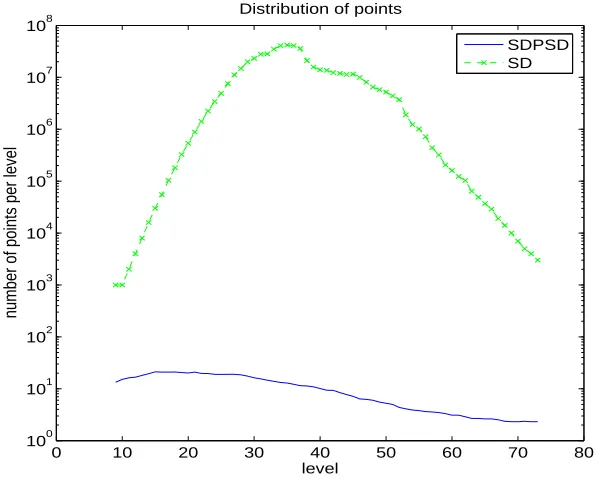
Figure 2.6: Comparison of the number of points per level in the search tree visited by the SD and the SDSDP algorithm, m= 100, SNR = 10 db,_D=_{−1₂,1₂_}m.

(34)

compares the number of points3 on each level of the search tree visited by the basic sphere decoding algorithm with the corresponding number of points visited by the modified sphere decoding algorithm which employsLBSDP for additional, lower-bound based, pruning. We refer to the former as the SD algorithm and to the latter as the SDSDP algorithm. As evident from Figure 2.6, for a problem of dimension m = 100, SNR= 10dB, and _D = {−1

2,12}m (i.e., BPSK modulation), the number of points in the search tree visited by the SDSDP algorithm is several orders of magnitude smaller than that visited by the SD algorithm. [The additional pruning of the search tree varies across the tree levels. The total number of the points visited by the SDSDP algorithm is roughly 106 _{times smaller} than that visited by the SD algorithm.] Therefore, a good lower bound can help prune the tree much more efficiently than the standard sphere decoding alone. However, computing

LBSDP requires solving an SDP per each point in the search tree. The computational effort of solving an SDP isO(k3.5_{), which is significantly greater than the linear complexity} of the operations performed by the standard sphere decoding algorithm at every visited node. Furthermore, although the complexity scaling behavior of solving an SDP is provably

O(N3.5), even for moderately large N (30 < N < 70) the real complexity of solving the SDP given in (2.12) is >> N3.5. On the other hand the standard sphere decoder performs per each node a number of operations that is _≈ N. Therefore, there is merit in searching not only for tight lower bounds such as the one in (2.12), but also for those that may not be as tight but which require significantly smaller computational effort.

In this chapter we therefore introduce a lower bound LBsdp on the quantity LBSDP which can be computed with complexity linear ink. The idea is based on efficient propaga-tion ofLBsdpthrough the search tree. We will show that the lower boundLBsdpsignificantly improves the expected complexity of the standard sphere decoder. However,LBSDP defined in (2.12) (and hence LBsdp) is a valid lower bound only when D={−1₂,1₂}m. To address the case of general _D, we derive another family of lower bounds on integer least-squares problems using ideas from H∞estimation theory. We show that several lower bounds that

(35)

may otherwise be obtained by relaxing the optimization constraints, are in fact special cases of our generalH∞-based lower bound. When employing the above lower bounds to modify sphere decoding, we observe a trade-off between the computational complexity required to compute a lower bound and the size of the pruned tree: the more effort we spend in com-puting a tight lower bound, the more branches can be eliminated from the tree. We show that the most computationally efficient among the special cases, the so-called eigenbound, provides a significant improvement in the expected complexity over the sphere decoding algorithm.

The rest of this chapter is organized as follows. In Section 2.3 we derive a compu-tationally efficient lower bound LBsdp on LBSDP. In Section 2.4, we derive the general

H∞-estimation-based lower bound on integer least-squares problem. In Sections 2.5, 2.6, and 2.8, special cases of this general bound are considered. In particular, the so-called spher-ical relaxation bound is derived in Section 2.5, the polytope relaxation bound is considered in Section 2.6, and the eigen bound is studied in Section 2.8. The effects of the aforemen-tioned bounds on the number of search tree points and/or the total expected complexity of the modified sphere decoding algorithm are studied throughout. Some simulations are presented in Section 2.7, and, finally, Section 2.9 contains conclusions and a discussion of potential extensions of the current work.

2.3

SDP-based lower bound

LetLB_SDP(k−1),1≤k≤m denote the optimal value of the following optimization problem,

LB_SDP(k−1) = max Tr(Λ)

subject to Qk−1 Λ, Λ is diagonal, (2.13)

where

Qk−1=

  

1

4RT1:k−1,1:k−1R1:k−1,1:k−1 −12RT1:k−1,1:k−1z(k−1) −12(z(k−1))TR1:k−1,1:k−1 (z(k−1))Tz(k−1)

(36)

In this section we deriveLB_sdp(k−1), a lower bound on LB_SDP(k−1). To this end, let ˆΛ denote the optimal solution of

max Tr(Λ)

subject to QΛ, Λ is diagonal, (2.14)

where

Q=

  

1

4RTR −12RTy −1

2yTR yTy

  .

LetGGT = 1₄RTR−Λˆ1:m,1:m, whereGis a lower triangular matrix. Also, letM =G−1RT. Using the fact that the matricesG andRT _{are lower triangular, we obtain}

(G1:k−1,1:k−1)−1 = (G−1)1:k−1,1:k−1,

G1:k−1,1:k−1(G1:k−1,1:k−1)T = 1 4R

T

1:k−1,1:k−1R1:k−1,1:k−1−Λˆ1:k−1,1:k−1,

and M1:k−1,1:k−1 = (G1:k−1,1:k−1)−1RT_1:_k₋₁_,_1:_k₋₁. Furthermore, let

λk= (z(k−1))Tz(k−1)− 1 4(z

(k−1)₎T_MT

1:k−1,1:k−1M1:k−1,1:k−1z(k−1), (2.15)

and let

LB_sdp(k−1)=

      

Pk−1

i=1 Λî,i+λk if Pik=1−1Λî,i+λk ≥0 0 if Pk_i₌₁−1Λî,i+λk <0.

(2.16)

Now it is clear thatLB_sdp(k−1)≤LB_SDP(k−1) since

LB_sdp(k−1) = Tr(diag( ˆΛ1,1,Λˆ2,2, . . . ,Λˆk−1,k−1, λk)),

(37)

We refer to Algorithm 1 which, in step 4, makes use ofLB(_sdpk−1) as the SDsdp algorithm. The subroutine for computing LB(_sdpk−1) is given below. Clearly, using LB_sdp(k−1) instead of

LB(_SDPk−1) results in pruning fewer points in the search tree. However, the computation of

LB(_sdpk−1) is quite a bit more efficient than the cubic computation ofLB_SDP(k−1). In particular, unlike in the SDSDP algorithm, we need to solve only one SDP — the one given by (2.14). Then we may computeLB_sdp(k−2) recursively fromLB_sdp(k−1), which requires complexity linear ink [92]. This is shown next.

Recall that z(k−1) = y1:k−1 −R1:k−1,k:msk:m. It is easy to see that we can compute z(k−2) fromz(k−1) as

z(k−2)=z(_1:k_k−₋1)₂₋R1:k−2,k−1sk−1. (2.17)

Furthermore, note that p(k−1)=M1:k−1,1:k−1z(k−1) can be computed recursively as

p(k−2) = M1:k−2,1:k−2z(k−2)

= M1:k−2,1:k−2(z_1:(k_k−₋1)₂−R1:k−2,k−1sk−1)

= M1:k−2,1:k−2(z(k−1))1:k−2−M1:k−2,1:k−2R1:k−2,k−1sk−1

= p(_1:k_k−₋1)₂₋(M R)1:k−2,k−1sk−1. (2.18)

Using p(k−2) and z(k−2) we computeλk−1 from (2.15), and LB_sdp(k−2) from (2.16). The computation ofLB_sdp(k−2) in each node at the (m−(k−2))th level of the search tree requires 4(k₋2) additions and 2(k₋2) multiplications. For the basic sphere decoder, the number of operations per each node at the (m−k+ 1)th level is (2k+ 17). This essentially means that the SDsdp algorithm performs about four times more operations per each node of the tree than the standard sphere decoder algorithm. In other words, if the SDsdp algorithm prunes at least four times more points than the basic sphere decoder, the new algorithm is faster in terms of the flop count.

Subroutine for computing LBsdp:

(38)

1. Ifk =m, solve (2.14) and set ˆΛ to be the optimal solution of (2.14);λk= (z(k−1))Tz(k−1)− 1

4(z(k−1))TM1:Tk−1,1:k−1M1:k−1,1:k−1z(k−1). 2. If 1< k < m,

2.1 z(k−1) =z_1:(k_k)₋₁₋R1:k−1,ksk, p(k−1) =p(_1:k_k)₋₁−(M R)1:k−1,ksk. 2.2 λk = (z(k−1))Tz(k−1)−1₄(p(k−1))Tp(k−1).

3 If λk≥0,LBsdp(k−1)=

Pk−1

i=1 Λˆi,i+λk, otherwise LBsdp= 0.

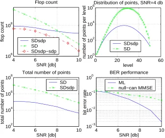
Figure 2.7 compares the expected complexity of the SDsdp algorithm to the expected complexity of the standard sphere decoder algorithm (SD-algorithm). The two algorithms are employed for solving a high-dimensional binary integer least-squares problem. The signal-to-noise ratio in Figure 2.7 is defined as SNR = 10log₁₀₄m_σ2, whereσ2 is the variance

of each component of the noise vector w. Both algorithms choose an initial search radius statistically as in [49] (the sequence ofs,= 0.9,= 0.99, = 0.999 etc.), and update the radius every time the bottom of the tree is reached.

As can be seen from Figure 2.7 the SDsdp algorithm can run up to 10 times faster than the SD algorithm at SNR 4₋5 db. At higher SNR, the speedup decreases and at SNR 8 db the SD algorithm is faster. We can attribute this to the complexity of performing the original SDP (2.14). In fact, Figure 2.7, subplot 1, shows the flop count of the SD-sdp, when the computations of the SDP (2.14) are removed (denoted there as SDsdp-sdp), which can be seen to be uniformly faster than the SD. Thus, the main bottleneck is solving (2.14) and any computational improvement there can have a significant impact on our algorithm. In our numerical experiments we solved (2.14) exactly, i.e., with very high numerical precision which requires a significant computational effort. This is of course not necessary. In fact how precisely (2.14) needs to be solved is a very interesting question. For this reason we emphasize again that constructing faster SDP algorithms would significantly speed up the SDsdp algorithm.

(39)

the size of the tree may be as important as the overall number of multiplication and addition operations. On subplot 3 of Figure 2.7 the comparison of the total number of points kept in the tree by SD and SDsdp algorithms is shown. As expected the SDsdp algorithm keeps significantly less points in the tree than the SD algorithm.

Finally on subplot 4 of Figure 2.7, the comparison of the bit error rate (BER) perfor-mance of the exact ML detector (SDsdp algorithm) and the approximate MMSE nulling and cancelling with optimal ordering heuristic is shown. Over the range of SNRs considered here, the ML detector outperforms the MMSE detector significantly, thereby justifying our efforts in constructing more efficient ML algorithms.

Remark: Recall that the lower bound introduced in this section is valid only if the origi-nal problem is binary, i.e.,D={−1

2,12}k−1. A generalization to caseD={−32,−12, 12,32}k−1 can be found in [106]. It is not difficult to generalize it to any_D=_{−L−₂1,₋L−₂2, . . . ,L−₂3,L−₂1_}k−1 by noting that any k −1-dimensional vector whose elements are numbers from {−L+ 1,₋L+ 2, . . . , L₋2, L₋1_}can be represented as a linear transformation of a (k₋1)(L₋ 1)-dimensional vector from D = {−1

2,12}(k−1)(L−1). (The interested reader can find more on this in [69]). However, this significantly increases the dimension of the SDP problem in (2.14), which may cause our algorithm to be inefficient. Motivated by this, in the following section we consider a different framework, based onH∞ estimation theory, which will (as we will see in Section 2.8) produce as a special case a general lower bound applicable for any D.

2.4

H

∞

-based lower bound

(40)

4 6 8 10 106 108 SNR [db] flop count Flop count SDsdp SD SDsdp−sdp

0 20 40 60

100

102

104

106

level

number of points per level

Distribution of points, SNR=4 db

SDsdp SD

4 6 8 10

102

104

106

108

SNR [db]

total number of points

Total number of points

SD SDsdp

4 6 8 10

10−3

10−2

10−1

100

SNR [db]

bit error rate

BER performance

[image:40.612.120.457.77.358.2]

ML null−can MMSE

Figure 2.7: Computational complexity of the SD and SDsdp algorithms, m = 50, _D = {−12,12}50

To simplify the notation, we rewrite (2.11) as

min

a∈D⊂Zk−1kb−Lak

2_, _(2.19)

where we introduceda=s1:k−1,b=z1:k−1, and L=R1:k−1,1:k−1.

Consider an estimation problem where a and b₋La are unknown vectors, b is the observation, and the quantities we want to estimate are a and b. In the H∞ framework, the goal is to construct estimators ˆa =f1(b) and ˆb =f2(b), such that for some given γ, some β ≥0, and some diagonal matrixD >0, we have

β_||a₋aˆ_||2+_||b₋bˆ_||2 a∗_D_a₊_k_b₋_L_a_k2 ≤γ

2 _(2.20)

forall a andb (see, e.g., [48]).

(41)

a andb we can write

kb₋La_k2 _≥γ−2β_||a₋ˆa_||2+_||b₋bˆ_||2₋a∗Da, (2.21)

and, in particular,

min

a∈Dkb−Lak

2 _≥_min

a∈D γ

−2_β_||_a₋_a_ˆ_||2₋_a∗_D_a₊_γ−2_||_b₋_b_ˆ_||2_. _(2.22)

Note that the minimization on the right-hand side (RHS) of (2.22) is straightforward since it can be done componentwise (which is why we chose D > 0 diagonal). Thus, for any H∞ estimators â =f1(b) and ˆb =f2(b), (2.22) provides a readily computable lower bound. The issue, of course, is how to obtain the best âand ˆb (andD and γ). To this end, let us assume that the estimators are linear, i.e., â=K1b and ˆb=K2b for some matrices

K1 and K2 (see Figure 2.8).

- - ? -a L

b₋La

K1 K2 ˆ a ˆ b

Figure 2.8: An H∞ estimation analogy used in deriving a lower bound on integer least-squares problem.

Introducing c=

  D

1/2_a

b₋La

 

and noting that

T =

  D

−1/2 ₀

LD−1/2 I   −

  K1

K2

  

LD−1/2 I =    √

β(I₋K1L)D−1/2 −√βK1 (I₋K2)LD−1/2 I−K2

(42)

maps c to

  

√

β(a₋ˆa) b₋bˆ

 

, from (2.21) we see that for all cit must hold that

c∗T∗Tc_≤γ2c∗Ic

(see [48]). SinceT is square, this implies either of the equivalent inequalities

T T∗ _≤γ2I or T∗T _≤γ2I. (2.23)

The tighter the bound in (2.23), the tighter the bound in (2.22). In other words, the closer

γ−1T is to a unitary matrix, the tighter (2.22) becomes. Hence we attempt to choose K1 and K2 to make γ−2T T∗ as close to identity as possible.

To this end, post multiply T with the unitary matrix

Φ =

 

 ∇

−1 _D−1/2_L∗_∆−∗

−LD−1/2_∇−1 _∆−∗   .

∇and ∆ are found via the factorizations

D−1/2L∗LD−1/2+I =_∇∗_∇ and LD−1L∗+I = ∆∆∗, (2.24)

to obtain

TΦ =

 

A B

0 C  

 (2.25)

where

A=pβD−1/2_∇−1, B=pβ(D−1L∗∆−∗₋K1∆), and C= (I−K2)∆. (2.26)

ThusT T∗ _≤γ2_I _implies

  AA

∗₊_BB∗ _BC∗

CB∗ CC∗

 

(43)

Note that we have many degrees of freedom when choosing K1 and K2, and wish to make judicious choices. So, to simplify things, let us choose K2 such that CC∗ = γ12I for some 0_≤γ1≤γ. (Clearly, this can always be done, since from (2.24) we have that ∆ is invertible, and the simple choice K2 = I −γ1∆−1 will do the job.) To make half the eigenvalues of

γ−2_{T T}∗ _{unity, we set the Schur complement of the (2}_,_{2) entry of (2.27) to zero, i.e.,}

AA∗+BB∗−γ2I−BC∗(CC∗−γ2I)−1CB∗= 0. (2.28)

Using CC∗=C∗C=γ₁2I, it easily follows that

BB∗= (1− γ 2 1

γ2)(γ

2_I₋_AA∗₎_. _(2.29)

Using the definitions of Aand B from (2.26), we obtain

p βK1 =

p

βD−1L∗(LD−1L∗+I)−1−B∆−1. (2.30)

From the (1,1) entry of (2.27) it follows that

γ2I−(AA∗+BB∗)≥0,

which is the only constraint on γ. Combining this constraint with the definition of A from (2.26), the definition of ∇ from (2.24), and the expression forBB∗ from (2.29), we obtain that

γ2 ≥ β

λmin(D+L∗L)

.

We summarize the results of this section in the following theorem:

Theorem 2.1. Consider the integer least-squares problem (2.19). Then for any γ2 ≥ β

λmin(D+L∗L),0≤γ1 ≤γ, and any matricesD ≥0,B, and∆satisfying∆∆

(44)

and BB∗= (1₋γ12

γ2)(γ2I−β(D+L∗L)−1),

min

a∈Dkb−Lak

2 _≥_min

a∈Dγ

−2_||p_β_a₋p_βD−1_L∗₍_LD−1_L∗₊_I₎−1_b₊_B_∆−1_b_||2₋_a∗_D_a₊γ12

γ2||∆− 1_b_||2_.

Proof. Follows from the previous discussion, noting that

||b−bˆ||2 =||(I −K2)b||2 =||C∆−1b||2 =γ21||∆−1b||2

and

AA∗ =β(D+L∗L)−1.

The next corollary directly follows from Theorem 2.1.

Corollary 2.1. Consider the setting of the Theorem 1 and let β= 1. Then

min

a∈Dkb−Lak

2 _≥ _min

a∈Dγ

−2_||_a₋_D−1_L∗₍_LD−1_L∗ ₊_I₎−1_b₊_Bφ_||2₋_a∗_D_a₊ γ12

γ2||φ|| 2_,

(2.31)

where B is the unique symmetric square root of(1−γ12

γ2)(γ2I−(D+L∗L)−1), and φisany vector of the squared length b∗(I+LD−1L∗)−1b.

(45)

maximize the first term, we need to take γ as its smallest possible value, i.e., we set

γ2 = 1

λmin(D+L∗L)

.

This leads to the following result:

Corollary 2.2. Consider the setting of the Theorem 2.1 and letβ = 1. Then

min

a∈Dkb−Lak

2 _≥_λ

min(L∗L+D)||a−(L∗L+D)−1L∗b||2−a∗Da+b∗(I−L((L∗L+D)−1)L∗)b (2.32)

Remark: We would like to note that the bound given in the previous Corollary could have been also obtained in a faster way. Below we show a possible derivation that an anonymous reviewer has provided to us.

Let D be a diagonal matrix such that D≥0. Then we have

||b₋La_||2 =a∗L∗La₋2b∗La+b∗b=a∗(L∗L+D)a₋2b∗La+b∗b₋a∗Da

= (a−(L∗L+D)−1L∗b)∗(L∗L+D)(a−(L∗L+D)−1L∗b)−b∗L((L∗L+D)−1)L∗b+b∗b−a∗Da ≥λmin(L∗L+D)||a−(L∗L+D)−1L∗b||2−a∗Da+b∗(I−L((L∗L+D)−1)L∗)b

It is not difficult to see that this is precisely the same bound as the bound given in Corollary 2.2. The interested reader can find more on this type of bound in [96] and [79].

(46)

the search space is now relaxed from integers to a polytope, can also be deduced as a special case of the lower bound from Theorem 2.1. Finally, in Section 2.8, we use (2.32) to deduce the lower bound based on the minimum eigenvalue ofL∗L.

2.5

Spherical relaxation

Assume the setting of Theorem 2.1. Letγ1 →γ,β→0,D = _α1I, and ∆sph∆∗sph=αLL∗+I. Then

LB_sph(1) =_||∆−_sph1b_||2₋k−1

4α , (2.33)

is a special case of the general bound given in Theorem 2.1 and, therefore, a lower bound on the integer least-squares problem (2.11). Additionally, since being a special case, it is less tight than the general bound given in Theorem 2.1. Clearly, to makeLB_sph(1) as tight as possible, we should maximize (2.33) overα.

Consider the singular value decomposition (SVD) ofL, L=UΣVT_{, where}_U _and_V _are unitary matrices, and where Σ is diagonal matrix. Let σi be the i-th component on the main diagonal of Σ and letr be the rank of L. Also, let q1:k−1 =UTz1:k−1. Then we can write

LB_sph(1) = r

X

i=1

α−1_q2 i

σ2 i +α−1

−α−1k−1

4 . (2.34)

To maximize over α we differentiate to obtain

dLB_sph(1) d(α−1₎ =

r

X

i=1

( σiqi

σ2 i +α−1

)2−k−1

4 . (2.35)

Let ˆα denote the value of α which maximizesLB_sph(1). Then it easily follows that r

X

i=1

( σiqi

σ2 i + ˆα−1

)2 = k−1

4 . (2.36)

Note that if Pk_i₌₁−1(qi

σi)

2₋ k−1

(47)

(2.11) as

ˆ

LB_sph(1) =_k∆ˆ_sph−1b_k2₋k−1

4ˆα , (2.37)

where ˆ∆sph is any matrix such that ˆ∆sph∆ˆ∗sph= ˆαLL∗+I= ˆαR1:k−1,1:k−1R1:k−1,1:k−1∗+I, b = z1:k−1, and ˆα−1 is the unique solution of (2.36) if Pki=1−1(qσii)

2 ₋ k−1

4 > 0, and zero otherwise.

To obtain an interpretation of the bound we have derived, let us consider a bound obtained by a simple spherical relaxation. To this end, let us denote ˆLB(2)_sph = _kz1:k−1−

R1:k−1,1:k−1ˆs1:k−1k22, where ˆs1:k−1 is the solution of the following optimization problem,

min

s1:k−1 k

z1:k−1−R1:k−1,1:k−1s1:k−1k22

subject to

k−1

X

i=1

s2_i _≤ k−1

4 . (2.38)

This is a lower bound since the integer constraints have been relaxed to a spherical constraint that includes_{−1₂,1₂_}k_{. The solution of (2.38) can be found via Lagrange multipliers (see.} e.g., [42]), and it turns out that the optimal value of its objective function coincides with (2.37). Therefore, we conclude that

ˆ

LB(2)_sph= ˆLB(1)_sph,

and the lower bound obtained via spherical relaxation is indeed a special case of the general lower bound given in Theorem 2.1.

(48)

that the bound given in (2.38) is valid for the binary case. It can, however, be used for

M > 2 if the constraint in (2.38) is replaced by Pk_i₌₁−1s_i2 _≤ (M ₋1)2k−1

4 . However we believe that this type of bound is more useful in the binary case.

Now, let us unify the notation and write LBsph= ˆLB (1)

sph= ˆLB (2)

sph. We employ LBsph to modify the sphere decoding algorithm by substituting it in place of the lower bound in step 4 of Algorithm 1. The subroutine for computing LBsph is given below.

Subroutine for computing LBsph:

Input: y_1:_k₋₁, R1:k−1,k:m,sk:m, R1:k−1,1:k−1.

1. z1:k−1 =y1:k−1−R1:k−1,k:msk:m.

2. Compute the SVD of R1:k−1,1:k−1, R1:k−1,1:k−1=UΣVT, V = [v1, ...,vk−1].

3. Set q1:k−1=UTz1:k−1 and r= rank(R1:k−1,1:k−1).

4. If Pr_i₌₁(qi

σi)

2 _> k−1

4 , find λ∗ such that

Pr i=1( σi

qi

σ2 i+λ∗)

2 ₌ k−1

4 , and compute ˆs1:k−1 =

Pr

i=1(σσ2iqi i+λ∗

)vi and LBsph=Pri=1( λ

∗_q

i

σ2 i+λ∗

)vi.

5. IfPr_i₌₁(qi

σi)

2_≤ k−1

4 , set ˆs1:k−1 =

Pr

i=1(qσii)vi andLBsph= 0.

The computational complexity of finding the spherical lower bound by the above sub-routine is quadratic in k, and the bound needs to be computed at each point visited by Algorithm 1. That the complexity is only quadratic may not immediately seem obvious since we do need to compute the SVD of the matrixR1:k−1,1:k−1. Fortunately, however, this operation has to be performed only once for each level of the search tree, and hence can be done in advance (i.e., before Algorithm 1 even starts). Computing the SVD of matrices

R1:k−1,1:k−1,2≤k≤m, would require performing factorizations that are cubic ink for any 2≤k ≤m. However, using the results from [62] and [46], it can be shown that allm SVDs can, in fact, be computed with complexity that is cubic inm.

(49)

the SVD, these remaining operations do need to be performed per each point visited by the algorithm. In particular, computing the vector q requires finding UT_z

1:k−1, which is quadratic in k. Now, the matrix UT is constant at each level of the search tree, but the vectorz_1:_k₋₁differs from node to node. Clearly, this is the most significant part of the cost, and the computational complexity of findingLBsph is indeed quadratic.

2.5.1 Generalized spherical relaxation

In this subsection, we propose a generalization of the spherical lower bound. This general-ization is given by

LBgsph =

      

LBsph+DLB, if k∆ˆ−_sph1bk2−k_{4 ˆ}−_α1 >0,

0, otherwise,

(2.39)

where, as in (2.37),

LBsph=k∆ˆ−_sph1bk2−

k−1 4ˆα ,

ˆ

∆sph∆ˆ∗sph = ˆαLL∗+I, L = R1:k−1,1:k−1, b = z1:k−1, q = UTb, L = UΣVT, ˆα−1 is the unique solution of (2.36) if Pk_i₌₁−1(qi

σi)

2₋k−1

4 >0, and 0 otherwise, and where

DLB= min

a∈D(

1 ˆ

α +λmin(L

∗_L₎₎_k_a₋_αL_ˆ ∗_(ˆ_αLL∗₊_I₎−1_b_k2_. _(2.40)

Clearly, (2.39) is obtained from (2.32) by settingD= _α1_ˆIand is, therefore, a lower bound on the integer least-squares problem (2.11). Also, since LBgsph ≥ LBsph, the generalized spherical bound is tighter than the spherical bound. It is interesting to mention thatLBgsph was also obtained in [96] based on a different approach.

We refer to Algorithm 1 with LB = LBgsph as the GSPHSD algorithm. Since the generalized spherical bound is at least as tight as the spherical bound, we expect that the GSPSD algorithm prunes more points from the search tree than the SPHSD algorithm.

(50)

Subroutine for computing LBgsph:

Input: y1:k−1, R1:k−1,k:m,sk:m, R1:k−1,1:k−1

1. z1:k−1 =y1:k−1−R1:k−1,k:msk:m.

2. Compute the SVD of R1:k−1,1:k−1, R1:k−1,1:k−1=UΣVT, V = [v1, ...,vk−1]. 3. Set q_1:_k₋₁=UTz_1:_k₋₁ and r= rank(R1:k−1,1:k−1).

4. If Pr_i₌₁(qi

σi)

2 _> k−1

4 , find λ∗ such that

Pr

i=1(σσ2iqi i+λ∗)

2 ₌ k−1

4 , and compute ˆs1:k−1 =

Pr i=1( σi

qi

σ2 i+λ∗)

viandLBgsph= mina∈D(λ∗+λmin(R∗_1:_k₋₁_,_1:_k₋₁R1:k−1,1:k−1))ka−Pr1 σi

qi

σ2 i+λ∗

vik2+

Pr i=1( λ

∗_q

i

σ2 i+λ∗

)vi. 5. IfPr_i₌₁(qi

σi)

2_≤ k−1

4 , set ˆs1:k−1 =

Pr i=1(

qi

σi)vi andLBgsph= 0.

At first, the complexity of computing DLB in (2.40) may seem cubic in k; however, it can actually be reduced to quadratic. Clearly, finding the inverse of ˆαLL∗₊_I _{is of cubic}

complexity and required in each node of the search tree (Lis constant per level but ˆαdiffers from node to node). However, instead of inverting the matrix ˆαLL∗+I directly, we can do it in several steps. In particular, using the SVD L=UΣVT_{, we can write}

ˆ

αL∗(ˆαLL∗+I)−1b= ˆαVΣ(ˆαΣ2+I)−1Ub.

(51)

2.6

Polytope relaxation

In this subsection, we show that the lower bound on the integer least-squares problem (2.11) obtained by solving the related convex optimization where the search space is relaxed from integers to a polytope is yet another special case of the lower bound derived in Section 2.4. Assume the setting of the Theorem 2.1. Letγ1 →γ,β →0, and ∆plt∆∗plt =LD−1L∗+I. Then

LB(1)_plt =||∆−_plt1b||2₋TrD

4 (2.41)

is a special case of the general bound given in Theorem 2.1 and, therefore, a lower bound on the integer least-squares problem (2.11). Now, since the matrix D is a free parameter, we can make the bound (2.41) tighter by optimizing over D. Hence, we can obtain a lower bound to the integer least-squares problem (2.11) as

ˆ

LB(1)_plt = max D≥0||∆

−1 pltb||2−

TrD

4 . (2.42)

Clearly, ˆLB(1)_plt is also a lower bound on the integer least-squares problem (2.11). Further-more, since (2.42) allows for any positive semi-definite diagonal matrix D, while (2.33) allows only for scaled version of identity, it is clear that the bound in (2.42) will be tighter than the one in (2.33). However, as we will see in the rest of this section, computing (2.42) is of greater complexity than computing (2.33).

Now, before further discussing and comparing the merits of the bounds defined in (2.33) and (2.42), we will show that the lower bound (2.42) is equivalent to the lower bound obtained by relaxing the search space in the integer least-squares problem (2.11) to a poly-tope and solving the resulting convex optimization problem. In particular, such a relaxation yields

min _||b₋Ld_||2 subject to ₋1

2 ≤di ≤ 1

(52)

Let us denote ˆLB(2)_plt =_||b₋Ldˆ_||2, where ˆd is a solution of (2.43). We want to show that ˆ

LB(1)_plt = ˆLB(2)_plt. To this end, consider the Lagrange dual of the problem (2.43),

L(ξ) = ||b−Ld||2+ k−1

X

i=1

ξi(d2i − 1 4)

= d∗(L∗L+ Ξ)d₋2b∗Ld+b∗b₋TrΞ 4 = d∗ΩΩ∗d₋2b∗LΩ−∗Ω∗d+b∗b₋TrΞ

4 +b

∗_L_Ω−∗_Ω−1_L∗_b₋_b∗_L_Ω−∗_Ω−1_L∗_b