Radar methods for the exploration of glaciers

RADAR METHODS

FOR TEE EXPLORATION OF GLACIERS

Thesis by

Bernard Owen Steenson

In

Partial Fulfillment of the Requirements for the Degree of

Doctor of Philosophy

California Institute of Technology Pasadena~ California

ACKNOWLEDGMENTS

The author takea this opportunity to thank Professor

w

.

H. Pickering, who suggested this project and under whose guidance the work was conducted. He also expresses his gratitude to Professor R. P. Sharp, under whose excellent leadership the field work was

carried out, and who was consulted many times on problems of glaciology.

Mr

.

Fred Gross deserves appreciation for his able assistance during the entire 1949 phase of the work. The author also says thanks to 1~. Walter Wood and the other meJllbers of "Project Snow Cornice," with whom

it was a pleasure to work.

ABSTRACT

The problem of finding the depths of glaciers and the current methods are discussed briefly. Radar methods are suggested as a

pos-sible improvement for, or adjunct to, seismic and gravity survey methods. The feasibility of propagating electromagnetic waves in ice and the

maximum range to be expected are then investigated theoretically with the aid of experimental data on the dielectric properties of ice. It is found that the maximum expected range is great enough to measure the depth of many glaciers at the lower radar frequencies if there is not too much liquid water present. Greater ranges can be attained by going to lower frequencies.

PART

I I I III IV

v

VI

VII

VIII

INTRODUCTION.

TABLE OF CONTENTS

TITLE

.

.

.

.

.

. . .

.

.

. .

.

THEORY • • • •

.

. .

. .

.

. . .

.

.

.

. .

.

PRELIMINARY CONSIDERATIONS IN THE SELECTION OF

EQUIPMENT

• • • • • • • • • • • • • • • • • • •

. . .

.

1948

EXPEDITION

(a) Location and Equipment. • • • • •

(b) Operation and Results • • • • • • • • • • • • • ( o) Other Methods • • • • • • • • • • • • • • •

GLACIOLOGY. • •

•

• • • • • •

. .

.

.

1949

EXPEDITION

(a) Equipment • • • • • • • • • • • • • • • • • (b) Operation and Results • • • • • • •

(o) Other Methods • • • • • • • • • • • • • • •

ANALYSIS

OF

E

Q

UIPMENT

• • • • •

.

.

.

.

.

.

DISCUSSION.

REFERENCES. •

R.AD1AR

METHODS

FOR THE EXPLORATION OF GLACIERS

I. INTRODUCTION

The problem of finding the depths of glaciers comes under the subject of geophysics. The answers are of interest chiefly to geolo-gists~ but their determination involves the methods of the physicist. Sounding by seismic methods has been u~ed successfully on glaciers where the dynamite charges could be placed in the solid ice.(l) More

difficulty is experienced when the surface of the glacier·consists of a thick layer of nev~ or firn. This acts as a sort of cushion which absorbs the energy of the blast. Seiamic equipment is usually heavy enough so that considerable work is involved in transporting it; more -over~ it takes an appreciable amount of time to make a sounding~ especially if the surface layer of neve must be penetrated to place the charge in solid ice.

Gravity surveys can be used to give the configuration of the rock floor~ but not the depth. The depth at one or more control points can then be ascertained by other methods. Since the neighboring topog-raphy introduces corrections to the raw data, gravity surveys are best suited to regions where the surfaces of the glaciers and surrounding land are gentle. This method is still in the development stage for applQcation to glaciers, but undoubtedly will undergo more tests in the future, and probably will become an adjunct to other methods~ principally

seismic.

2

-II. THEORY

The solution of Maxwell's equations gives the formulas governing

the propagation of a plane wave in an imperfect dieleotric.(2) The

steady-state solution is

(2 .01)

where propagation is taken in the z direction and

y

:= ()( -t-

if

is the propagation constant. It is given by*

"' l. .,

y

:. _

t.u

/«-

£

+

/w /-'

tr

=

-t-v?

f. _(2.02}

where~ is the permeability and

{_,. f. (,

+

r)

=

£.(£'-,

d

(2.03)

is the complex permittivity. The conductivity is denoted by .- and

the permittivity of free space by

Eo.

The ratio of loss current to

charging current is given by

£1£'.

The loss angle

~

is defined by

,

~

( =

£

:::=

.sr:.-

(2.04)

4 £' w£

Solving for the real and imaginary parts of the propagation constant gives

The wave length is given by

_,)

A:;:

ET

(f

The wave impedance is given by

i

=

ff

naper s

I

meter

radians

I

meter

meters

ohms

For low loss materials where tan ~((l, these expressions become

*

The rationalized MKS system of units will be used.

(2.05)

(2. 06)

(2.07)

3

-0(=1_'1/£

~b

=

{).a,,

f

lto(

~~/

£1

;1a::n.. '

rJ~w'(ft£

.A=~

yu'c'

nepers

I

meter

db

I

meter (2. 09)

radians / meter (2.10)

meters (2.11)

where fmc is the frequency in megacycles per second, Ao is the free

space wavelength and

is the free space permeability. Also

f[

==

«

ohms (2.12)

Since the impedance of free space is 377 ohms, this last formula can be written for the case of non-magnetic materials

n

~

J77

ohms

(

VF

(2.13)

lVhen a plane wave of amplitude E₀ traveling in region 1 impinges

with normal incidence upon a

plan~

surface bounding region 2,(3) the

amplitude of the reflected wave is

.,

....

£ /-

I.L-L Y, -

g,

y,.

£.

-r.,;

...

o

/A

1

v.

+)-I-,

rs..

(2.14)

I f region 1 is a perfect dielectric, the reflection coefficient, defined

as the ratio of energy flow in the reflected wave to that in the

inci-dent wave, is given by

R-

~Afcx:+Y!,iz.-g~/1,}

-

~7

ex!

1-cj,(J:+)~Y

(2

.

15)

I f both regions are perfect dielectrics, the reflection coefficient is

R

=

f.a.-n~.

):2.-\~·

1-

'l~

(2.16)

- 4

-In ice1 however1 the dipoles are frozen and the permittivity is much

lower1 except for very low frequencies.(5) Considerable theory has

been developed for the permittivity1 dispersion1 and absorption in polar

substances.(6~7) The specific inductive capacity and loss angle of ice

and conductivity water1 as measured by the MIT Laboratory for Insulation

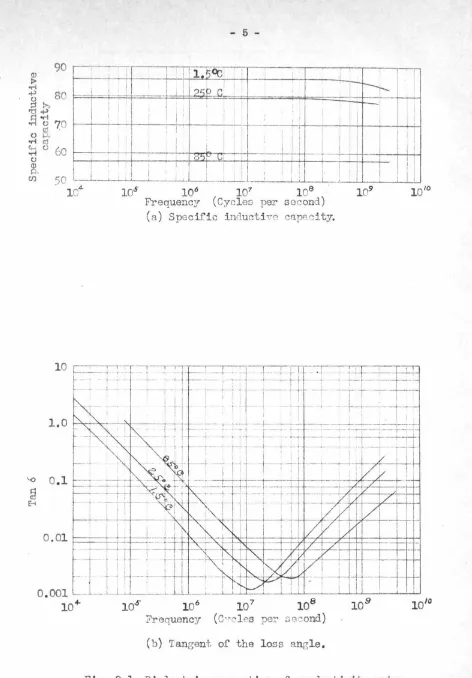
Research1 are plotted in Figs. 2.1 and 2.2.(8,9) These graphs, plus

information from other sources

1

(4~5) indicate that the specific

induc-tive capacities of ice and water at oo C in the range 100-200 megacycles

...

per second can be taken as 3.4 and 88 respectively.

A mixture of air, ice, and water has a permittivity that is not

obtained in a simple manner. A number of formulas have been given for

the permi tti vi ty of mixed bodies. One formula is (r o)

I ..

V,

(2.17)

while another one is

k

v,

k

If lc

£ ...

=

1 £.1 -r-vz. Z-z. (2.18)

where u and k are constants which usually.have to be determined

ex-perimentally.

In

Eq. (2.18)1 V1 and V2 are the fractional part of the

volume occupied by substances 1 and 2 respectively, and k ranges from

-1 for dielectrics in series to +1 for dielectrics in parallel. The

constant k is dependent upon the shape of the particles. The

defini-tion of permittivity is given by

£,.. :::

I

+-

'1-Tr

J

f

d V

_(2.19)

integrated over unit volume1 where P is the polarization per unit

volume and E is the field. Here it is more apparent that the permit

-tivity is dependent upon the shape of the particles.

Wet snow is not just a simple mixture of air1 ice1 and water. It

- 5

---~

I

1 1.~~1 I _I

l

I I

_L _I

-

_{: - - : - I}

. .L I

I I ?tiP r, I

I

--

~ .. .._

I

I I

i

I

I

I I _I - I I

I I

I

I

I

IJ

I

I

I

! _I

!

I

I

I

'I

I I

I I I I

l

I I I

I

I

I

l:l':>.t' LiL I ,.

I

I

;

I I _{I I}

I

I

I I I I I

I

-

1 I

l

O

s

10

6

₁

₀

7

₁

₀

8

Frequency (Cycles

per

se

c

ond)

(

a

)

Specif

i

c

in

d

ucti

ve

capPcity

.

1

0

106 107 108

7req

uenc

y

(

C-,C'

l

P-

s

per

se~ond)

(

b

)

T

an

ge

n

t

of

the

lo

ss a

n

g

le

.

[image:9.540.44.516.18.696.2]

- 6 - 0

7

1 :

II

' I

_I

II

I

I

! :

I

I

I

_I

I I I

i

I

' I

i

' I

~

I I I

I

I

t---h

_'- I ' I

I

:

r

~

1-- ;

_-

_l20

₁

I I I

l

I

i

I

I;

I

I

I

; I I

106 107 108 109

Fr

eq

u

e

n

c

y

(Cycle~

pe

r

s~cond)

(~)

Spe

cif

i

c

i

nd

u

c

t

i

ve

c~pacity.

I l - I

0.001

--~

-t<1-!

1

r+

~:~

-

---+----0.0001 I I I I

lOs 106 107 108 109

F

re

q

u

e

nc

y

(

C

y

c

l

a

s

per seco

n

d

)

(

b

)

Tange

nt

o

f the l

o

s

s

a

ng

l

e

.

7

-crystals are hexagonal with indexes of refraction of 1.309 and 1.313

at the optical frequencies. There is some evidence to indicate that

the permittivity of snow is influenced by the orientation of the

crys-tal axis.(ll) Gerdel, at the Central Sierra Snow Laboratory, has

obtained agreement within 25% between observed and calculated values

of the permittivity for wet snow using values of 3.0 and 80.0 for the

specific inductive capacities, and k= 1 in Eq. (2.18). Fig. 2.3 is a

graph of the specific inductive capacity of wet snow as a function of

density and liquid water content for k = 1, and specific inductive

capacities of 3.4 and 88 for ice and water respectively.

The calculation of the permittivity of a wet glacier is not possible

because the amount of each constituent is not known. Since air will

be present in important quantities in only a relatively thin surface

layer, it is not important. The important quantity is the amount of

liquid water present. The only feasible way to find this is to compare

the delay time for the reflection of electromagnetic waves to the known

depth as determined by some other method. I f the velocity of

propa-gation is found to be constant or is predictable, then radar might be

used successfully for "sounding".

The attenuation of electromagnetic waves in solid ice, calculated

by Eq. (2.09) and the data of Fig. 2.2, is plotted in Fig. 2.4.

Before attempting the propagation of electromagnetic waves in

glaciers, order of magnitude calculations should be made to determine

the maximum range that can be expected. The problem will be set up

with several simplifying assumptions. It will be assumed that the beam

angle is amall enough so that all the transmitted power impinges on the

target, and that the target scatters the reflected energy over a half

sphere. The power received back at the antenna is given by

!;.

;:

/!

L

A~

I

/)

-

6.1.11.~

- 8

-1.00r---~---~---~---~---~---~---~

0. 90 1 - - - - -!

-0. 80 - · - - -- t - -

-0. 70 1 - - - -- -

-$

_~

_0.60

]

p. ;_?;

8

0.50

Cll

~

0 I>.

~ _{~ 0.40}

Q)

0

0.20

-0.10 t - -- - - - 4

. - - -- -- - -·

--+---

---·--+---~-o ~---~---~---~---L---L---~---~

0 1 2

3

4

5

6

7

Snecific inductive capacity

0

.

7

_I

I •

I

i j I I I 1

I

i

I

!

I

!

I

I

I

o

.

6

r

~

__

• _

1

I

1

!

1 . I

rT

I

:

-~

-

I -· .

.

I

' '

I

i I

1 ' I-I r I , 1 •

I

'-· I

~

I

~

0

.

5

-~ (J)

s

I

A

!

~

0

.4

~-~ (J) ~ C) <D p .._,

l=l

0

.

3

0 -rl

~

_,

-

·-~

r-f T

i

I-t----

_I

--~

I

j_

- ~ - -1

i

i :- 1 I I l

t----i--ll----~- II

ri---

----~

-~--1----.---f---1 ' I I I

E

<D

~ 0.2 <

I i I

I

I

I I ;

I

I

I I I

I ! I I J '

I

_j_ _

____l

! .

:

l I - - - - , - -+-+--Y

I

.

I I

0.1

I

j

+

-'

I

-120 C 1 I

1

l

-

_/I

I I

I

I

t-I

I

!

!

I _l

I

I . -•

-r

~

I

I

---1--

t

1_

--r-·

1

I

I

I

I

)

r ---

·

--

-·

--!

I

I

I

I

I I

i -- - - !

!

I _{• I I}

107 109 109 1010

Frequency (Cycles per s~cond)

Fig. 2.4 Attenuation of electromagnetic waves in ice.

10

-where Pt is the transmitted power,

R is the reflection coefficient of the target,

r is the range,

Ar

is the receiving antenna effective cross section,

~ is the attenuation constant in decibels per unit distance.

If a frequency of 180 megacycles per second is selected, minimum detec-table power is assumed to be lo-13 watt, and other values applicable

to the equipment to be used are substituted into Eq. (2.20), this gives

(2.21)

Solving this gives a value of a little over 600 meters, or approximately

2000 feet, for the maximum range. This looks promising since many

glaciers have lesser depths. The moat important thing that was taken

for granted was the reflection coefficient of the bedrock floor. At

these frequencies, rock acts as a dielectric in so far as its reflecting

properties are concerned.(l2) It is entirely possible that the

permit-tivity of the rock might be the same as the ice just above it.

In Eq. (2.20) the damping factor, not the inverse square of the

distance, plays the dominant role in determining the received power.

If the value of r in the inverse square factor is assumed constant,

the solution of the equation for the maximum range gives

(2.22)

where Pmin is the minimum detectable signal. The values just used are

now substituted into Eq. (2.22) plus the value of 600 for r. This gives

From this, one can obtain an idea of the importance of the factors in

- 11

-factor of 21%.

I f the liquid water content at some place increased very slowly

with distance to a large value, there would be little reflection of

energy. The waves would just continue to propagate at a lower velocity.

One might think that the range of the most distant echoes would tell

whether the energy had been propagating through ice or water. However,

calculation of the attenuation in conductivity water shows that it is

approximately ten times that of ice at these frequencies. Since the

ratio of the velocities of propagation is also nearly ten, the maximum

delay times to be expected would be the same for propagation in either

medium.

The method of introducing the energy into the ice must be

con-sidered. If the antenna is submerged in the neve, or a parabolic dish

antenna is placed face down on the surface, then all the energy must

go into the ice. I f the antenna is some distance above the surface,

some of the energy will be reflected. If the antenna is a great

dis-tance above the surface, the reflection coefficient is given by Eq.

(2.16) and for an ice-air boundary would be less than 10%. Since the

antenna will always be close to the ice, the rigorous solution must

be worked out to get the an~er. However, as shown by Eq. (2.23), a small amount of power lost is not of much importance; the more

impor-tant consideration is the antenna field pattern.

An antenna in region 1 has a beam angle in degrees between half

power points of approximately(l3)

:J.8, ~ ?~A,

(2.24)

where ~. is the wave~ngth in region 1 and d is the dimension of the

antenna in the plane where the field pattern is taken. This is only

a good approximation for d

>

2

A,

.

Again, considering the case where

- 12

-1 and 2, Snell's law of refraction is

{l,

~

!},

=

(Z

~

B:~-For small angles this oan be approximated by

Bz

~

/3,

ff,

V£;

giving as the beam angle in region 2 as

:1

Bz.

~

:J..

e,

If

3<'

7() ).,

J

(2.25)

(2.26)

(2.27) When an antenna of the same dimension is operated in region 2, the change in wavelength is given by the formula

(2.28)

Therefore the beam angle in region 2 is

7

o>.,

d

(2. 29)

which is the same as Eq. (2.27). This may indicate that the physical

size of the antenna determines the beam angle in region 2 regardless of which region the antenna is located in. To get the exact field

pattern when the antenna is close to the ice requires the rigorous solution of this boundary value problem, but this would be extremely

tedious. Even the case of a single oscillating dipole above the

sur-face of a complex dielectric (earth) has received a great deal of attention from Sommerfeld and many others since 1909.(14)

It is obvious that the presence of ice in the local fields of the

antenna will affect its input impedance. This can be taken care of by

suitable matching methods. It is not necessary to know the input

13

-III. PRELIMINARY CONSIDERATIONS IN THE SELECTION OF EQUIPMENT

The first consideration should be given to the choice of frequency.

The upper frequency limit is set by the increased attenuation of the

waves in ice (Fig. 2.4). There are several factors which govern the

lower frequency limit. For a given beam angle of the radiation pattern,

the physical dimensions of an antenna vary inversely with the frequency.

Considerable directivity is desirable so as to minimize echoes from

the side, such as those from crevasses. If the beam angle is large,

a horizontal discontinuity will give back a broad echo unless there is

specular reflection. The increased antenna gain resulting from a small

beam angle also increases the maximum range somewhat.

The choice of frequency is also correlated with the choice of pulse

length. The length of pulse selected will depend upon whether the main

interest is short minimum range or long maximum range. Even if it is

the latter, too long a pulse cannot be allovred, because fairly good

range resolution is necessary to separate the multitude of echoes that

reflect back from a glacier. This also sets a lower frequency limit

because it is difficult to generate a pulse of only a few cycles duration.

However, the limit set by antenna size will usually be more important.

The choice of power output is not particularly difficult to make.

As shown in Part II, a large increase in power output will not increase

the range by a very great factor. The maximum size of the transmitter

is governed by the amount of weight that can be tolerated. This is

important because the equipment will usually be transported manually.

With the exception of the power supply, the only part of the equipment

whose weight will depend upon the power output is the transmitter.

Therefore, there is very little point in conserving weight by making

the transmitter extremely small. On the other hand, i f the advantages

14

-that it contains a major portion of the total weight. Between either

extreme there is plenty of latitude for a reasonable choice, and a

transmitter which weighs one-fourth of the total weight seems like a

15

-IV.

1948 EXPEDITION

(a) Location and Equipment

During the summer of 1948, experiments were conducted on the upper

Seward Glacier to determine the applicability of radar methods to the

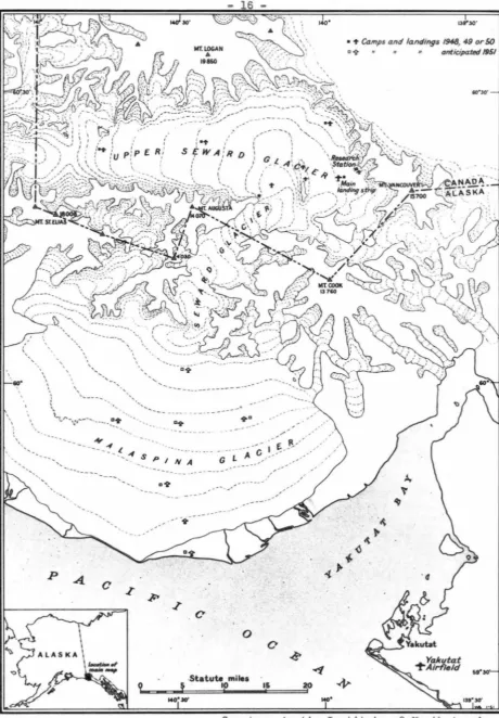
problem of finding the depth of a temperate glacier. The base of

opera-tions was located about sixty miles north of Yakutat, Alaska in the St.

Elias Mountains, Yukon Territory. Fig. 4.1 is a map of this region.

The equipment used was a modified SCR-718-A pulse type radio

altimeter. Since the attenuation at the original frequency of 440

megacycles per second was thought to be too great, the original trans-mitter and mixer assemblies were removed and replaced by similar ones

designed for 100 megacycles. This equipment had been designed to use

separate transmitting and receiving antennas and it was decided to use

the same arrangement.

The pulse repetition frequency, 98.356 kilocycles per second, was

unusually high for pulsed radars. The information was presented on

a cathode ray tube with a circular sweep of the same frequency. The

air range corresponding to this frequency is 5000 feet. The output

pulse originally was of 0.25 microsecond duration. This was lengthened

to 0.4 microsecond. The peak power vms approximately five watts.

The original equipment, being airborne, was designed to operate

from 115 volt, 400 cycle current. In the aircraft, this was supplied

by an inverter which, in turn, was supplied by a gasoline driven

generator. The same method was used in the field.

The transmitting and receiving antennas were made identical.

Each was a two-by-two broadside array of half-wave folded dipoles as

shown in Fig. 4.2. The dipoles were submerged a quarter wavelength in

the neve and the surface covered with a mesh screen to serve as a

'

' _' ' '

'

.

' ' L~---...._

'.. ·.

'-

v'-,.-

,--

-

-

-

---

-

~!

p

\

i

\ \

\

,,__.,

~

,..,..,

~

.

•

·~·-.

___ ..

0

.statute miles

lp

0

1,6 2,0

100.

• ~ Camps and landings 1948, 49 or 50

o ~ anticipated 1951

60"30'

Courtesy Arctic Institute o~ North America

[image:20.545.57.517.39.700.2]

- 17

-~~

72 ohm Twinex

~

\

JOO ohm Twinex

---

...

~~r<

~

)

\

-

---

~

\

·

~

ll

·

~-~~

~~.I

[1

--_ ----

_

-

--1-::-_-

.

.=::::::...

-

-.:

~

1---'

~-

t

---

~

Fig. 4.2 Schematic of antenn~ use1 in 1948. A mesh screen

18

-with the liquid water content. However₁ the antenna was designed for

a specific inductive capacity of 2.5. Twinex was used so as to

elimi-nate the balanced to unbalanced transformers which would have been

necessary with coaxial line. The characteristic impedance of the Twinex

was chosen to match the radiation resistance of the dipoles₁ which was

estimated from the data available in the literature.(l5,16,17) Bal-anced feeding of antennas is most satisfactory for broad-banding.

Sufficient broad-banding was assured by using heavy elements and folded

dipoles. The antenna patterns are shown plotted in Fig. 4.3.

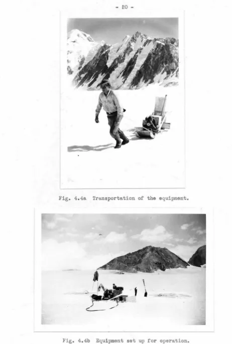
The entire equipment was transported on an Army four-man arctic

sled (Fig. 4.4a). The setup is pictured in Fig. 4.4b. (b) Operation and Results

"Soundings" were first attempted on the main part of the upper

Seward Glacier. Nothing consistent that looked like bedrock was found,

so it was decided to work on something shallower. Later soundings by

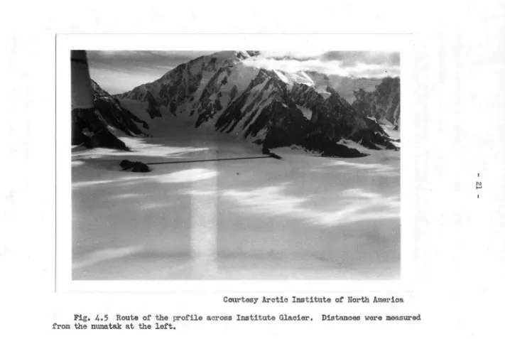
seismic methods showed that this first location was about 2200 feet deep. The next set of locations was made on a small valley glacier at the eastern edge of the upper Seward Glacier proper, which was chris-tened "Institute Glacier" by the members of the expedition. The route

of the transverse profile is shown marked in Fig. 4.5. It ran from the

research station on a nunatak in a southeastern direction to a mountain

ridge (Fig. 4.1). Stations were spaced at approximately 500 foot

inter-vals. So many echoes were received that their identification was quite

uncertain. At some of the shallower stations two or three echoes were

received equally spaced in time, and these were believed to be caused

by multiple reflections. I f it is assumed that reflection from a ho ri-zontal layer of dielectric discontinuity in the ice is more specular

than that from the bedrock, then the echoes from bedrock should be

19

-8

(a) Field

str

ength

pattern

in

p

lane

para

llel

to dipoles.

(b)

Field strength

~ttern in

plane perpendicular

to

dipoles.

20

-Fig. 4.4a Transportation of the equipment.

\

t

j

-z , - - .

[image:24.564.48.510.41.727.2]

Courtesy Arctic Institute of North America Fig.

4. 5

Route of the profile across Institute Glacier. Distances were measured from the nunatak at the left.

[image:25.760.41.752.41.518.2]

N

22

-curve of the apparent profile. Other considerations were that it must be continuous and the depth at each end be zero.

From the data taken, the curve of Fig. 4.6 was obtained. The

depths shown are the equivalent air ranges and must be corrected for

the velocity of propagation. It is of interest to note that the

maxi-mum range echoes were usually received at equivalent air ranges near

2000 feet, since this was predicted in Part II.

After the equipment had been operated for several days it became

evident that there was room for improvement. One of the main

disad-vantages was the time necessary to take a reading. · Under average

conditions, only one station could be covered each day. This was because of the condition of the snow surface. A crust would usually

freeze each night which was firm enough to support men and sleds.

This would remain until about ten o'clock each morning. Until then the

sled could be pulled by one man, and the best time to move the equip-ment was just before this crust melted. By that time the trenches for

the dipoles could be dug quite easily. The complete operation of

moving 500 to 1000 feet, taking a reading, and repacking took one man

three to four hours. After that there was nothing to do but wait until

the next morning for another frozen crust.

A considerable amount of time was necessary to install the antennas in the neve. If an antenna that could have been placed above the

sur-face had been used, much time would have been saved. Regardless of the type of antenna, one for both transmitting and receiving would have

saved both weight and time. (c) Other Methods

Two other parties of the same expedition also attempted to measure

the glacier depth. One group was from the National Research Council

- 23

-- I

_-f

-

1

--

-+

-

,

-

§

I

1

I

I

I

I

I

I

I

I

I

.

tO

. I

--

+---t-

§

~

- · - - _gj

lJ"\

I ,--.. ~

I

I

i

I

+l ~

i

Q) Q) ~

I

I

1%. ~

I I ... ~

-

-·--

-

1

_-

-~

§~

_~

(I)

~

I

~

'S

I _.!=!

V)

I

.s

:!:

s

~ 0 .0

I

gt

0

\.{)

--r

.

l~--

~

---

-

-·t-

-

Q)

O<D r-1

~~

•rl

! I ~

I

0

Ill

k

I

•rl 0

...0

I

.

8

...;t

- -

-

,-0

.

C\! _~

r:.

~--~--~--~--~---L---L--~--~0

0

§

§

r-i C\l

24

-sound waves to reflect from the bedrock. The frequencies used were

in the sonic range, extending from 100 cycles to 16 kilocycles per

second. Bandpass filters enabled them to select the frequencies desired. A pulse of sound waves was obtained by detonation of an electric blasting

cap designed for seismic use. Much difficulty was experienced in

se-curing satisfactory geophone coupling and in transmitting a sound wave

to the solid ice below the neve. Probably most of the explosion

ener-gy was dissipated in the immediate neighborhood of the charge.

Consequently, no profiles were obtained and the technique, in its present

form, was deemed unsatisfactory for the upper Seward Glacier.(l8)

The other party, from the University of Toronto, experimented with conventional seismic equipment. Although this method had been proven on bare ice glaciers, the same difficulties were encountered that were mentioned above for the sonic method. Echoes from bedrock were finally obtained at one location by placing the dynamite in a

- 25

-V. GLACIOLOGY

The upper Seward Glacier is a relatively flat intermontane glacier

of over 500 square miles area. There is an excess of accumulation over ablation of snow each year and the surplus flows out through a gap

three miles wide. There is very little precipitation in the summer.

The excess accumulation averages about 30 inches of water per year, but the precipitation for the winter of 1948-49 was estimated at 80

inches with a net accumulation of 69 inches.* Melting was sub-normal during the summer of 1949.

The density of the neve ranged from close to 0.50 at the surface to 0.85 at a depth of 50 feet. Horizontal blue ice bands vrere spaced

at irregular intervals, but averaged every few feet. These had densi-ties around 0.90 as compared to solid ice with a density of 0.917.

Vertical columns of large ice crystals, loosely bound together and

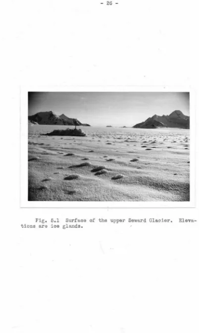
usually less than eight inches in diameter, extended between the ice layers. Most of these ended at ice layers. These are known as ice

glands (Fig. 5.1).

The daily meltwater vreve percolated downward at initial rates

between 6 and 8 inches per hour. This rate became less as it progressed, the meltwater maximum descending the first 10 feet in 24 hours. The greater the depth, the more continuous is the meltwater flow. The

largest amount of meltwater collected was 0.17 cc/ cm2-hr.

In 1948, standing water was found in several crevasses in the

central part of the upper Seward Glacier at depths .of 60 to 70 feet. One hole was bored by an electrically heated hotpoint to a depth of over 200 feet. The drilling rate for the upper part was 1.6 minutes

• The study of the physical characteristics of the glacier was carried out by a group of geologists under the supervision of Dr. R. P. Sharp

26

[image:30.543.70.472.45.717.2]

- 27

-per foot. At the water level in the neighboring crevasses, this rate

decreased to 8 minutes per foot. Since the heat conductivity of water is approximately one-third that of ice,(20) this change might be

ex-plained by loss of heat due to convection. This would indicate that

there is a water table, and that the liquid water content is greater

below this level. However, in 1949, standing vmter was not found in

crevasses that were penetrated to nearly 100 feet in depth. This

disappearance or depression of the water table was probably due to the fact that the summer of 1949 was much cooler, so ablation was less.

Crevasses probably do not extend much more than a hundred feet in depth in any glacier.(21) Below this depth the pressure would keep

any from forming, or plasticity is so great that those which do form

close up quickly.

After the winter cold wave had dissipated, the temperature down to a 200 foot depth was found to be at the melting point, and presumably

28

-VI. 1949 EXPEDITION

(a) Equipment

Experiments were continued in 1949 on the same profile of the

Institute Glacier. The receiver and indicator were retained from the

1948 equipment but the rest of the equipment was different. A frequency

of 180 megacycles per second was used because of the availability of

transmitter, antenna, and receiver RF section.

The transmitter was a BC-1072-A, a component of the Signal Corps

IFF equipment RC-148-A. The pulse length was shortened from 10 to 0.5

microsecond and the output was changed from balanced to coaxial output.

Peak power was approximately one kilowatt. An AN-154-A antenna vms

used. This is the antenna for RC-145-A or RC-184-A IFF equipment, which,

in turn, is associated with Signal Corps radar equipment SCR-545-A and

SCR-584-A respectively. The only changes made were removal of the

lobe switching device and a slight modification of the RF feed (Fig. 6.1).

The antenna pattern is plotted in Fig. 6.2. This would be the pattern

if it were operating in air and must be modified due to the effect

of the ice. The RF section of the receiver was obtained from a BC-701

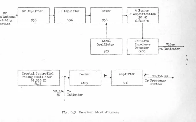
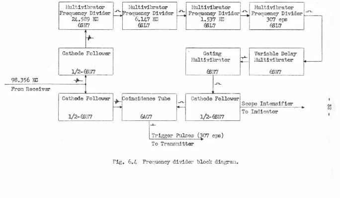
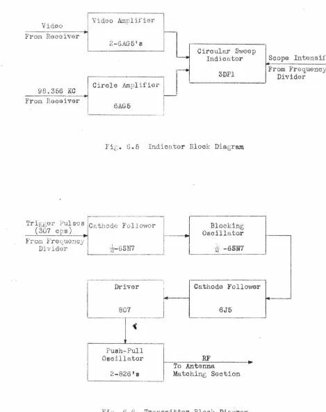
receiver. Block diagrams of the equipment are shown in Figs. 6.3 to 6.6.

Transmitter and receiver were connected to the same antenna by an

antenna matching section taken from the BC-1267-A (the

transmitter-receiver of the RC-145-A or RC-184-A). The purpose of this matching

section was to guide all the transmitted energy from the transmitter

to the antenna, and all the received energy from the antenna to the

receiver. The principle is as follows: The transmitter, when not

oscil-lating, looks like a pure reactance. I f the distance from the transmitter

to the junction is the proper length, the returning energy will see

infinite impedance in the direction of the transmitter and, hence, will

Transmitter

Stub

Tuner

Ill

Antenna f.fatching

Section

•

Receiver

F~.

6.1

Schematic of antenna used in

1

949.

Reflector_

t

¥

1;

!\)

- 30

-{a) Field strength patter~ in plnne perpendicular to dipoles.

-~-

\

--\

I

-(b) Field stren~th pattern in TJlnne pnrallel to dipoles.

RF RF Amplifier RF Amplifier Hixer

1-- ~

From Antenna

l1atching

956

956

956

C' --~ ..

-Local Oscillator

955

..

Crystal Controlled _Peaker

,.._

Timing Oscillator ~

98.356 KC

6AG5

6AG5

.

98.356 To

KC Indicator

Fig. 6.3 Receiver block diagram.

6 Stages

r--.

IF Amplification

30 1·£

6-6AG5's

Infinite

Impedance Video Detector _{To Indicator}

6AG5

-Amplifier

Jl-98.356 KC

61.6

To Frequency _Divider

[image:35.729.32.714.70.494.2]

~

Hultivibrator

Frequency Divider

24.589 KC

(:SN7

f+-Cathode Follower

l/2-$U7

98.356 KC

+-Fro~ Receiver

Cathode Follmrer

1/2-(:SN?

Hultivibrator Multi vibrator Hultivibrator

-"'-Frequency Divider .J"L. Frequency Divider ..J""- Frequency Divider

-

-

~

6.147 KC 1.537 KC 3Cfl Cp:!

f£L7 (:SL7 $17

Gating Variable Delay

Hultivibrntor _1--

+

Hultivibrator

ffi:N7 (:SN?

-l"'---.

~

~oincidence Tube -r-... Cathode Follower _{Scope Intensifier}

f4-

__,__.

To Indicator MG7 1/2-ffiN7

~

Trigger Pulses (307 cp:!)

L _ _ _ _ _____ . . .

To Transr:d tter

[image:36.757.39.723.81.479.2]

Fig. 6.4 Frequency divider block diagra.n.

...

I

I

c.;

- 33

-Video Video Amplifier F'rorn Receiver

r--2-6AG5'a

L.-.., Circular Sweep

Indicator Scope Intenaif ier

r--+

3DP1 From Frequenc_Divider y

98.366 KC Circle Amplifier

r---From Receiver

6AG6

- _J

Fib. 6.5 Indicator Block Diagr~

Trigt;er Pulses _{Cathode Follower Blocking}

(307 cps) _Oscillator I<'rom Frequency

~6SN7 ~ -6SN7

Divider

-

-

---

-.--

-Driver Cathode Follower

807 6J6

Push-Pull

Oscillator RF To Antenna

2-8261 ; Matching Section

[image:37.555.44.513.71.663.2]

34

-transmitter is oscillating, it is matched to the line. At the start of oscillation, the coupling capacitor to the input of the receiver

will charge up, and henceforward the receiver will look like a pure

reactance. With the proper length of line this will be transformed to

an infinite impedance at the junction, and all the transmitted energy

will go to the antenna. A second matching section was used at the antenna as a stub tuner.

(b) Operation and Results

It had been hoped that with the improved techniques, radar sounding would be rapid and accurate so that much beneficial information on the topography of the bedrock floor could be obtained. As readings were taken at the stations on the Institute Glacier profile, it became apparent that the data were as confusing as in 1948. After most of the stations had been covered--the two remaining ones involving much

labor because of the hillside they were located on--it was decided that the remaining time could be used to better advantage by

experimen-ting with various techniques rather than collecexperimen-ting

a

host of data on other parts of the Seward Glacier.

The technique that had been used was suspension of the antenna above the surface as shown in Fig. 6.7. Various heights were tried. Because the beam angle was different in the planes parallel to, and

perpendicular to, the direction of polarization, rotation of the antenna should have produced a change in the magnitude of any echo received from a target not on the axis of rotation. On the other hand, a target

on the axis should have remained constant in magnitude. This assumes

- 36

-crevasses. Almost all the echoes changed some when the antenna was

rotated, so that any amount of data desired could have been obtained

by taking a reading every few degrees. However, only two sets of

readings per station were taken, the ~vo antenna positions being at

right angles to each other. The two directions were arbitrarily chosen

as polarization parallel to, and normal to, the direction of glacier

flow.

In order to investigate the polarization of the echoes, an auxiliary

antenna, Fig. 6.8, was constructed in the field. This antenna was used for receiving. The transmitting antenna was directed horizontally in

the direction of a nunatak. By rotating the receiving antenna, it was

established that the echo was polarized in the same direction as the

transmitted wave. The transmitting antenna was then directed downward.

Trouble was experienced in getting a unique display, as the presentation

even changed with motion of the receiving antenna parallel to itself.

However, the echoes seemed to have no preferred direction of

polari-~~

zation. Due to the dissymmetry of the receiving antenna, quant~tive

~~

information could not be obtained and the qual~tive data just mentioned

are questionable.

The profile was again retraced, taking four sets of data at each station. The four sets consisted of readings with the four possible

combinations of the two antennas polarized parallel to, and perpendicular

to, the direction of glacier flow. The various sets of data were not

very consistent; nevertheless, the six sets of data at each station

were superposed, and after giving each echo due weight according to its

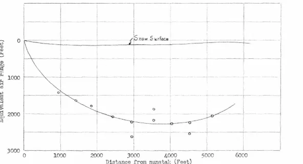
size, appearance, and consistency, the curve of Fig. 6.9 was selected

as the most probable. The points plotted are the locations where good

echoes were most consistent. Again, these depths are equivalent air

'

j_

I

- I - -

I

I

-

1--:;;-

~

~

0 I

i

_'

- - I

[image:41.723.61.653.91.412.2]

~

...

~

§

_~

- -

-+---

_.

-.!1

1000

i

-,--

. ·

---

---

---,.---a:

1l

I -·- __ _,__

--~

I

:

~

til --- I

'

I

> ---'

..-i ' - - - - --- .L

g.

2000

rx:l

'

;

I

i

-

---- -

-r- -

---~---~

Js11ow...S .14 rfdCa ________

-~

_ _ _ _ _ t _ _ __. ____

j

I I

i

I

! ---~

---+-1 o - - '

/

I

~~ ----I

r-1 0 3000 0 I

I

- - - L - -

0

1

- - - [

-o-

--~

--1000 2000

3000

4000 5000

---6000

Distance from nunatak (Feet)

Fig. 6.9 Prof'lle obtained by radar in 1949.

CJ.l

- 38

-year~ maximum range echoes were usually received at equivalent air ·ranges near 2500 feet.

One of the most distressing phenomena was the change with time of the echo display~ even when the equipment had not been touched. It

was first suspected that the temperature of the equipment was responsible.

Therefore a series of experiments was conducted to determine the cause

of this anomaly. 'I'he conclusion was that it was caused by something

external to the equipment, presumably by percolating meltwater in the

glacier as discussed in Part V.

Velocity of propagation measurements were made in the surface layer

of the glacier. This was done by placing the antenna and a target in

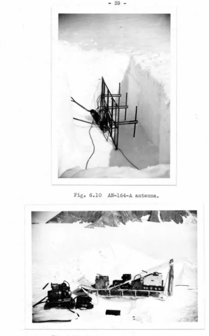
trenches 545 feet apart. The antenna in its pit is shown in Fig. 6.10~

and the rest of the equipment in Fig. 6.11. The echo received was very

large, showing that attenuation was no problem for distances of this

magnitude~ at least for propagation in the surface layer. The

equiva-lent air range of the target, as determined by radar~ was 910 feet.

This gives a specific inductive capacity of

f..'=

((flO\=

;J. j

S4-S)

(6. 01)

Referring to Fig. 2.3, and assuming a density of 0.50~ the liquid water

content is seen to be 1.2%. This is within the limits as determined

by other methods.

The biggest improvement in technique over that of the previous year was operation of the antenna from above the surface. The time to

run a profile took about one hour per station~ most of which was spent

in taking down and setting up equipment. Stations were approximately 500 feet apart. Surface conditions were usually satisfactory from two

- 39

-Fig. 6.10 AN-164-A antenna.

[image:43.561.69.483.43.710.2]

~ 40

-(c) Other Methods

In 1949~ gravimetric and seismic investigations were carried out

on the upper Seward Glacier.( 22 ) Seismic soundings were successful, but

the charge had to be placed in solid ice some sixty feet below the

sur-face. It was not definitely established whether the necessary depth

depended only upon the ice density, or whether a water table played

an important part. Inasmuch as the drilling rate was about 1.6 minutes

per foot, this part of the operation took from one to two hours. The

receiver geophones were placed on the surface. The average rate of

running a profile was two stations per day. Glacier depth was

deter-mined at five stations on the Institute Glacier. This seismic equipment

was limited to thicknesses of ice greater than about a thousand feet.

The upper Seward Glacier is very favorable for gravity-meter

obser-vations because of the subdued relief of the snow surface~ and the

contrast in density between ice (0.9) and rock (2.7-3.0). Two surveys

were made, one nearly seven miles long on the upper Seward proper, and

the other across Institute Glacier. Under good sledding conditions,

stations spaced 500 feet could be covered at the rate of one every ten

minutes. From the data of gravity surveys, only the general shape of

the bedrock floor can be obtained, not the absolute ice thickness.

However, the ice thickness can be determined at several control points

along the profile by seismic methods.

The ease of taking a gravity survey is offset by the labor and

difficulty of interpreting results, expecially in a region such as

this where no good maps of the topography exist. The topography must

be knovm so that corrections can be applied to the raw data. Not only

is a knowledge of the topography of the exposed land masses necessary,

but also of the topography of the bedrock floor under the glacier.

41

-usually much more subdued. Two-dimensional analysis was used on the

gravity-meter data of the Seward Basin. By trial and error, a profile

was finally arrived at which was in accord with the gravity data.

Analysis of the Institute Glacier data was not made because of

lack of information on the surrounding topography which consisted of

large rock masses in the immediate vicinity. The data were used to

estimate the remainder of the profile obtained by seismic methods.

-7000

~

4000

0

' ' _'

£i

fvo)t)

...

...

r.,.

...

t.

~-- ...

3 r,.vit .S~Y\

1000

- 42

-l5l'lollll SIJY~ tt'-~

j

-!

-.

;

,

-

EJ:-

lt .. .J

-

- fy

ey

-

_.,

v ~.,.,

'y

vtty s rvt.t

"-f:rD.b

.S.~l!. Ill!. r:J.

lta/

2000

3000

4000 5000

6000

Diatanoe from nunatak (Feet)

- 43

-VII. ANALYSIS OF EQUIPMENT

After a small amount of field work had been done in 1948, it became

obvious that the equipment was not performing satisfactorily. Echoes

changed in shape, magnitude, and range when the transmitter output

coupling, receiver input coupling, or local oscillator coupling was

varied, or when the Twinex cables were moved. To test the performance

of the set when operating in the air, two half-wave dipoles were con

-structed and set up above the surface. A nunatak was about 1000 feet

distant. Besides an echo which apparently came from the nunatak, other echoes appeared at ranges where there were no objects, at least not

above the surface. The possibility existed that these other echoes

came back from discontinuities in the glacier.

The components of this equiprrent that were retained for the

suc-ceeding year were the IF strip of the receiver and the indicator.

After the equipment was put in a functional condition, it was tried

out on the roof of Mudd Laboratory. Many echoes were received, some of which could be identified. All echoes changed when the antenna

was rotated in direction, so operation was believed to be satisfactory. It would have been desirable to test it on the desert and to conduct

more laboratory test, but time did not permit.

When field operations were begun in 1949, many anomalies appeared which were strikingly similar to those of the preceding year. Adjust-ments which caused the echo display to change were tuning of the receiver,

transmitter output tank, antenna matching section or stub tuner, and

movement of the antenna. When the an~enna was directed horizontally toward a nunatak or the mountains, other echoes appeared besides those

from visible objects, but again, the possibility could not be excluded

that some energy was penetrating the surface and reflecting from a

44

-identified echoes were quite stable to the various adjustments, while

the others were not. Several times when the set had been tuned up on

identified echoes, the coaxial cable between antenna matching section

and the antenna was replaced by one of different length. This entailed

retuning of the stub tuner, indicating that the line was not flat. The

fact that the coaxial connectors were not the constant impedance type

may have caused some trouble. A slotted line would have been very

beneficial in obtaining optimum performance.

After field operations had been concluded, laboratory tests were

conducted on the receiver to determine its qualifications for the work

just completed.

The requirements for a pulse amplifier capable of handling a large

dynamic range of signals are very stringent.(23) Amplifiers often show

a loss of sensitivity after a very strong pulse of short duration. The

most common cause is collection of charge upon a grid coupling condenser.

Another cause is the Whippany or blackout effect(24) and is thought to

be closely analagous to the anode effect.(25) It is thought that a

thin film of insulating material forms on the grid so that when grid

current is drawn, electrons deposit on this layer and take an appreciable

time, of the order of microseconds, to leak off. There is considerable

variation of the blackout effect, even among supposedly identical tubes.

This effect is most serious in the case of video amplifiers and plate

detectors where this apparent change of grid potential shows up as a

spurious signal instead of a change in gain, but the decrease in

sensi-tivity is also an important consideration in high-level bandpass amplifier

stages.

Probably the greatest cause of trouble in the receiver was the

fact that the incremental gain of each IF stage was negative at the

- 45

-output signal. The incremental gain is defined as the slope of the

curve obtained by plotting input against output.(26) Such a curve is

shown plotted in Fig. 7.la. I f the input of a stage is a signal which

increases with time as in Fig. 7.lb, then the output will be the curve of Fig. 7.lc. Now if a second stage is connected to the output of the

first stage, its output will be the curve of Fig. 7.ld. This can be continued for each additional stage added; the result is a hump for each stage. Of course, a decreasing signal will give a similar effect, so a large echo with a slow rise or decay time will appear as a number of echoes.

This performance was verified by observing the response of the

receiver to RF pulses of various magnitudes and durations. When the

IF stages were overloaded with a RF signal modulated by a sine wave, the hills and valleys interchanged as the gain was increased. The

response of the video amplifier fell off too much for the lower

fre-quency components of the pulses, and overshoot was excessive. A five-microsecond, two-millivolt pulse fed into the IF strip decreased the

sensitivity considerably for a period of thirty microseconds.

The method of gain control is also important.(27,28) Reduction of

plate or screen potential lowers the saturation level and should never be used when overload capability is of importance. The best way is

to return the grid circuits to a variable negative voltage supply of low impedance for quick recovery from overload. The slight amount of

detuning caused by change of bias will usually not be of importance, expecially in wide-band amplifiers. I f the gain variation must be large, several tubes should be controlled so that none will be biased to cutoff.

The method of gain control for the receiver under discussion was

r

-!-)

:::i ~

-0

~

I

--~-

!

-

-

!

-

~

,

r_l

t1

~-

j

_

_

_~

'

/ I

~ _ _ J _ _ _ _ _ _:::..,. _ _

Em-~

(a)

Output

vs.

input.

I

f----1---+--"

~

r2

Time ;.

(d)

Output of second stage.

-L-1

+

_I

-

--1 :

_t--

_.

,

1

fl

+

I

f

~ +---I ~

--+-

g

rx::l _rx::l

T i m e - --> Time :>

(b) Input of first stage. (c) Output of first stage.

Fig. 7.1 Behavior of two stage lllilplifier i f incremental gain

is negative when input signal is equal in mac;nitude

to

output sig

-nal. All voltage scales and All time scales are the same.

"""

[image:50.758.2.754.22.525.2]

- 47

IF stages. The IF stages were double tuned.

Certain requirements are necessary for a second detector for pulse

reception.(29) It should have high gain6 be reasonably linear, have

good transient response, be capable of handiing large signals₆ and not

load the IF amplifier too much. The diode detector fulfills all these requirements except the first and la~t, and so is used most widely for

radar receivers. In wide-band amplifiers, IF amplifier loading is usually not a disadvantage, as the stage must be loaded anyway. This receiver used an infinite impedance detector. It has low gain, but its

chief disadvantage is that it is subject to overloading, though to a

lesser extent than the plate detector. These faults probably made little difference because so much damage had been done to the signal before it reached the detector stage.

Measurement of the input impedance of the receiver using a slotted

line and the output pulse of the transmitter showed that that there was no length of the antenna matching section (receiver branch) which would give infinite impedance at the junction. Clearly, this type of

duplexer was not satisfactory.

In brief6 the following suggestions are offered as a guide in the

construction of radar equipment for future work in exploring glaciers:

(1) build a receiver to the most rigid specifications for the

amplifi-cation of pulses covering a wide dynamic range; (2) use a spark gap

duplexer which, of course6 also means a transmitter with a reasonably

high peak power; and (3) provide adequate tuning at the antenna, and a

slotted line detector, so that the transmission line can be tuned flat. As a matter of convenience, the laboratory headquarters should be as

48

-VIII. DISCUSSION

If the equivalent air ranges found in 1948 are multiplied by 0.89

and those of 1949 by 0.581 the curves of Figs. 8.1 and 8.2 result.

Comparing these curves with the depths obtained by seismic sounding, it is seen that both are in good agreement. However, these velocity of propagation factors were chosen so as to make the maximum depths check with the seismic data. It has been assumed that the average velocity of propagation was the same across the profile1 which may not

be exactly true.

I f we had radar data for only one profile1 there would be nothing

wrong with this method. As discussed in Part II1 the only sure way of

finding the velocity of propagation is to work on a glacier of known depth. But whatever the velocity of propagation was, it should have been approximately the same for both years. The difference in frequency is a negligible factor. The liquid water content may have changed, but there was less melting in 1949 than in 1948, so the equivalent air ranges should have been smaller.

Again we encounter an unexplainable situation if we calculate what the specific inductive capacity must have been. Using the reciprocals of the above factors for the indexes of refraction gives 1.26 and 2.98 for 1948 and 1949 respectively. These are both les.s than that of solid

ice without any liquid vmter. I f the data of 1948 are discounted, and

the velocity of propagation used for the seismic waves is assumed to be six or seven per.cent too high, the 1949 radar and seismic curves

agree1 provided the glacier was dry. However1 this is clearly an ad

hoc hypothesis--the radar data are not substantial enough to justify questioning the seismic data.

- 49

-7000

I

· - - -

- -

,

__

-

-

-·-

- - -

-

~~

JlCIW

5~.t.rfi ce

-

-~

;

I

-"'

_1_

~, I

·-~

1 - - -

-

---·r-·

--

- -

- -

~ _t~

~

_~'--

_'

_v

_I

h

_ j _

o

_Y

l

'

.

-r---

I,

f - -

-

-

. -

_-

_{- -}

_,_

~l_

_-

_·-

,_

I

I

_I

I

j

40000

_l

_QOO

2000 .3000 4000 5000 6000 Distance f'rom nunatak (Feet)

Fig. 8

.1

Radar profile of

1

948

for specific irtductive capacity

of 1.26.

7000

-

~6000 Q) ~ ..._.. Q)

'8

~5000

;ti

<

~

""

!"-.

_...,

~

1-1000

1-S )')ow

Sw

~

1

---t-

1-+-

-

--

1---

1:::----

·

- -

--·-fJ 0

0

~---

-

-·

---

1

-2000 .3000 4000 5000

6000

Distance f'rom nunatak (Feet)

Fi

g

.

8

.2

Radar

profile of

19

49

for specific inductive capacity

[image:53.526.10.511.20.693.2]