Variations on the standard model of the universe

(1)

Thesis by

Kris Sigurdson

In Partial Fulfillment of the Requirements

for the Degree of

Doctor of Philosophy

California Institute of Technology

Pasadena, California

2005

(2)

c

2005

Kris Sigurdson

(3)

(4)

Acknowledgements

If you told me not-too-many years ago that I would be so close to finishing a Ph.D. in physics at

Caltech studying cosmology, I just wouldn’t have believed you. But yet here I am and there are so

many people to thank for sending me on this journey and helping me arrive at today.

Deep in my engineering studies at Simon Fraser University three people emboldened me with the

courage to considered the other possibility. I would like to thank Howard Trottier for, through his

wonderful lectures during the first year of my B.A.Sc and our many subsequent discussions in his

office, inspiring me to imagine the Universe and I would like to thank Leigh Palmer and Anthony

Arrott for their encouragement during that time.

I would like thank Douglas Scott at the University of British Columbia for being so persuasive

on the phone that day in the engineering lab and convincing me to become a summer student in

cosmology. While I don’t know where I would be right now if I had opted to study string theory

instead, I’m very lucky I opted to work with Douglas. He introduced me to the world of cosmology,

the Cosmic Microwave Background, and helped send me off to CITA, the University of Cambridge,

and Caltech amongst other things. But getting to Caltech isn’t even half the story!

Firstly, I’d especially like to thank my advisor Marc Kamionkowski for his advice, encouragement,

and wisdom during the past four years here at Caltech. I can remember many occasions where I

would storm in to his always-open door and explain to him my latest (crazy?) idea. He would always

listen and critique it with healthy skepticism. His comments on physics or otherwise were always

helpful and always correct. I hope over the years I have assimilated some of his good judgment

about which problems and ideas make for timely and important research.

I would like to thank Mark Wise for letting me be an unofficial member of his group, and for the

many enlightening and thought-provoking discussions I had in his office about high energy physics.

I would like to thank my collaborators during my time here at Caltech, and especially those who

contributed to the work presented in this thesis: Robert Caldwell, Asantha Cooray, Michael Doran,

Steve Furlanetto, Andriy Kurylov, Stefano Profumo, and Piero Ullio.

I would like to thank the members of the TAPIR and Theory groups at Caltech, and especially

everyone in Marc’s cosmology group. Thanks to JoAnn Boyd, Carol Silberstein, and especially

(5)

Last, but not least, I would like to thank all my friends here at Caltech for their support,

en-couragement, conversations, and diversions over the years: Anura Abeyesinghe, Lotty Ackerman,

Igor Bargatin, Daniel Busby, Songye Chen, Ben Collins, Ilya Mandel, Tristan McLoughlin,

Ali-son Farmer, Paul O’Gorman, Margaret Pan, Elizabeth Jones, Mike Kesden, Ilya Mandel, Karin

Menendez-Delmestre, Mike Santos, Graeme Smith, Tristan Smith, Sherry Suyu, Ben Toner, Lisa

Tracy, Anastasios (Tasos) Vayonakis, Nevin Weinberg, and everyone else I’m forgetting at the

mo-ment.

To my officemate, cosmological beer comrade-in-arms, and (soon to be) senior student Jonathan

Pritchard: Don’t wait for them to install the AC. Get out of 123 Bridge as soon as possible. Get a

window man, you’ve done your time!

To my good friend Alejandro Jenkins: I’ve enjoyed all our conversations about physics and otherwise.

“That reminds me of this episode of the Simpsons.”

Most of all I would like to thank my two best friends here at Caltech, the first people I met, Ardis

(Disa) Eliasdottir and Donal O’Connell. It would have been so different here without you; I don’t

think I could have navigated these waters without you keeping me afloat from time to time. Thank

you so much.

To J, M, and C: Your love reminds me of what is important in this life, and what is just physics.

Dad, Mom, Ryan: I wouldn’t be here without you, without your phone calls from afar, without

your encouragement at every single step along the way, without your patience with me, without

your visits to me at every far corner of the world, without you pointing out those lights in the sky

to me all those years ago.

I would like to thank the Natural Sciences and Engineering Research Council of Canada for

supporting me with PGS-A and PGS-D Postgraduate Scholarships, Caltech for giving me a Special

Institute Fellowship during my first year, and the PMA Division for giving me Teaching and Research

Assistantships. At various points in time the research presented in this thesis was supported at

Caltech in part by DoE DE-FG03-92-ER40701 and DE-FG03-02-ER41215, NSF PHY00-71856, and

(6)

Abstract

In the past decade, due to compelling measurements of the angular power spectrum of the cosmic

microwave background (CMB) radiation, the large-scale matter distribution, the recent acceleration

of the expansion rate of the Universe over cosmic time, and the current expansion rate (the Hubble

constant), cosmology has culminated in a standard model of the Universe. By connecting this

standard cosmological model with predictive theories of physics we can hope to look for signatures of

these theories in the data. Along this line of inquiry we consider in this thesis: (i) the effects on CMB

temperature and polarization anisotropies of spatial fluctuations of the fine-structure parameter

α between causally disconnected regions of the Universe at the time of recombination, (ii) the

suppression of the small-scale matter power spectrum due to the decay of charged matter to dark

matter prior to recombination, (iii) the consequences of a neutral dark-matter particle with a nonzero

electric and/or magnetic dipole moment, (iv) how charged-particles decaying in the early Universe

can induce a scale-dependent or ‘running’ spectral index in the small-scale matter power spectrum

and examples of this effect in minimal supersymmetric models in which the lightest neutralino is a

viable cold-dark-matter candidate. With improved tests and cross-checks of

standard-cosmological-model predictions we can search for anomalies that may reveal the character of the underlying

physics. In this direction we propose in this thesis: (v) a new method for removing the effect of

gravitational lensing from maps of CMB polarization anisotropies using observations of anisotropies

or structures in the cosmic 21-cm radiation, (vi) that measurements of fluctuations in the absorption

of CMB photons by hydrogen in the 21-cm line and deuterium in the 92-cm line during the cosmic

(7)

List of Figures

2.1 The visibility function as a function ofϕ= (α−α0)/α0. . . 15

2.2 The CMB angular power spectrum as a function ofϕ. . . 16

2.3 TheC∂Θ0∂Θ0 l andC Θ0∂2Θ0 l derivative power spectra. . . 21

2.4 TheC∂E0∂E0 l andC E0∂2E0 l derivative power spectra. . . 22

2.5 TheC∂Θ0∂E0 l ,C Θ0∂2E0 l andC E0∂2Θ0 l derivative power spectra. . . 23

2.6 The ΘΘ power spectrum. . . 27

2.7 The ΘE power spectrum. . . 29

2.8 TheEE power spectrum. . . 31

2.9 TheBB power spectrum. . . 33

2.10 The signal-to-noise ratio of the kurtosis due toαfluctuations and weak lensing. . . 37

2.11 The signal-to-noise ratio for detecting theα-fluctuation trispectrum. . . 41

3.1 Density perturbation evolution in the standard case . . . 51

3.2 Density perturbation evolution with decaying charged particles. . . 53

3.3 The matter power spectrum in the standard and charged-decay models. . . 55

4.1 Constraints to the dipolar-dark-matter parameter space [mχ,(D,M)] . . . 60

4.2 Feynman diagrams for annihilation of a DDM–anti-DDM pair to two photons. . . 62

4.3 Feynman diagram for DDM–anti-DDM annihilation to fermion-antifermion pairs. . . . 63

4.4 Feynman diagrams for elastic scattering of an electron from a DDM particle. . . 64

4.5 One-loop dark-matter correction to the photon self-energy. . . 67

4.6 Lowest-order dark-matter correction to the muon anomalous magnetic moment . . . . 68

4.7 Three-loop dark-matter contributions to the EDM of a charged fermionf . . . 69

4.8 Lowest-order dark-matter correction toZ0-pole observables. . . 71

4.9 Photon-exchange contributions to (a)Br(B+ →K+_χχ_¯ _{); (b)}_Br₍_B+ →K+_l+_l−_{). . .} ₇₂

4.10 A typical missing-energy process. . . 73

4.11 Feynman diagrams for photon-DDM scattering. . . 74

4.12 The matter power spectrum including baryon-DDM drag. . . 79

(12)

5.1 The dimensionless linear matter power spectrum per logarithmic interval. . . 91

5.2 Dimensionless matter power spectra forτ = 20 yr andfφ= 1/7. . . 94

5.6 Current constraints on the parameterαs. . . 98

5.7 Lifetimes of a 1 TeV stop, chargino, and stau as a function of mass splitting. . . 102

5.8 Points in the mSUGRA parameter space featuring Ωχ0 1 = 0.11 andmχ01=mτ1. . . 107

5.9 A low-energy parameterization of the higgsino-like neutralino case at tanβ = 50. . . . 109

5.10 Feynman diagrams with four-body final states for the processτe1 → χ10ντff¯0,. . . . 110

5.11 The stau lifetime as a function of the mass splitting with the lightest neutralino. . . . 112

5.12 The spin-independent neutralino-proton scattering cross section. . . 113

6.1 Angular power spectra of the deflection potential as a function ofzs. . . 124

6.2 Power spectra of lensed and delensed CMB B-mode polarization. . . 125

7.1 The D-H, H-H andµ-H thermal spin-change cross sections. . . 132

7.2 The H and D spin temperatures as a function ofz. . . 133

(13)

Chapter 1

Introduction

1.1

The Standard Model of the Universe

In the past decade cosmology has culminated in a standard model of the Universe. The emergence

of this standard model is due to compelling new data from measurements of the angular power

spectrum of the cosmic microwave background (CMB) radiation [1·1], galaxy surveys that have

measured the large-scale matter distribution [1·2], observations of Type Ia supernovae [1·3], which

have measured the relative expansion rate of the Universe over cosmic time, and the Hubble Space

Telescope key project [1·4], which has performed an absolute measurement of the current expansion

rate (the Hubble constant H0). From these observations we now have overwhelmingly compelling

evidence that _∼25% of the energy density of the Universe is in the form of dark matter [1_·5],

∼70% is in a non-clustering negative-pressure component known as dark energy [1_·6] (that acts like Einstein’s cosmological constant [1_·7] and is driving a contemporary period of accelerated expansion),

and surprisingly only _∼5% is in the form of the familiar elements listed on the periodic table and

described by the standard model of particle physics. The geometry of the Universe is now known

to be flat [1_·1], which is presumed to be due to a period of exponential expansion or inflation [1_·8]

that also, through quantum fluctuations in the inflaton field or other fields present during inflation,

created a nearly scale-invariant spectrum of primordial Gaussian density perturbations [1·9] and

gravitational waves [1·10]. These fluctuations have been observed in the angular power spectrum of

the cosmic microwave background [1_·1]. It is believed that, through gravitational instability, these

very same fluctuations grew and seeded the formation of galaxies and the large-scale structure in

the Universe (e.g. [1_·11]). This model forms a consistent cosmological paradigm that has thusfar

been consistent with all cosmological observations and can be used as a baseline to test refined or

alternate theories of cosmology.

While the emergence of this standard cosmological model (SCM) is remarkable, and it is

con-sistent in so far as it describes the observed cosmology, the physics underlying the key unknown

(14)

for a physical understanding of these phenomena and equally importantly look for new ways to test

and constrain this model. By connecting the SCM with predictive theories of physics we can hope

to look for signatures of these theories in the data, and with refined tests and cross-checks of the

SCM predictions we can hope to look for anomalies that point the way to the underlying physics.

This thesis explores both of these lines of inquiry. In Chapters 2–5 physical theories that have

novel predictions for cosmological, astrophysical, or physical observables are considered, while in

Chapters 6–7 new techniques for probing the SCM are proposed. These chapters are self-contained,

stand on their own, and have been presented in chronological order. In the sections below I provide

a brief synopsis of the chapter of the same title including the major results of that chapter, and a

description of my primary contributions to the work.

1.2

Spatial Variation of the Fine-Structure Parameter and

the Cosmic Microwave Background

In Chapter 2, we consider the effects on CMB temperature and polarization anisotropies of spatial

fluctuations of the fine-structure parameterαbetween causally disconnected regions of the Universe

at the time of recombination. Such fluctuations inαmight be expected in theories where the gauge

coupling constants are set by the vacuum-expectation-value (VEV) of a light scalar field.

We first review previous work [1·12, 1·13] that shows how the recombination history depends

on a homogeneous shift in α and then discuss how it affects the CMB power spectrum. We then

discuss how spatial variations of α, in which the mean value of α is unaltered, affect the CMB

temperature and polarization power spectra. Interestingly, we find these effects are analogous to

those of weak gravitational lensing on the CMB, but differ in detail. Like weak-gravitational lensing,

spatial variation ofαinduces a spatially-varying angular power spectrum across the sky. We show

how this has the effect of inducing a curl-mode (B-mode) component in the CMB polarization

pattern. It also induces “non-Gaussian” signatures in the CMB, in the form of locally anisotropic

correlation functions, that cannot be described by the power spectrum alone. We calculate the

CMB bispectrum and trispectrum induced by spatialαvariation. Effects like those we investigate

here may also arise if there are other spatial variations in recombination physics that do not involve

significant density/pressure perturbations. Our calculations are thus illustrative theoretically, apart

from the specific application on which we focus.

In the final section of Chapter 2, we discuss the properties of and constraints to a toy field-theory

model for spatial variation of α that produces the CMB effects outlined above without inducing

significant density perturbations.

This chapter was originally published as “Spatial Variation of the Fine-Structure Parameter and

(15)

Physical Review D68, 103509 (2003). I was primarily responsible for deriving the effects of spatial variation of α on the CMB and writing the technical sections related to that work in the paper.

Kurylov and I worked closely together on the last section of the paper which discusses the toy

field-theory model ofαvariation. Kamionkowski and I discussed the CMB calculation often during the

course of the project, and jointly edited the manuscript.

1.3

Charged-Particle Decay and Suppression of Primordial

Power on Small Scales

While the standard cosmological model is in remarkable agreement with observation, on subgalactic

scales there are possible problems that warrant further investigation. Namely, the model overpredicts

the number of subgalactic halos by an order of magnitude compared to the eleven observed dwarf

satellite galaxies of the Milky Way [1·14]. Several possible resolutions have been proposed to this

apparent discrepancy, ranging from astrophysical mechanisms that suppress dwarf-galaxy formation

in subgalactic halos (see, for example, Ref. [1·15]) to features in the inflaton potential that suppress

small-scale power and thus reduce the predicted number of subgalactic halos [1_·16].

In Chapter 3 we study the suppression of the small-scale matter power spectrum due to the

decay of charged matter to dark matter prior to recombination. In the model discussed, prior to

decay, the charged particles couple electromagnetically to the primordial plasma and participate in

its acoustic oscillations. After decay, the photon-baryon fluid is coupled only gravitationally to the

neutral dark matter. We show how this generically leads to suppression of power for scales that

enter the horizon prior to decay. This suppression, reduces the amount of halo substructure on

galactic scales while preserving the successes of the standard hierarchical-clustering paradigm on

larger scales. For decay times of∼3.5 years this leads to suppression of power on subgalactic scales,

bringing the observed number of Galactic substructures in line with observation. We discuss how

decay times of a few years may be possible if the dark matter is purely gravitationally interacting,

such as the gravitino in supersymmetric models or a massive Kaluza-Klein graviton in models with

universal extra dimensions.

This chapter was originally published as “Charged-Particle Decay and Suppression of Primordial

Power on Small Scales,” Kris Sigurdson and Marc Kamionkowski, Physical Review Letters 92, 171302 (2004). I was primarily responsible for deriving the modified perturbation equations which

include the effects of the charged-decay process, and for writing the initial draft of the manuscript.

Kamionkowski and I discussed the calculation often during the course of the project, and jointly

(16)

1.4

Dark-Matter Electric and Magnetic Dipole Moments

A wealth of observational evidence indicates the existence of considerably more mass in galaxies and

clusters of galaxies than we see in stars and gas. The source of the missing mass has been a problem

since Zwicky’s 1933 measurement of the masses of extragalactic systems [1_·5]. Given the evidence

from galaxy clusters, galaxy dynamics and structure formation, big-bang nucleosynthesis, and the

cosmic microwave background that baryons can only account for ∼1/6 of this matter, most of it

must be nonbaryonic. Although we know it likely exists, we do not know what the underlying theory

of dark matter is or what the detailed particle properties of it are. While theorists have identified

promising candidates for the dark matter, such as the neutralino (the supersymmetric partner of the

photon,Z0 _{boson, and/or Higgs boson) [1}

·17] or axion [1_·18], there is currently no direct evidence that these particles constitute the dark matter. Other candidates are certainly possible.

In Chapter 4, we ask the question, “How dark is ‘dark’ ?” In other words, how weak must the

coupling of the dark-matter particle to the photon be in order to be consistent with laboratory

and astrophysical constraints? In particular we consider the consequences of a neutral dark-matter

particle with a nonzero electric and/or magnetic dipole moment. Theoretical constraints, as well

as constraints from direct searches, precision tests of the standard model, the cosmic microwave

background and matter power spectra, and cosmic gamma rays, are included. Interestingly, we

find that a relatively light particle with mass between an MeV and a few GeV and an electric or

magnetic dipole as large as_∼3_×10−16_e_{cm (roughly 1}_.₆

×10−5_µ

B) satisfies all experimental and observational bounds and remains a phenomenologically viable candidate for dark matter. Some of

the remaining parameter space may be probed with forthcoming, more sensitive, direct searches and

with the Gamma-Ray Large Area Space Telescope.

This chapter was originally published as “Dark-Matter Electric and Magnetic Dipole Moments,”

Kris Sigurdson, Michael Doran, Andriy Kurylov, Robert R. Caldwell and Marc Kamionkowski,

Physical Review D70, 083501 (2004). I computed the dark-matter scattering and annihilation cross sections used throughout the paper and wrote the introductory section on the dipole Lagrangian;

the cross sections were independently verified by Kurylov and Doran. I derived the perturbation

evolution equations for dipolar-dark-matter, implemented them in a Boltzmann code, and wrote

the corresponding section of the paper; these perturbation equations were independently verified by

Doran and implemented in a separate Boltzmann code for comparison. Kamionkowski and Caldwell

completed the relic abundance, direct detection, and galactic annihilation calculations. Kurylov

computed the limits from precision measurements and particle physics. Caldwell and Kamionkowski

(17)

1.5

A Running Spectral Index in Supersymmetric Dark-Matter

Models with Quasi-Stable Charged Particles

In Chapter 5 we show that charged-particles decaying in the early Universe can induce a

scale-dependent or ‘running’ spectral index in the small-scale linear and nonlinear matter power spectrum

and discuss examples of this effect in minimal supersymmetric models in which the lightest neutralino

is a viable cold-dark-matter candidate. If all of the present-day dark matter is produced through

the late decay of charged next-to-lightest dark-matter particles (NLDPs), then, as discussed in

Ref. [1_·19], the effect is to essentially cut off the matter power spectrum on scales that enter the

horizon before the NLDP decays. However, if only a fractionfφ of the present-day dark matter is produced through the late decay of charged NLDPs, the matter power spectrum is suppressed on

small scales only by a factor (1−fφ)2. This induces a scale-dependent spectral index for wavenumbers that enter the horizon when the age of the Universe is equal to the lifetime of the charged particles.

What we show in this chapter is that, for certain combinations of fφ and of the lifetime of the charged particle τ, this suppression modifies the nonlinear power spectrum in a way similar (but

different in detail) to the effect of a constant αs ≡ dns/dlnk 6= 0. Although these effects are different, constraints based on observations that probe the nonlinear power spectrum at redshifts of

2 to 4, such as measurements of the Lyman-αforest, might confuse a running index with the effect

we describe here even if parametrized in terms of a constantαs. This has significant implications for the interpretation of the detection of a large running of the spectral index as a constraint on

simple single-field inflationary models. The detection of a unexpectedly large spectral running in

future observations could instead be revealing properties of the dark-matter particle spectrum in

conjunction with a more conventional model of inflation.

While, even with future Lyman-αdata, it may be difficult to discriminate the effect of a constant

running of the spectral index from a scale-dependent spectral index due to a charged NLDP, other

observations may nevertheless discriminate between the two scenarios. Future measurements of the

power spectrum of neutral hydrogen through the 21cm-line might probe the linear matter power

spectrum in exquisite detail over the redshift range z _≈ 30₋200 at comoving scales less than 1

Mpc and perhaps as small as 0.01 Mpc [1_·20]; such a measurement could distinguish between the

charged-particle decay scenario we describe here and other modifications to the primordial power

spectrum. If, as in some models we discuss in this chapter, the mass of these particles is in reach of

future particle colliders the signature of this scenario would be spectacular and unmistakable—the

production of very long-lived charged particles that slowly decay to stable dark matter.

Although we describe the cosmological side of our calculations in a model-independent manner,

remarkably, there are configurations in the minimal supersymmetric extension of the standard model

(18)

lightest supersymmetric particle (LSP) is a neutralino quasi-degenerate in mass with the lightest

stau, we can naturally obtain, at the same time, LDPs providing the correct dark matter abundance

Ωχh2= 0.113 [1·1] and NLDPs with the long lifetimes and the sizable densities in the early Universe needed in the proposed scenario. Such configurations arise even in minimal supersymmetric schemes,

such as the minimal supergravity (mSUGRA) scenario [1_·21] and the minimal anomaly-mediated

supersymmetry-breaking (mAMSB) model [1_·22]. This implies that a detailed study of the (τ,fφ) parameter space using current and future cosmological data may constrain regions of the MSSM

parameter space that are otherwise viable. We discuss the expected signatures of this scenario at

future particle colliders, such as the large hadron collider (LHC), and prospects for detection in

experiments searching for WIMP dark matter.

This chapter was originally published as “A Running Spectral Index in Supersymmetric

Dark-Matter Models with Quasi-Stable Charged Particles,” Stefano Profumo, Kris Sigurdson, Piero Ullio,

and Marc Kamionkowski,Physical Review D71, 023518 (2005). I computed the modified perturba-tion evoluperturba-tion equaperturba-tions, calculated the modified matter power spectra, and wrote the corresponding

sections of the paper. Ullio and Profumo worked out how to track the abundances of multiple

coan-nihilating species, and Profumo was responsible for finding example supersymmetric models that

produced the desired effect. Kamionkowski and I were responsible for editing the manuscript.

1.6

Cosmic 21-cm Delensing of Microwave Background

Po-larization and the Minimum Detectable Energy Scale of

Inflation

The curl (B) modes of cosmic microwave background (CMB) polarization anisotropies are a unique

probe of the primordial background of cosmological gravitational waves [1_·23]. At these long

wave-lengths, inflation [1_·8] is the only known mechanism to causally generate such a background of

gravitational waves [1·10]. Since the amplitude of these inflationary gravitational waves (IGWs)

is proportional to V, the value of the inflaton potential V(ϕ) during inflation, the amplitude of

gravitational-wave induced B-mode polarization anisotropies directly constrains the energy scale of

inflationV1/4 _{(see, for example, Ref. [1}

·24]). While the experimental sensitivity to B-mode polar-ization can be improved, the expected signal is contaminated by foreground effects [1_·25]. The main

confusion to the detection of B-mode polarization anisotropies generated by IGWs at recombination

is the mixing of gradient-mode (E-mode) and B-mode anisotropies via gravitational lensing [1_·26].

In Chapter 6, we propose a new method for removing the effect of gravitational lensing from maps

of cosmic microwave background (CMB) polarization anisotropies. Using observations of anisotropies

(19)

atoms that underwent a spin-flip transition at redshifts 10 to 200, the CMB can be delensed. We

find that this method could allow CMB experiments to have increased sensitivity to a primordial

background of inflationary gravitational waves (IGWs) compared to methods which rely on CMB

observations alone — reducing the minimum detectable energy scale of inflation below 1015 _GeV.

While the detection of cosmic 21-cm anisotropies at high resolution is a challenging endeavor, the

detection of these fluctuations is already being pursued as a probe of the Universe at or before

the epoch of reionization. A combined study with a relatively low-resolution (but high-sensitivity)

CMB polarization experiment may constrain alternative models of inflation which were heretofore

considered to have undetectable IGW amplitudes. The ultimate theoretical limit to the detectable

inflationary energy scale via this method may be as low as 3×1014GeV.

This chapter was originally available online as “Cosmic 21-cm Delensing of Microwave

Back-ground Polarization and the Minimum Detectable Energy Scale of Inflation,” Kris Sigurdson and

Asantha Cooray, arXiv:astro-ph/0502549 and has been submitted toPhysical Review Letters. I had the initial idea of using cosmic 21-cm radiation to infer the projected potential. Cooray calculated

the curves shown in the figures. Cooray and I jointly wrote the text of the paper, and I was the

primary editor.

1.7

Measuring the Primordial Deuterium Abundance During

the Cosmic Dark Ages

In Chapter 7 we discuss how measurements of fluctuations in the absorption of cosmic microwave

background (CMB) photons by neutral gas during the cosmic dark ages, at redshifts z _≈ 7–200,

could reveal the primordial deuterium abundance of the Universe.

After the cosmic microwave background (CMB) radiation decoupled from the baryons at a

red-shiftz_≈1100, most CMB photons propagated unfettered through the neutral primordial medium.

This has allowed exquisite measurements of the temperature fluctuations in the primordial plasma

at the surface of last scattering, and the statistical properties of these fluctuations have recently

been used, in conjunction with other observations, to determine the cosmology of our Universe [1_·1].

After the photons kinetically decoupled from the gas atz_∼200, the latter cooled adiabatically with

Tg∝(1 +z)2, faster than theTγ ∝(1 +z) cooling of the CMB. This epoch, with most of the baryons in the form of relatively cold neutral atoms and before the first stars formed, is known as the cosmic

dark ages.

The reason most CMB photons propagate unimpeded through the neutral primordial gas is

elementary quantum mechanics — atoms absorb non-ionizing radiation only at the discrete

wave-lengths determined by the differences of their atomic energy levels. One interesting example is the

(20)

hydrogen (H) atom. At any givenz, CMB photons with wavelengthλ21= 21.1 cm can resonantly

excite this transition. By measuring brightness-temperature fluctuations due to density fluctuations

in the neutral gas [1_·28], radio telescopes observing at λ= (1 +z)λ21 can probe the matter power

spectrum atz_≈30–200 [1_·20].

In this chapter we discuss another application of these measurements. Less well-known than the

21-cm transition of neutral H is the spin-flip transition of neutral deuterium (D) atλ92 = 91.6 cm

[1·29,1·30]. We show that the strength of the cross-correlation of brightness-temperature fluctuations

at a wavelengthλH = (1 +z)λ21 due to resonant absorption of CMB photons in the 21-cm line of

neutral hydrogen with those at a wavelengthλD= (1 +z)λ92 due to resonant absorption of CMB

photons in the 92-cm line of neutral deuterium is proportional to the fossil deuterium to hydrogen

ratio [D/H] fixed during big bang nucleosynthesis (BBN). In principle, a sufficiently large future

experiment could constrain the primordial value of [D/H] _≡ nD/nH to better than 1% without

any systematics. While there is no physical obstacle to such a measurement, it would certainly

be technically challenging; simply detecting neutral D during the cosmic dark ages would be a

significantly easier goal and may be possible with next-generation cosmic 21-cm experiments.

We emphasize that, although technically challenging, this measurement could provide the cleanest

possible determination of [D/H], free from contamination by structure formation processes at lower

redshifts, and has the potential to improve BBN constraints to the baryon density of the Universe

Ωbh2. In this chapter we also present our results for the thermal spin-change cross-section for

deuterium-hydrogen scattering, which may be useful in a more general context than we describe

here.

This chapter was originally available online as “Measuring the Primordial Deuterium Abundance

During the Cosmic Dark Ages,” Kris Sigurdson and Steven R. Furlanetto, arXiv:astro-ph/0505173

and has been submitted toPhysical Review Letters. I had the initial idea of using cosmic 92-cm ra-diation to measure the primordial deuterium abundance through cross-correlation with the hydrogen

signal. I calculated the deuterium-hydrogen spin-change cross section, the spin temperature

evolu-tion, the brightness temperature evoluevolu-tion, and the brightness temperature fluctuations. Furlanetto

made the initial estimate of the signal-to-noise and I wrote a code to make a more realistic estimate.

Furlanetto and I had many discussions during the course of this project and he contributed his

extensive knowledge of cosmic 21-cm fluctuations. I wrote the bulk of the text of the paper, and

Furlanetto and I jointly edited it.

Bibliography

(21)

et al., Astrophys. J. 591, 540 (2003); A. Benoit et al. [the Archeops Collaboration], Astron. Astrophys. 399, L25 (2003); D. N. Spergel et al. [WMAP Collaboration], Astrophys. J. Suppl.

148, 175 (2003);

[1·2] J. A. Peacocket al., Nature410, 169 (2001); W. J. Percival, Mon. Not. Roy. Astron. Soc.327, 1313 (2001); M. Tegmarket al.[SDSS Collaboration], Astrophys. J.606, 702 (2004).

[1·3] J. L. Tonry et al. [Supernova Search Team Collaboration], Astrophys. J. 594, 1 (2003); R. A. Knop et al. [The Supernova Cosmology Project Collaboration], Astrophys. J. 598, 102 (2003); B. J. Barriset al., Astrophys. J. 602, 571 (2004); A. G. Riesset al. [Supernova Search Team Collaboration], Astrophys. J.607, 665 (2004).

[1·4] W. L. Freedmanet al., Astrophys. J.553, 47 (2001). [1_·5] F. Zwicky, Helv. Phys. Acta6, 110 (1933).

[1·6] M. S. Turner and M. J. White, Phys. Rev. D 56, 4439 (1997); R. R. Caldwell, R. Dave and P. J. Steinhardt, Phys. Rev. Lett.80, 1582 (1998).

[1·7] A. Einstein, Sitzungsber. Preuss. Akad. Wiss. Berlin (Math. Phys. )1917, 142 (1917). [1_·8] A. H. Guth, Phys. Rev. D 23, 347 (1981); A. D. Linde, Phys. Lett. B 108, 389 (1982);

A. Albrecht and P. J. Steinhardt, Phys. Rev. Lett.48, 1220 (1982).

[1_·9] J. M. Bardeen, P. J. Steinhardt and M. S. Turner, Phys. Rev. D28, 679 (1983).

[1·10] A. A. Starobinsky, JETP Lett.30, 682 (1979) [Pisma Zh. Eksp. Teor. Fiz. 30, 719 (1979)]. [1_·11] P. J. E. Peebles, Principles of Physical Cosmology (Princeton University Press, Princeton,

1993).

[1_·12] S. Hannestad, Phys. Rev. D 60, 023515 (1999).

[1·13] M. Kaplinghat, R. J. Scherrer and M. S. Turner, Phys. Rev. D60, 023516 (1999).

[1·14] G. Kauffmann, S. D. M. White and B. Guiderdoni, Mon. Not. Roy. Astron. Soc. 264, 201 (1993); A. A. Klypin, A. V. Kravtsov, O. Valenzuela and F. Prada, Astrophys. J.522, 82 (1999); B. Moore, S. Ghigna, F. Governato, G. Lake, T. Quinn, J. Stadel and P. Tozzi, Astrophys. J.

524, L19 (1999).

[1_·15] A. J. Benson, C. S. Frenk, C. G. Lacey, C. M. Baugh and S. Cole, Mon. Not. Roy. Astron.

Soc. 333, 177 (2002); R. S. Somerville, Astrophys. J.572, L23 (2002); L. Verde, S. P. Oh and R. Jimenez, Mon. Not. Roy. Astron. Soc.336, 541 (2002).

(22)

[1·17] G. Jungman, M. Kamionkowski and K. Griest, Phys. Rept.267, 195 (1996).

[1_·18] M. S. Turner, Phys. Rept. 197, 67 (1990); G. G. Raffelt, Phys. Rept. 198, 1 (1990); L. J. Rosenberg and K. A. van Bibber, Phys. Rept.325, 1 (2000).

[1_·19] K. Sigurdson and M. Kamionkowski, Phys. Rev. Lett.92, 171302 (2004). [1_·20] A. Loeb and M. Zaldarriaga, Phys. Rev. Lett.92, 211301 (2004).

[1·21] A. H. Chamseddine, R. Arnowitt and P. Nath, Phys. Rev. Lett.49, 970 (1982); R. Barbieri, S. Ferrara and C. A. Savoy, Phys. Lett. B119, 343 (1982); L. J. Hall, J. Lykken and S. Weinberg; Phys. Rev. D 27, 2359 (1983); P. Nath, R. Arnowitt and A. H. Chamseddine, Nucl. Phys. B

227, 121 (1983).

[1_·22] L. Randall and R. Sundrum, Nucl. Phys. B 557, 79 (1999); G. F. Giudice, M. A. Luty, H. Murayama and R. Rattazzi, JHEP 9812, 027 (1998); T. Gherghetta, G. F. Giudice and J. D. Wells, Nucl. Phys. B 559, 27 (1999).

[1_·23] U. Seljak and M. Zaldarriaga, Phys. Rev. Lett. 78, 2054 (1997); M. Kamionkowski, A. Kosowsky and A. Stebbins, Phys. Rev. Lett.78, 2058 (1997).

[1·24] M. Kamionkowski and A. Kosowsky, Ann. Rev. Nucl. Part. Sci.49, 77 (1999).

[1·25] M. Tucci, E. Martinez-Gonzalez, P. Vielva and J. Delabrouille, arXiv:astro-ph/0411567.

[1_·26] M. Zaldarriaga and U. Seljak, Phys. Rev. D 58, 023003 (1998); W. Hu, Phys. Rev. D 62, 043007 (2000).

[1_·27] E. Fermi, Zeits. f. Physik60, 320 (1930).

[1_·28] C. J. Hogan and M. J. Rees, Mon. Not. Roy. Astron. Soc. 188, 791 (1979); D. Scott and M. J. Rees, Mon. Not. Roy. Astron. Soc. 247, 510 (1990).

[1·29] J. E. Nafe, E. B. Nelson, and I. I. Rabi, Phys. Rev.71 914 (1947).

(23)

Chapter 2

Spatial Variation of the

Fine-Structure Parameter and the

Cosmic Microwave Background

We study the effects on cosmic microwave background (CMB) temperature and polarization

anisotropies of spatial fluctuations of the fine-structure parameter between causally disconnected

regions of the Universe at the time of recombination. Analogous to weak gravitational lensing,

in addition to modifying the mean power spectra and inducing a curl component (B mode) to

the polarization, spatial fluctuations of the fine-structure parameter induce higher-order

(non-Gaussian) temperature and polarization correlations in the CMB. We calculate these effects for

the general case of arbitrary correlation between temperature fluctuations and fine-structure

pa-rameter fluctuations, and show the results for a model where these two types of fluctuations

are uncorrelated. The formalism we present here may also be applied to other modifications

of recombination physics that do not significantly alter the evolution of the dominant density

perturbations. We discuss the constraints on the effective Lagrangian for variable fine-structure

parameter necessary to realize this scenario.

Originally published as K. Sigurdson, A. Kurylov and M. Kamionkowski,Phys. Rev. D68_{, 103509 (2003).}

2.1

Introduction

The possibility that the fine-structure parameter α may vary in time has long been entertained

[2_·1–2_·8], and has received renewed interest with recent evidence from quasar spectra that may

support a variation of less than one part in 104 _{over a time scale of}

∼10 Gyr [2_·9, 2_·10]. Although the results may still be controversial, the observational work has inspired theoretical work that

investigates models with variable α [2_·11–2_·18], as well as other work that investigates possible

connections with dark energy and new long-range forces [2·19–2·21]. It has also stimulated a more

(24)

Of course, if a relativistic theory allows for temporal variation of αthen it must also allow for

spatial variations ofαbetween regions not in causal contact. In this chapter we study cosmological

probes of spatial variations inα, focusing in particular on the cosmic microwave background (CMB),

which is rapidly becoming an increasingly precise probe of cosmological models [2_·23–2_·25], as well

as the physics that underlies them [2_·26]. As we will see, spatial variation in αinduces a

spatially-varying power spectrum. This induces “non-Gaussian” signatures in the CMB, in the form of locally

anisotropic correlation functions, that cannot be described by the power spectrum alone (although

strictly speaking the joint probability distribution of temperatures atnpoints remains a multivariate

Gaussian). Quite interestingly, these effects are analogous to those of weak gravitational lensing

(“cosmic shear”) on the CMB, but differ in detail. So, for example, spatial variation ofαcan alter

slightly the CMB power spectrum, induce a curl component (B mode) in the polarization, and induce

higher-order temperature and polarization correlations in the CMB. Effects like those we investigate

here may also arise if there are other spatial variations in recombination physics that do not involve

significant density/pressure perturbations. Our calculations are thus illustrative theoretically, apart

from the specific application on which we focus.

Below, we first review previous work [2_·27, 2_·28] that shows how the recombination history

depends on a homogeneous shift inαand then discuss how it affects the CMB power spectrum. We

then show how spatial variations ofα, in which the mean value ofαis unaltered, affect the CMB

temperature and polarization power spectra, and in so doing show that a curl component is induced

in the CMB polarization. We then calculate the CMB bispectrum and trispectrum induced by

spatialαvariation. Throughout, we compare with the analogous calculations for weak lensing, and

show how the effects of weak lensing and spatialαvariations differ. We then discuss the properties

of and constraints on a toy field-theory model for spatialαvariation that produces the CMB effects

we investigate here, without inducing significant density perturbations.

Before proceeding further, we clarify that here we investigate spatial variations in the

fine-structure parameterα=e2_/_~_c _{that arise}_only_{from spatial variations in the electromagnetic gauge}

couplinge; we do not tinker with relativity nor quantum mechanics.

2.2

Recombination and

α

Recombination depends on the value ofαbecause the visibility function, the probability distribution

of when a photon last scattered, is dependent onα. The visibility function is defined as

g(t) =e−τdτ

(25)

where

dτ

dt =xenpcσT, (2.2)

is the differential optical depth of photons due to Thomson scattering. Here,

σT =

8π~2_α2

3m2 ec2

, (2.3)

is the Thomson cross section,npis the total number density of protons (both free and bound), and

xe is the fraction of free electrons. The strongest effect of variations ofαon this quantity occur due to the alteration of the ionization historyxe(t).

The recombination of hydrogen cannot proceed through direct recombination to the ground

state because the emitted photon will immediately ionize a neighboring atom with high probability.

Instead, the ionized fraction decreases mainly through the two-photon process 2s→1s, or via the

cosmological redshifting of 2p→1sLyman-αphotons out of the Lyman-αline. These processes are

described by a single differential equation [2·29],

dxe

dt =C h

βe−

B₁−B₂

kB T ₍₁₋_x_e₎_{− R}_n_p_x2

e

i

, (2.4)

where β is the ionization coefficient,_Ris the recombination coefficient, _C is the Peebles efficiency

factor (discussed below), and

Bn=

mec2α2

2n2 , (2.5)

is the binding energy of the level with principle quantum numbern.

Through the Einstein relations we relateβ to_Rthrough

β =

mekBT

2π~2

3 2

e−

B₂

kB T_R_. _(2.6)

The recombination coefficient can be written

R=

∞

X

n=2 n−1

X

l=0

αnlwn, (2.7)

where

αnl= 8π(2l+ 1) (2πmekBT)

3 2c2

ekB TBn

Z ∞

Bn

d(hν)σbf_nl (hν)

2

ekB Thν ₋₁

, (2.8)

(26)

αnlis written in terms of the ionization cross sectionσbfnl, which can be expressed in the form [2·31]

σ_nlbf =α−1fn

hν B1

. (2.9)

Thus, we can write

αnl= 8π(2l+ 1)

αc2

kBT 2πme

3 2

eξ/n2 Z ∞ ξ/n2 dyfn y ξ y2

ey₋₁, (2.10)

where

ξ= B1

kBT

= mec 2_α2

2kBT

, (2.11)

and it immediately follows that theαdependence of_Ris of the form,

R=α−1T32F(ξ) =α2G(ξ). (2.12)

As shown in Ref. [2_·32], for the temperatures of interest,

R= 64 3

~2_α2

m2 ec

r πB1 3kBT

φ2, (2.13)

where

φ2' 13√3

16π ln

_B

1

kBT

. (2.14)

Given the scaling in Eq. (2.12), we can then read off theαdependence. Explicitly, the recombination

coefficient is

R= 52 3

~2_α3

p

2πm3 ekBT

ln

mec2α2

2kBT

. (2.15)

The rate of recombination is inhibited by ionizing photons which can disrupt atoms in then= 2

state before they can decay to the ground state. The efficiency of recombination from the n = 2

state is described by the Peebles efficiency factor,

C= ΛH+ Λ2s→1s ΛH+ Λ2s→1s+β

, (2.16)

which is just the ratio of the recombination rates to the sum of the recombination and ionization

rates from then= 2 level.

In Eq. (2.16),

ΛH =

8πH

(λ2p→1s)3n1s

, (2.17)

is the rate at which a recombination is successful because the emitted Lyman-αphoton is redshifted

(27)

[image:27.612.181.476.100.395.2]

Figure 2.1: The probability distribution for the last scattering of a photon, the visibility function, as a function of conformal timeη in the ΛCDM model forϕ= (α₋α0)/α0= 0.03 (dotted),ϕ= 0 (solid), andϕ=₋0.03 (dashed).

expansion rate,n1s'(1−xe)npis the number density of atoms in the 1sstate (almost all hydrogen atoms are in the 1sstate), and

λ2p→1s= 16π

~

3mecα2, (2.18)

is the Lyman-αrest wavelength.

The two-photon process 2s _→ 1s proceeds through virtual atomic states at a rate Λ2s→1s =

8.22458 s−1 _[2_·_{33], and scales as [2}_·_34]

Λ2s→1s∝α8. (2.19)

Eqs. (2.4)–(2.19) account for theα dependence of xe(t). Along with the α dependence of σT, this completely determines how g(t) varies with αin a given cosmology. While we expect a more

complete calculation of recombination, such as that in Ref. [2_·35], may yield further refinements to

(28)

[image:28.612.165.474.102.394.2]

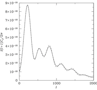
Figure 2.2: The angular power spectrum of CMB anisotropies for a spatially uniform ϕ = 0.03 (dotted),ϕ= 0 (solid), andϕ=₋0.03 (dashed).

because we are primarily concerned with the αdependence of the visibility function at very high

redshift where the simple calculation accurately captures the physics. Also, it was determined in

Ref. [2·28] that other effects, such as modifications to the details of helium recombination, or the

cooling of baryons, are small compared to the effect of variations ofαon hydrogen recombination.

In this chapter we work within the flat geometry ΛCDM cosmology with baryon and matter

densities Ωb= 0.05 and Ωm= 0.30, Hubble parameterh= 0.72, and spectral indexn= 1. Fig. 2.1 shows the visibility function g(η) = exp(₋τ)dτ /dη plotted versus the conformal time η = Rdt/a

for three different values ofϕ = (α₋α0)/α0 where α0 = 0.00729735 '1/137 is the value of the

electromagnetic fine structure parameter [2_·36]. For positive values of ϕ the visibility function is

narrower and peaks earlier, while for negative values of ϕ the visibility function is broader and

peaks later. These effects impact directly the CMB angular power spectrum because the peak of the

visibility function determines the physical distance to the last scattering surface, while the width of

the visibility function determines the thickness of the last scattering surface.

Fig. 4.13 shows the angular power spectrum of CMB anisotropies calculated assuming a spatially

(29)

For positiveϕ the angular-diameter distance is larger, so the features are scaled systematically to

higher values of l. The last-scattering surface is also narrower so that small-scale (high-l) features

are less damped due to photon diffusion. For negative ϕthe opposite holds, the smaller

angular-diameter distance scales features to lower values of lwhile the broader last-scattering surface leads

to more damping of power on small scales. In the next two Sections we derive the changes in the

angular power spectrum due to spatial fluctuations in ϕ between causally disconnected regions of

the Universe.

2.3

Power Spectra

2.3.1

CMB Power Spectra Fundamentals

The CMB radiation is observed to be a nearly isotropic background of blackbody radiation at a

temperature of TCMB= 2.728±0.004 K [2·37]. Anisotropies in the temperature are observed with

a fractional amplitude of _∼ 10−5 _[2

·38], and in the polarization with a fractional amplitude of

∼10−6 _[2

·39]. For a review of the physics of CMB anisotropies see, e.g., Ref. [2_·40].

The fundamental CMB anisotropy observables are the Stokes parameters (Θ, Q, U, V), which can

be expressed in the Pauli basis as (see, for example, Ref. [2_·41])

P(ˆn) = Θ(ˆn)1+Q(ˆn)σ3+U(ˆn)σ1+V(ˆn)σ2. (2.20)

In this expression,

Θ(ˆn) =T(ˆn)−TCMB

TCMB , (2.21)

denotes the fractional temperature anisotropy in a direction ˆn, and the remaining Stokes parameters are normalized to this quantity. HereQandU describe independent linear polarization states, while

V describes circular polarization. Because circular polarization cannot be generated via Thomson

scattering,V = 0 for the CMB.

It is convenient to introduce the quantities,

±A(ˆn) =Q(ˆn)±iU(ˆn), (2.22)

which have the spin-2 transformation properties,

±A(ˆn)→e∓2iφ±A(ˆn), (2.23)

(30)

We can expand Θ(ˆn) and±A(ˆn) in normal modes as [2·42],

Θ(ˆn) =

∞

X

l=1 m=l_X

m=−l (−i)l

r

4π

2l+ 1ΘlmY m

l (ˆn), (2.24)

and

±A(ˆn) = ∞

X

l=1 m=l

X

m=−l (₋i)l

r

4π

2l+ 1(±Alm) (±2Y m

l (ˆn)), (2.25)

where

Θlm=

Z _d3_k (2π)3Θ

(m) l (k)ei

k_·x

, (2.26)

and

±Alm=

Z d3k

(2π)3

±A(m)_l (k)

eik·x. (2.27)

HeresYml are the spin-sweighted spherical harmonics [2·43], with Ylm=0Yml , andX (m)

l (k) is the contribution to the angular modeXlmfrom wave vectors of the primordial density field of magnitude

k.

It is conventional to write the polarization in terms of the moments of the curl-free (scalar)

configurations Elm, and the moments of the divergence-free (pseudo-scalar) configurations Blm, where

±Alm=Elm±iBlm. (2.28)

We can then provide a complete description of an arbitrary CMB anisotropy field using the moments

Θlm,Elm, andBlm.

The basic observables of the random fields X(ˆn) are the power spectraCXX˜

l , defined by,

hXlm∗ Xel0_m0i=δ_ll0δ_mm0CX

˜ X

l , (2.29)

whereX,Xe _{∈ {}Θ, E, B_}and the angle brackets denote an average over all realizations. Here,

ClXX˜ = 2

π(2l+ 1)2

Z _dk

k

2

X

m=−2

k3X_l(m)∗(k)Xe_l(m)(k). (2.30)

A set of Gaussian random fields—and we expect _{Θ, E, B_} to be Gaussian—are completely

characterized by their power spectra and cross-power spectra. Because the pseudo-scalar B has

opposite parity to the scalars Θ andE, the only non-vanishing power spectra areCΘΘ

l ,ClΘE,ClEE, andCBB

l .

For small patches of sky it is an excellent approximation to treat the sky as flat and expand the

(31)

have (for example, Ref. [2·44])

Θ(ˆn) =

Z _d2_l (2π)2Θ(l)e

il_·nˆ

, (2.31)

±A(ˆn) =−

Z _d2_l

(2π)2±A(l)e

±2i(φl−φ)_eil·nˆ_, _(2.32)

and we again defineE andB through

±A(l) =E(l)±iB(l). (2.33)

In this notation the power spectra are defined by

hX(l)Xe(l0)_i= (2π)2δ2(l+l0)ClXX˜. (2.34)

Unless otherwise noted, we work within this flat-sky approximation for the remainder of the chapter.

2.3.2

Derivative Power Spectra

How do the expressions for the power spectra change if we allow for spatial fluctuations ofα? As a

warmup we first consider a spatially uniform variation,α=α0(1 +ϕ), whereϕ1.

For a given primordial density field δ(x), the temperature and polarization patterns, Θ( ˆn) and

±A(ˆn), can be calculated by solving the combined Einstein equations and radiative-transfer

equa-tions, as well as the equations for the recombination history. As discussed above, this recombination

history depends on α. Thus, the temperature and polarization fields are implicitly functions of

ϕ= (α−α0)/α0. We can expand Θ(ˆn) = Θ(ˆn;ϕ) and ±A(ˆn) = ±A(ˆn;ϕ) in Taylor series about

ϕ= 0,

Θ(ˆn) = Θ0(ˆn) +∂ϕΘ0(ˆn)ϕ+ 1 2∂

2

ϕΘ0(ˆn)ϕ2+· · ·, (2.35)

±A(ˆn) =±A0(ˆn) +∂ϕ(±A0(ˆn))ϕ+ 1 2∂

2

ϕ(±A0(ˆn))ϕ 2

· · ·. (2.36)

Inverting Eqs. (2.31) and (2.32), we find that

Θ(l) =

Z

d2nˆΘ(ˆn)e−il·ˆn

(32)

and

±A(l) =−

Z

d2nˆ(±A(ˆn))e±2i(φ−φl)e−il·nˆ. (2.38)

Thus, theϕexpansions can be written inlspace as

Θ(l) = Θ0(l) +∂ϕΘ0(l)ϕ+ 1 2∂

2

ϕΘ0(l)ϕ2+· · · , (2.39)

±A(l) =±A0(l) +∂ϕ(±A0(l))ϕ+ 1 2∂

2

ϕ(±A0(l))ϕ2+· · · , (2.40) and in fact for any fieldX ∈ {Θ, E, B}we may write

X(l) =X0(l) +∂ϕX0(l)ϕ+1 2∂

2

ϕX0(l)ϕ2+· · · . (2.41)

ToO(ϕ2_{) we then have,}

hX(l)Xe(l0)i=hX0(l)Xe0(l0)i+hX0(l)∂ϕXe0(l0)iϕ+h∂ϕX0(l)Xe0(l0)iϕ +1

2hX0(l)∂ 2

ϕXe0(l0)iϕ2+ 1 2h∂

2

ϕX0(l)Xe0(l0)iϕ2+h∂ϕX0(l)∂ϕXe0(l0)iϕ2, (2.42)

and in terms of power spectra this becomes

ClXX˜ =CX0 ˜ X0

l +

CX0∂X˜0

l +C

∂X0X˜0

l ϕ+ 1 2C

X0∂2X˜0

l +

1 2C

∂2_X 0X˜0

l +C

∂X0∂X˜0

l

ϕ2. (2.43)

Since we are for the time being assuming a spatially uniform value ofϕwe may also write

ClXX˜ =CX ˜ X l

0+∂ϕC XX˜ l

0ϕ+ 1 2 ∂

2 ϕCX

˜ X l 0ϕ

2_. _(2.44)

This allows us to make the identifications

ClXX˜

0=C X0X˜0

l ,

∂ϕCX ˜ X l

0=C X0∂X˜0

l +C

∂X0X˜0

l ,

∂ϕ2CX ˜ X l

0=C X0∂2X˜0

l +C

∂2_X 0X˜0

l + 2C

∂X0∂X˜0

l . (2.45)

These identifications make it clear how to calculate the individual ‘derivative’ power spectra. We

just differentiate Eq. (2.30) with respect to ϕ, evaluate the expression atϕ = 0, and pick off the

(33)

[image:33.612.163.481.251.543.2]

Figure 2.3: TheC∂Θ0∂Θ0

l (solid) andC Θ0∂2Θ0

(34)

[image:34.612.163.479.256.544.2]

Figure 2.4: TheC∂E0∂E0

l (solid) andC E0∂2E0

(35)

[image:35.612.164.475.254.544.2]

Figure 2.5: TheC∂Θ0∂E0

l (solid),C Θ0∂2E0

l (dashed) andC E0∂2Θ0

(36)

For example,

C∂X0∂X˜0

l =

2

π(2l+ 1)2

Z _dk

k

2

X

m=−2

k3∂ϕXl(m)∗(k)∂ϕXel(m)(k)

ϕ=0

, (2.46)

where factors like∂ϕXel(m)(k) can be calculated numerically or directly from first principles using the expressions for theXel(m)(k) derived in, for instance, Ref. [2·45]. Because they are used in subsequent calculations, we have created a modified version of the codeCMBFAST_[2_·_{46] that can compute these}

derivative power spectra. (See Figs. 2.3–2.5).

2.4

Spatial Variations of

α

We now consider the effects of spatial variations ofα(parametrized byϕ) between different causally

disconnected regions of the Universe.

First, suppose that there wereno density fluctuations, but spatial variations ofα. In that case,

photons from different points on the sky would be scattered last at different cosmological times, but

they would all still have the same frequency when observed by us. However, if there are density

fluctuations, the manner in which they are imprinted on the CMB depends on the value of α, as

discussed above. Thus, if there are spatial variations inα, the power spectra (or two-point correlation

functions) will vary from one place on the sky to another. This implies that the stochasticity of

the spatial variations inαinduce non-Gaussianity in the CMB quantified by non-zero (connected)

higher order correlation functions (trispectra and perhaps bispectra). It also implies a correction

to the mean power spectrum (i.e., that measured by mapping regions of the sky that contain many

coherence regions ofα), as well as the introduction of a non-zero curl in the polarization. All of these

effects are analogous to similar effects induced by weak lensing of the CMB. The only difference is

that in our case, the temperature and polarization patterns are modulated by a variableα, rather

than lensing by an intervening density field along the line of sight.

In this section, we first calculate the modified power spectra CΘΘ

l , ClΘE, ClEE, and ClBB. We then determine the form of the higher order correlations (bispectra and trispectra) in the next two

sections.

2.4.1

Observable Modes in the Presence of

ϕ

Fluctuations

We assume that at a given position ˆn at the surface of last scatter, the value of α is α(ˆn) =

α0[1 +ϕ(ˆn)]. Here we treat ϕ(ˆn) as a random field with angular power spectrum hϕ(l)ϕ(l0)i = (2π)2_δ2₍_l₊_l0₎_Cϕϕ

l in the flat-sky approximation.

(37)

ϕ, and that in a given directionαis constant throughout recombination. We also assume that the

dynamics responsible for the variations ofϕhave a negligible effect on the perturbation evolution,

so that the sole effect of variations ofϕare a modification of the microphysics. We will discuss the

validity of these assumptions later.

Again we expand our fields Θ(ˆn) = Θ(ˆn;ϕ) and ±A(ˆn) = ±A(ˆn;ϕ) in a Taylor series about

ϕ= 0 as

Θ(ˆn) = Θ0(ˆn) +∂ϕΘ0(ˆn)ϕ(ˆn) + 1 2∂

2

ϕΘ0(ˆn)ϕ2(ˆn), (2.47)

±A(ˆn) =±A0(ˆn) +∂ϕ(±A0(ˆn))ϕ(ˆn) + 1 2∂

2

ϕ(±A0(ˆn))ϕ2(ˆn), (2.48)

whereϕ(ˆn) is now a function of position.

By taking the Fourier transform of Θ(ˆn) we find

Θ(l) = Θ0(l) + [(∂ϕΘ0)?ϕ] (l) + 1 2

(∂ϕ2Θ0)?ϕ?ϕ

(l), (2.49)

where

[X?ψ] (l) =

Z _d2_l0

(2π)2X(l

0₎_ψ₍_l

−l0) (2.50)

is the convolution of two fieldsX andψ, and

[X?ψ?λ] (l) =

Z _d2_l0

(2π)2[X?ψ] (l

0₎_λ₍_l

−l0), (2.51)

is the double convolution of three fieldsX,ψ, andλ.

Similarly, taking linear combinations of the Fourier transforms of±A(ˆn) we find that

E(l) =E0(l) + [(∂ϕE0)?cϕ] (l)−[(∂ϕB0)?sϕ] (l) +1

2

(∂2

ϕE0)?cϕ?ϕ

(l)₋1 2

(∂2

ϕB0)?sϕ?ϕ

(l), (2.52)

and

B(l) =B0(l) + [(∂ϕB0)?cϕ] (l) + [(∂_ϕE₀)?sϕ] (l) +1

2

(∂ϕ2B0)?cϕ?ϕ

(l) +1 2

(∂ϕ2E0)?sϕ?ϕ

(l), (2.53)

where

[X?cψ] (l) =

Z _d2_l0

(2π)2cos (2φl0)X(l

0₎_ψ₍_l

(38)

and

[X?sψ] (l) =

Z _d2_l0

(2π)2sin (2φl0)X(l

0₎_ψ₍_l

−l0), (2.55)

are the even- and odd-parity spin-2 weighted convolutions ofX andψrespectively.

Examining these expressions we find that a given mode X(l) receives corrections due to the combination of modes _{∂n

ϕX0(l0), ϕ(l1), ϕ(l2), . . . , ϕ(ln)} such that Pni=0li = l. Furthermore, the

E and B modes mix so that, for example, the modeB(l) can be induced by the combinations of modes _{∂n

ϕE0(l0), ϕ(l1), ϕ(l2), . . . , ϕ(ln)}such that Pni=0li = l. These effects modify the angular power spectra of CMB anisotropies, and introduce higher-order connected (non-Gaussian) correlation

functions.

2.4.2

The

ΘΘ

Power Spectrum

Using Eq. (2.49) we find that the expansion for the two point correlation function (in Fourier space)

is

hΘ(l)Θ(l0)_i=_hΘ0(l)Θ0(l0)i+hΘ0(l) [∂ϕΘ0?ϕ] (l0)i+h[∂ϕΘ0?ϕ] (l)Θ0(l0)i +1

2hΘ0(l)

∂ϕ2Θ0?ϕ?ϕ

(l0)_i+1 2h

∂ϕ2Θ0?ϕ?ϕ

(l)Θ0(l0)i+h[∂ϕΘ0?ϕ] (l) [∂ϕΘ0?ϕ] (l0)i (2.56)

to O(ϕ2_{). In the above expression and what follows we adopt the convention that the differential}

operators∂ϕ act only the the field immediately following them.

We assume that Θ0andϕare zero-mean Gaussian random fields without higher-order connected

correlators. By writing out the convolutions and Wick expanding the correlators it is easy to verify

that correlators involving an odd number of fields vanish, and so there are no corrections to first

order inϕ. It is also straightforward to verify that

hΘ0(l)[∂ϕ2Θ0?ϕ?ϕ](l0)i=h[∂ϕ2Θ0?ϕ?ϕ](l)Θ0(l0)i = (2π)2_δ2₍_l₊_l0₎h_σ(ϕϕ)_CΘ0∂2Θ0

l + 2σ(ϕ∂

2_Θ 0)_CΘ0ϕ

l

i

, (2.57)

where

σ(ψλ)=

Z _d2_l (2π)2C

ψλ

l (2.58)

is the covariance between two fieldsψandλ. Similarly we can show that

h[∂ϕΘ0?ϕ] (l) [∂ϕΘ0?ϕ] (l0)i= (2π)2δ2(l+l0){Cϕϕ?C∂Θ0∂Θ0_l+C∂Θ0ϕ?C∂Θ0ϕ_l}, (2.59)

(39)

[image:39.612.164.480.101.394.2]

Figure 2.6: The solid curve shows the ΘΘ power spectrum for the Gaussian correlation function for

ϕwith angular correlation scaleθc= 1◦and varianceσ(ϕϕ)= 9×10−4(fluctuations inϕat the 3% level). The dashed curve shows the power spectrum without fluctuations inϕ.

Collecting all terms we find that to leading order the average power spectrum including

fluctua-tions inϕis

ClΘΘ=ClΘ0Θ0+σ

(ϕϕ)_CΘ0∂2Θ0

l + 2σ

(ϕ∂2_Θ 0)_CΘ0ϕ

l +

Cϕϕ?C∂Θ0∂Θ0

l+

C∂Θ0ϕ_?C∂Θ0ϕ

l. (2.60)

Note that the corrections to CΘ0Θ0

l involve couplings between the derivative power spectra, which are calculated as described in Section 2.3.2, andC_lϕϕand the various cross power spectra, which are specified by the model that generates spatial variations inϕ.

In general Θ0andϕmay be correlated if, for instance, they are generated by a common

mecha-nism or if they are strongly coupled through evolution equations. We discuss in Section 2.7 why we

do not expect the latter source of correlations to be important as long as the energy in theϕfield

(40)

case where Θ0andϕhave no cross-correlation, the expression simplifies to

ClΘΘ=ClΘ0Θ0+σ

(ϕϕ)_CΘ0∂2Θ0

l +

Cϕϕ?C∂Θ0∂Θ0

l. (2.61)

The result for CΘΘ

l will of course depend onC ϕϕ

l . To illustrate we consider a simple model in whichϕis highly correlated on angular scales smaller than the correlation angleθc, and uncorrelated on larger scales. (Below we discuss a physical model that may produce such a correlation function).

We thus have,

hϕ(0)ϕ(θ)_i=σ(ϕϕ)e−(θ/θc)2_. _(2.62)

In the flat-sky approximation we have

C_lϕϕ=

Z

d2θhϕ(0)ϕ(θ)ie−il·θ

, (2.63)

which implies that

C_lϕϕ=πθc2σ(ϕϕ)e−

1 4l

2_θ2

c_. _(2.64)

In this case the average ΘΘ power spectrum is

ClΘΘ=C Θ0Θ0

l +σ(ϕϕ)

h

CΘ0∂2Θ0

l +

θ2 c 2

Z

dl0l0e−14(l 2_+l02

)θ2 c_I 0 _θ2 c 2ll 0

C∂Θ0∂Θ0

l0 i

, (2.65)

where In is the nth-order modified Bessel function of the first kind. We show this average power spectrum in Fig. 2.6. The main effect of ϕ fluctuations is to reduce the amplitude of oscillatory

features in the damping tail. This effect can be understood by noting that patches o