Forces, Stresses, and the (Thermo?) Dynamics of Active Matter: The Swim Pressure

(1)

Matter: The Swim Pressure

Thesis by

Sho C Takatori

In Partial Fulfillment of the Requirements for the degree of

Doctor of Philosophy

CALIFORNIA INSTITUTE OF TECHNOLOGY Pasadena, California

2017

(2)

c 2017

Sho C Takatori

ORCID: 0000-0002-7839-3399

(3)

ACKNOWLEDGEMENTS

I would like to express my sincere gratitude for the support of many amazing people during my PhD studies at Caltech. First, I would like to thank my thesis advisor, John Brady. Aside from his exceptional scientific guidance and his remarkable ability to know the answer to a problem before actually solving it, the quality I appreciate most about Professor Brady’s advising is his deep respect and trust for my independence. When I declared one day, “I will pursue experiments” (in an all-theory and simulation group), he allowed me to conduct experiments across three different research groups at Caltech and at ETH Zürich. When I incorporated Disney hats and references into conference presentations, he suggested that I go pursue ‘experiments’ at Disneyland. I am very fortunate to have learned from a world-class researcher; his academic curiosity, integrity, and rigor have set a high standard that I will continuously aim for as I begin my academic career.

I would like to thank the members of my thesis committee – Zhen-Gang Wang, Rob Phillips, and Mikhail Shapiro. Professor Phillips and Professor Shapiro have gen-erously allowed me to use their lab resources to pursue my experimental studies, which would not have been possible without their support. I would like to thank Dr. Heun-Jin Lee in Professor Phillips’ group for teaching me various techniques of ex-perimental biophysics and microscopy. His extensive knowledge in the biophysical behavior of cells have sparked my curiosity in a variety of fields.

I would like to express my great gratitude for Professor Jan Vermant and Dr. Raf De Dier at ETH Zürich, who had the heroic patience and dedication to teach a theorist with an∼ O() knowledge of basic wet lab techniques how to conduct experiments in soft matter. Raf was the best sensei I could have wished for.

(4)

Words cannot express how much I have been supported by the love and support from friends and family outside of Caltech. My parents have made tremendous sacrifices throughout my life, just to help me be the best and happiest I could be, and I strive to do the same for them in the coming years. I would like to express my heartfelt gratitude to Gigi for always putting a smile on my face and being willing to lend a sympathetic ear. My life would not be the same without her optimism, sense of humor, and ever-enduring kindness. Thank you to Kevin for a continuous source of the best, funniest, and most legendary stories and adventures. Finally, I thank my sister and gastroenterologist, Dr. Takatori, for her unwavering support and love. I cannot be more proud of having a sister who saves the lives of patients suffering from hideous diseases like Inflammatory Bowel Disease.

(5)

ABSTRACT

A core feature of many living systems is their ability to move, self-propel, and be active. From bird flocks to bacteria swarms, to even cytoskeletal networks, ac-tive matter systems exhibit collecac-tive and emergent dynamics owing to their con-stituents’ ability to convert chemical fuel into mechanical activity. Active matter systems generate their own internal stress, which drives them far from equilibrium and thus frees them from conventional thermodynamic constraints, and by so doing they can control and direct their own behavior and that of their surrounding environ-ment. This gives rise to fascinating behaviors such as spontaneous self-assembly and pattern formation, but also makes the theoretical understanding of their com-plex dynamical behaviors a challenging problem in the statistical physics of soft matter.

(6)

PUBLISHED CONTENT AND CONTRIBUTIONS

[1] S. C. Takatori, W. Yan, and J. F. Brady. “Swim pressure: stress generation in active matter”. Phys Rev Lett 113.2 (2014), p. 028103. doi: 10 . 1103 / PhysRevLett.113.028103.

S.C.T. participated in the conception of the project, conducted simulations, analyzed the data, and participated in the writing of the manuscript.

[2] S. C. Takatori and J. F. Brady. “Swim stress, motion, and deformation of active matter: effect of an external field”.Soft Matter10.47 (2014), pp. 9433– 9445.doi:10.1039/C4SM01409J.

[3] S. C. Takatori and J. F. Brady. “Towards a thermodynamics of active matter”. Phys Rev E 91.3 (2015), p. 032117.doi:10.1103/PhysRevE.91.032117.

[4] S. C. Takatori and J. F. Brady. “A theory for the phase behavior of mixtures of active particles”.Soft Matter11.40 (2015), pp. 7920–7931.doi:10.1039/ C5SM01792K.

[5] S. C. Takatori and J. F. Brady. “Forces, stresses and the (thermo?) dynamics of active matter”.Curr Opin Colloid Interface Sci21 (2016), pp. 24–33.doi: 10.1016/j.cocis.2015.12.003.

[6] S. C. Takatori*, R. De Dier*, J. Vermant, and J. F. Brady. “Acoustic trapping of active matter”.Nat Commun7 (2016).doi:10.1038/ncomms10694.

S.C.T. participated in the conception of the project, participated in the devel-opment of the experiments and simulations, analyzed the data, and partici-pated in the writing of the manuscript. (* equal contribution).

[7] S. C. Takatori and J. F. Brady. “Superfluid behavior of active suspensions from diffusive stretching”. Phys Rev Lett118.1 (2017), p. 018003.doi:10. 1103/PhysRevLett.118.018003.

(7)

LIST OF ILLUSTRATIONS

Number Page

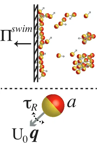
1.1 Self-propelled bodies exert a unique mechanical ‘swim pressure’ (Takatori, Yan, and Brady, Phys Rev Lett, 2014), Πswim, on an os-motic boundary owing to their self-motion. In a simple model of active matter, particles of size atranslate with a swim velocityU0q and reorient with a reorientation time scaleτR, where the unit

orien-tation vectorqindicates the direction of swimming. . . 3 1.2 Dependence of swimmer concentration on (A) swim pressure and

(B) interparticle (collisional) pressure scaled with the swim activity ksTs ≡ ζU₀2τR/6. Data are from Brownian dynamics simulations,

where the reorientation Péclet number PeR ≡ a/(U0τR) is the

ra-tio of the swimmer size to its run length. In (A), for large PeR the

data collapse on the solid line representing a linear increase of the active pressure with concentration,Πswim = nksTs. As PeR → 0 the

swim pressure decreases with increasing concentration and agrees withΠswim = nksTs(1−φ−φ2) (dashed curve) (Takatori and Brady,

Phys Rev E, 2015). In (B), the collisional pressure increases mono-tonically with concentration for all PeR. . . 16

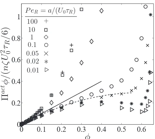
1.3 Nonequilibrium Πact-φ phase diagram, where Πact = Πswim + ΠP and is scaled with the swim activity ksTs ≡ ζU₀2τR/6. Data are

from Brownian dynamics simulations, where the reorientation Pé-clet number PeR ≡ a/(U0τR) is the ratio of the swimmer size to its

run length. The solid line represents a linear increase of the active pressure with concentration, Πact =nksTs. The dashed blue curve is

the Carnahan-Starling equation of state for Brownian hard-spheres. ForPeR < 1/3 we observe a negative ‘second virial coefficient,’ and

for PeR . 0.03 a non-monotonic pressure variation (analogous to a

(10)

1.4 Phase diagram in the PeR − φplane for a 3D active system.

Color-bar represents the magnitude of the active pressure scaled with the swim activity ksTs ≡ ζU₀2τR/6, and the blue and red curves are the

binodal and spinodal, respectively. The critical point is shown with a red star. The open and filled symbols are simulation data (Wysocki, Winkler, and Gompper, Europhys Lett, 2014) with a homogeneous and phased-separated state, respectively. . . 19 2.1 The swim, Πswim, and Brownian, ΠB, pressures computed using

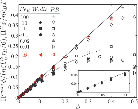
bounding walls (“Walls”) and from Eq 2.1 without walls (periodic boundaries, “PB”) for variousPeR = a/(U0τR). The solid black line

corresponds to a linear increase of pressure withφ. The dashed curve is the dilute theory expression (Eq 2.3). The inset is a magnification of the swim pressure at diluteφforPeR ≤ 1. . . 35

2.2 Nonequilibrium Πact-φ phase diagram, where Πact = Πswim+ ΠP. The data are from BD simulations (with periodic boundaries) and the dashed curve is the analytical theory, Eq 2.4, withPeR =a/(U0τR) =

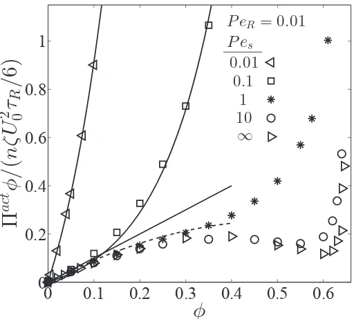
0.05. . . 38 2.3 Effect of translational Brownian motion on the Πact-φ phase

dia-gram, whereΠact =Πswim+ΠP+ΠB. The data are BD simulations for various Pes = U0a/D0 with fixed PeR = a/(U0τR) = 0.01.

The solid curves are theoretical expressions of osmotic pressures of Brownian particles. The dashed curve is the analytical theory, Eq 2.4. 39 3.1 Active Janus particles in a weak acoustic trap. (a-c) Snapshots of

(11)

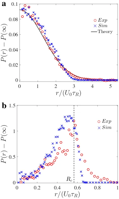
3.2 Probability distribution of confined active Janus particles. (a) 2µm

swimmers with α ≡ kτR/ζ = 0.29 follow a Boltzmann distribution

(solid black curve is the analytical theory, Eq 3.1). (b) Distribution of 3µm swimmers withα = 1.76 has a peak near Rc = ζU0/k

(ver-tical dashed black line) and decreases to zero for r > Rc. In both

(a,b), the red and blue symbols are data from experiment and Brow-nian dynamics simulations, respectively. Data are averages of mea-surements of over 500 snapshots for a duration of 50s, each frame consisting ≈ 100 and 20 particles for the α = 0.29 and α = 1.76 cases, respectively. . . 47 3.3 ‘Explosion’ of active crystal. Explosion of swimmer-crystal in (a

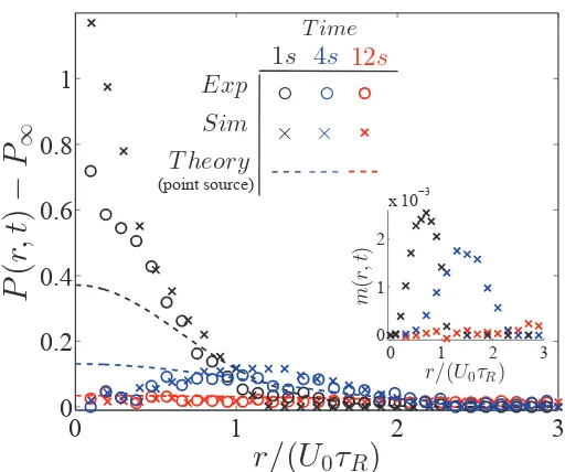
-d) experiments and (e-h) Brownian dynamics simulations. (a,e) A strong trapping force draws the swimmers into a dense close-packed 2D crystal. (b,f) A subsequent release of the trap frees the swim-mers, causing the crystal to explode. (c,g) At later times, a ballistic shock propagates outward like a traveling wave. (d,h) At long times, the swimmers spread diffusively. . . 48 3.4 Evolution of active-crystal ‘explosion.’ Transient probability density

(12)

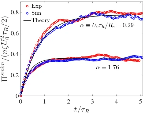
3.5 Swim pressure of Janus particles in different degrees of confinement. The parameter α ≡U0τR/Rcis a ratio of the particles’ run length to

the trap size Rc = ζU0/k. The solid black curves are the theoretical

prediction with a harmonic trap approximation, and the red and blue symbols are results from experiments and Brownian dynamics sim-ulations, respectively. A smaller trap size diminishes the distance the particles travel between reorientations and decreases the swim pressure. The experimental and simulation data are averages of 150 and 90 independent particle trajectories for a duration of 40sfor the α=0.29 andα =1.76 cases, respectively. . . 54 4.1 Phase diagram in the PeR −φplane in (A) 3D and (B) 2D. The

col-orbar shows the active pressure scaled with the swim energy ksTs =

ζU2

0τR/6, and the blue and red curves are the binodal and spinodal, respectively. The critical point is shown with a red star. The open and filled symbols are simulation data with a homogeneous and phased-separated state, respectively. . . 65 4.2 Nonequilibrium chemical potential as a function of Πact for PeR =

a/(U0τR) = ζU0a/(6ksTs) = 0.02, where ksTs = ζU₀2τR/6 is the

swimmers’ energy scale. The symbols are BD simulations (Takatori, Yan, and Brady,Phys Rev Lett, 2014) and the curve is the model, Eq 4.2. . . 67 4.3 Gibbs free energy (FE) as a function ofφfor fixed values ofPeRand

Πactφ/(nksTs) = 0.18, where ksTs = ζU₀2τR/6. The red and blue

curves are the spinodal and binodal, respectively. The black arrow points towards decreasing PeR at fixedΠact. The filled color circles

denote the stable states. . . 69 5.1 Schematic of the mixing process of purely Brownian suspensions

(top) and active systems (bottom) that are initially at two different “temperatures.” The Brownian particles thermally equilibrate their thermal energy kBT whereas the active swimmers do not share their

(13)

5.2 Long-time self diffusivity of a passive particle as a function of the total area fraction for different values of the active swimmer frac-tion xa. The known Brownian diffusivity D0 was subtracted from

the results. The solid line is the analytical theory and symbols are Brownian dynamics (BD) simulations. All data collapse onto a sin-gle curve when the diffusivity is scaled withU0axa/2. . . 84

5.3 Swim pressure exerted by active swimmers in a mixture as a function of the total area fraction φ = φa+ φd for different values of active

compositionxa =φa/φand fixedPeR ≡ a/(U0τR)= 0.1. Subscripts

“a” and “d” refer to active and passive particles, respectively. The solid curve is the mechanical theory Eq 5.2 and the symbols are BD simulations. The swimmer activityksTs ≡ ζU₀2τR/2. . . 88

5.4 Collisional pressure exerted by active and passive particles ΠP =

Π_aP+ΠP_d for fixedPeR ≡ a/(U0τR) = 0.1 as a function of the total

area fraction φ= φa+φd and different values of active composition

xa= φa/φ. The solid curve is the mechanical theory Eq 5.5 plus Eq

5.6 for xa = 0.3, and the symbols are BD simulations. We take the

swimmer reorientation to be thermally induced so thatkBT/(ksTs) =

8Pe2_R/3. . . 89 5.5 Phase diagram in thePeR−φplane in 2D for a fixed active swimmer

compositionxa =0.5. The colorbar shows the active pressure scaled

with the swim activityksTs = ζU₀2τR/2. The open and filled symbols

(14)

5.6 Phase diagram in thePeR−φplane in 2D for different active

swim-mer compositions xa = φa/φ. The solid curves are the spinodals

delineating the regions of stability based upon fluctuations in the total particle density. The two-phase region diminishes as xa

de-creases. Steady-state images from BD simulations are shown for PeR = 0.01,xa = 0.05 atφ = 0.35 (left) andφ = 0.6 (right),

corre-sponding to a homogeneous and phased-separated state, respectively. The red and white circles are the active and passive particles, respec-tively. . . 93 6.1 Schematic of the shape, size, and motion of a soft, compressible gel

loaded with light-activated synthetic colloidal particles. When both the light and external field (H) are turned on, the gel translates in the direction of the field (shown by arrows on the gel). The external field strength can be tuned to change the shape, size, and velocity of the gel.108 6.2 Schematic of the motion of a soft, compressible gel loaded with

ac-tive particles when the external field is rotated by 90 degrees. The shape and trajectory of the gel depends on the relative rate of rotation of the field and the strength of the field. . . 111 6.3 Definition sketch of an active particle at position z with orientation

q in an external field,H. . . 114

6.4 Average translational velocity along the external field as a function of χR. The solid curve is the exact analytical solution, and the circles

are data from Brownian dynamics (BD) simulations. . . 120 6.5 The swim stress in the parallel (in black) and perpendicular (in red)

directions as a function of χR, computed in the simulations from

σswim ₌ _−nhx0_Fswim0_i_{(in circles) and also from first obtaining the}

effective translational diffusivity and then usingσswim = −nζhDswimi (in squares). The solid and dashed curves are the exact and asymp-totic analytical solutions, respectively. . . 121 6.6 The first normal swim-stress difference, N1 = σskwim −σ

swim

⊥ , as a function of χR. The circles are results from BD simulations, and the

(15)

6.7 The swim pressure, Πswim = −trσswim/3, as a function of χR. The

circles are results from BD simulations, and the solid and dashed curves are the exact and asymptotic analytical solutions, respectively. The illustration shows an instantaneous configuration of the swim-mers under a weak (sketch on left) and moderate (on right) external field. . . 123 6.8 (A.) Swim stress in the parallel (in black) and perpendicular (in red)

directions as a function of χR for αH0 = 1. TheαH0 parameter al-lows the swimming speed to vary with particle orientation. (B.) First normal swim-stress difference. The illustration shows an instanta-neous configuration of the swimmers under a weak (sketch on left) and moderate (on right) external field. In both (A) and (B), the solid curves are the exact solutions, and the dashed curves are the asymp-totic solutions. In (A) BD simulation results are shown in circles and squares for the parallel and perpendicular directions, respectively. . . 126 6.9 The swim pressure, Πswim = −trσswim/3, as a function of χR for

αH0= 1. The circles are results from BD simulations, and the solid and dashed curves are the exact and asymptotic analytical solutions, respectively. The illustration shows an instantaneous configuration of the swimmers under a weak (sketch on left) and moderate (on right) external field. . . 128 7.1 Schematic of active particles with swimming speedU0and

reorien-tation time τR in simple shear flow with fluid velocity u∞x = γ˙y,

where ˙γ is the magnitude of shear rate. The unit vector q(t) spec-ifies the particle’s direction of self-propulsion. Diffusion of active particles along the extensional axis of shear acts to ‘stretch’ the fluid and reduce the effective shear viscosity, similar to the effect that the hydrodynamic stress plays for pusher-type microorganisms. . . 137 7.2 Swim diffusivity as a function of shear Péclet number for two diff

(16)

7.3 Comparison of our model, Eq 7.4, with shear experiments of López et al (López, Gachelin, Douarche, Auradou, and Clément,Phys Rev Lett, 2015) with motile E. coli bacteria at different concentrations. Horizontal dashed lines for small Peare the analytical solutions of Eq 7.6. . . 143 7.4 Effective suspension viscosity of spherical active particles at dilute

concentrations and reorientation Péclet number PeR ≡ a/(U0τR) =

0.035. Filled circles and crosses at large Peare experimental data of Rafaï et al (Rafaï, Jibuti, and Peyla, Phys Rev Lett, 2010) using ‘puller’ microalgae C. Reinhardtii. The solid curve is the analytical theory of Eq 7.5, and the open circles are BD simulation results. In-set: Magnification at largePeto show agreement with experiments. 144 8.1 Swim and Reynolds pressures of a dilute system of swimmers with

finite inertia, where Π = −trσ/3. The red (Πswim) and blue (ΠRey) curves and symbols are the analytical theory of Eqs 8.3 and 8.4 and simulation data, respectively. The solid black line is the sum of the swim and Reynolds stresses. The Brownian osmotic pressure ΠB = nkBT has been subtracted fromΠRey. . . 157

8.2 (A) Swim pressure, Πswim, and (B) Reynolds pressure, ΠRey, as a function of volume fraction of particles, φ, for different values of StR ≡ (M/ζ)/τR and a fixed reorientation Péclet number, PeR ≡

a/(U0τR) = 0.01. The symbols and solid curves are the simulation

data and analytical theory, respectively. The Brownian osmotic pres-sureΠB = nkBT has been subtracted from the Reynolds pressure. . . 160

8.3 Sum of swim and Reynolds pressures,Πswim+ΠRey = −tr(σswim+ σRey_{)/3, as a function of volume fraction of particles}_φ_{for di}_ff_erent

values of StR ≡ (M/ζ)/τR and a fixed reorientation Péclet number,

PeR ≡ a/(U0τR) = 0.01. The symbols and solid curve are the

simu-lation data and analytical theory of Eq 8.6, respectively. The Brown-ian osmotic pressure ΠB = nkBT has been subtracted from the total

pressure. . . 162 8.4 Interparticle collisional pressure, ΠP, as a function of volume

frac-tion of particles, φ, for different values of StR ≡ (M/ζ)/τR and a

fixed reorientation Péclet number, PeR ≡ a/(U0τR) = 0.01. The

(17)

C h a p t e r 1

INTRODUCTION TO THE DYNAMICS OF ACTIVE MATTER

This thesis consists of independent chapters that are presented in a form suitable for publication, with Chapters 1-7 already published. This introductory chapter provides an overview of the basic features of active matter systems and a few of the main results of the thesis. Subsequent chapters provide a more in-depth analysis of the dynamics of collective motion exhibited by active matter, as well as additional topics not covered in this introduction. I lay the groundwork in Chapter 2 for all of the work in this thesis by introducing the principle of a unique mechanical swim pressure exerted by active matter systems. I present in Chapter 3 an experimen-tal measurement of the swim pressure by employing the novel use of an acoustic tweezer to confine self-propelled particles in a potential well. In Chapters 4 and 5, I use the swim pressure framework to construct an equation of state of active matter and predict its self-organization and unusual phase behavior. I analyze in Chapter 6 the effect of an external orienting field on the dynamics of self-propelled bodies, and provide potential applications of active matter for nano/micromechanical devices and motors with tunable material properties. In Chapter 7, I discover that active self-propulsion engenders an additional contribution to the suspension shear stress, and explain why and how fluids containing motile bacteria can exhibit superfluid-like behaviors with zero effective shear viscosity. Lastly, I analyze in Chapter 8 the effects of finite particle inertia on the stress generation of active matter to extend the swim pressure framework to larger swimmers such as fish and birds.

This introductory chapter includes content from our previously published article:

[1] S. C. Takatori and J. F. Brady. “Forces, stresses and the (thermo?) dynamics of active matter”.Curr Opin Colloid Interface Sci21 (2016), pp. 24–33.doi: 10.1016/j.cocis.2015.12.003.

1.1 Introduction

(18)

be observed in equilibrium thermodynamic systems, such as spontaneous collective motion and swarming. Even minimal kinetic models of active Brownian particles exhibit self-assembly that resembles a gas-liquid phase separation from classical equilibrium systems. Self-propulsion allows active systems to generate internal stresses that enable them to control and direct their own behavior and that of their surroundings. In this introduction we discuss the forces that govern the motion of active Brownian microswimmers, the stress (or pressure) they generate, and the im-plication of these concepts on their collective behavior. We focus on recent work involving the unique ‘swim pressure’ exerted by active systems, and discuss how this perspective may be the basic underlying physical mechanism responsible for self-assembly and pattern formation in all active matter. We discuss the utility of the swim pressure concept to quantify the forces, stresses, and the (thermo?) dy-namics of active matter.

A distinguishing feature of many living organisms is their ability to move, to self-propel, to be active. Constituents of “active matter” systems are capable of in-dependent self-propulsion by converting fuel into mechanical motion, and include both microscopic entities like microorganisms and motor proteins within our cells to large bodies like fishes and birds. Inanimate, nonliving bodies can also achieve self-propulsion using mechanisms that are different than living organisms, but the outcome of their collective behavior is not necessarily different between living and nonliving active systems. Indeed, active matter systems of all scales have the tendency to associate together and move collectively, from colonies of bacteria, swarms of insects, flocks of birds, schools of fish, and herds of cattle. A question arises as to the micromechanical origin for living organisms to exhibit collective and coherent motion, and whether it can be explained and expressed using basic physical quantities.

All active matter systems are intrinsically out of equilibrium, a trait which allows self-propelled entities to display fascinating behaviors that cannot be observed in thermodynamic systems in equilibrium such as spontaneous self-assembly and pat-tern formation [1, 2, 3, 4]. At the same time, nonequilibrium systems like active matter have very complex and specialized networks relating the input to the re-sponse, and which make the theoretical understanding of their behaviors a chal-lenging and intriguing problem in soft matter and statistical mechanics.

(19)

W

swim

U

₀

q

a

[image:19.612.227.385.65.297.2]

o

R

Figure 1.1: Self-propelled bodies exert a unique mechanical ‘swim pressure’ (Taka-tori, Yan, and Brady, Phys Rev Lett, 2014), Πswim, on an osmotic boundary owing to their self-motion. In a simple model of active matter, particles of sizeatranslate with a swim velocityU0qand reorient with a reorientation time scaleτR, where the

unit orientation vectorqindicates the direction of swimming.

(20)

separation in a simple active Brownian suspension. Next, we discuss whether the notion of an effective ‘temperature’ of active matter can be used to describe the ac-tivity of an active suspension. In Sec 1.8 we explain how active systems may exert an ‘internal’ force that behaves just like an external body force like gravity and how one can describe active systems using a microscopic theory. Finally, in Sec 1.9, we conclude with suggestions for future research.

1.2 Active matter systems

Among a large class of active matter systems, we focus our attention on microscopic swimmers whose sizeaand swimming speedU0are such that the Reynolds number associated with their self-motion is negligibly smallRe ≡U0a/ν∼ O(10−6−10−2) (νis the fluid kinematic viscosity, taken to be that of water), and hence their dynam-ics are governed by the Stokes equations. Unlike large organisms like fish that self-propel by making use of inertia in the surrounding fluid, bodies at low-Reynolds number must break time-reversal symmetry to move. Active matter systems need not be living, and in fact intensive research has gone into the fabrication of nonliv-ing, synthetic microswimmers, as described below.

Inanimate, synthetic particles

(21)

gener-ate self-propulsion due to an ionic current resulting from a difference in electron affinities of the two metals. In self-diffusiophoresis [15], autonomous motion is at-tributed to the osmotic pressure gradient induced by an asymmetric distribution of solutes around the particle [16]. However, the full mechanism behind the motion of self-diffusiophoretic particles is not fully understood [17]. Nonetheless, Janus microswimmers have become a standard model for active Brownian colloids and are used frequently by researchers around the world.

Active Janus particles swim roughly at a fixed speed U0 in a direction specified by a body-fixed unit orientation vector q, as shown in Fig 1.1. The orientationq changes by Brownian motion with rotational diffusivity DR so the Janus particle

has a characteristic reorientation timescale given byτR∼ 1/DR.

Light-activated Janus particles [18, 19, 20] offer a convenient method to control the speedU0of the particles—the chemical reaction taking place at the particle surface is trigged by light, which allows researchers to instantly turn on or offthe particle motion. Researchers have also fabricated Janus motors with layers of ferromagnetic material that allow for magnetic alignment of the swimmer orientation to move in a directed fashion [21], providing a method to control the reorientation time τR in

addition to the speedU0.

Living microorganisms

In addition to artificial microswimmers, another large class of active matter include living microorganisms, which can be divided into 4 sub-categories based upon their swimming mechanism: ciliates such asParameciummobilize small flagella around their body; flagellates such as E. coli activate a single or multiple flagella; spiro-chetes such asLeptospirause axial filaments to undergo a twisting, corkscrew mo-tion; and amoebas such asAmoeba proteusdeform their entire body. Many motile microorganisms likeE. coliundergo a run-and-tumble where they alternate between a “run,” where they swim straight towards a given orientation with speedU0, and a “tumble” which aligns them into a new random direction with frequencyω [22]. Like a synthetic active Janus particle, the activity of a motile microorganism may be described by an average speedU0and reorientation timeτR ∼1/ω.

(22)

pref-erentially swimming towards (or away from) chemical gradients of nutrients (or toxins) [23]. Magnetotactic microorganisms such as Magnetospirillum have or-ganelles called magnetosomes that contain magnetic crystals that help the organism align along imposed magnetic field lines [24]. Other common examples of taxis swimmers include phototactic [25] and gravitactic [26] bacteria. Chlamydomonas reinhardtiiis a green alga that swims with a breast-stroke motion and possesses an eyespot that allows the alga to orient itself and swim toward a light source [27].

Molecular motors and active gels

Sub-cellular metabolic processes and energy-consuming enzymes like motor pro-teins are another important class of active soft matter that has been studied inten-sively and is of significant biological relevance[28, 4, 2, 29]. Molecular motors consume chemical fuel (like ATP) to generate active stresses that are responsible for cell locomotion, muscle contraction, mechanotransduction, and many other critical cellular processes. In particular, simplified model systems of filaments and motors that constitute the eukaryotic cellular cytoskeleton have led to a deeper fundamen-tal understanding of the inner workings of the cell. Hydrodynamic theories for active polar and nematic gels [30, 31, 32, 33, 34] were developed by invoking lin-ear irreversible thermodynamics [35, 36] for systems perturbed slightly away from equilibrium. The resulting theory gives a relationship between the active stress, suspension flux on a continuum level, and the chemical potential difference of ATP and its reaction products generated by the motor. By providing an extension to soft matter physics, active gels and hydrodynamic theories have successfully elucidated a variety of nonequilibrium biological phenomena, including the prediction of cell polarity and pattern formation [37, 38, 39, 40], actin cortex flows in developing embryos [41], and microtubule-based pronuclear motion [42]. Active gel theory has the potential to explain other areas of physics, including mechanical fracture, jamming, and wetting [28].

1.3 Other open driven systems

(23)

One example is driven reactive mixtures in electrochemical systems, where ex-ternally controlled chemical reactions can control the onset of phase separation [44]. Another example is the autocatalytic reactions in biochemical systems, where chemically-driven phase separations can control patterns that lead to membrane-less organelles [37, 45]. The thermodynamic stability of dissipative structures have been studied using concepts of irreversible thermodynamics and entropy generation [43]. A very interesting extension of the present swim pressure theory would be to understand how it relates to the formalism of linear irreversible thermodynamics and the associated ideas on entropy production.

Now that we have briefly reviewed the different classes of active systems within a broader class of open driven systems, in the next section we discuss the self-propulsive forces that govern their motion in the Stokes regime, explaining why and how microorganisms are able to move while being ‘force-free.’

1.4 ‘Force-free’ motion

Swimming microorganisms and inanimate self-propelled particles move in the Stokes regime and undergo so-called ‘force-free’ motion. This phrase is somewhat am-biguous, as all non-accelerating bodies are by definition force-free, i.e.,m(dU/dt)=

P

F = 0. This is true for an airplane traveling at constant speed, where its propul-sive force is balanced by the frictional forces acting against the body. The same ap-plies for microscopic bodies swimming at low-Reynolds number. What researchers actually mean when they say active matter undergoes force-free motion is that the body experiences noexternalforce causing the body to move.

What force then, if any, induces the body to swim? Suppose we have a ciliated microorganism (such asParamecium) which swims by beating many small flagella cooperatively along its body surface, such that the velocity of the surrounding fluid at any point on the swimmer surface isu(x) = U +Ω × (x − X)+us(x), where U and Ω are translational and angular velocities of the body (about its center), X is the position of the body center, x is the position along the body surface, and us(x) is the ‘slip velocity’ induced by the deformations happening along the ciliated body surface. The slip velocity can be expressed in terms of surface moments: us(x) = Es · x0+ Bs : (x0x0− I(x0)2) +· · ·, where x0 = x − X, and the surface moment tensors Es(t),Bs(t), etc are in general functions of time and set by the swimming gait.

(24)

the interactions among many swimmers. For example, the spherical squirmers of Blake [46] and Ishikawa et al [47] invoke a quadrupolar moment Bs to achieve self-propulsion. The use of Stokesian dynamics to simulate various classes of mi-croswimmers is given in Swan et al [48]. The only requirement for the slip velocity us is that it contributes no net translation or rotation to the particle (i.e., it has zero mean and zero antisymmetric first moment).

The total hydrodynamic force/torque on the swimmer can be written as

FH =−RF U· U −_{| {z }}RF E : Es −RF B Bs− · · ·

= Fdr ag + Fswim, (1.1)

where we grouped the force/torqueF = (FH,LH) and translational/angular veloc-ities U = (U,Ω), and the hydrodynamic resistance tensors RF U,RF E,RF B, etc couple the force to the velocity and to the ‘squirming set’Es(t),Bs(t), etc.

Although we motivated this discussion using a ciliated microorganism, the same development applies for self-diffusiophoretic Janus particles which also exhibit a fluid ‘slip velocity’ near the particle surface due to solvent backflow induced by the flux of chemical reactants/products along the particle surface. In fact, we can generalize this structure to all classes of microswimmers by recognizing that the resistance tensors are now functions of time, rather than being fixed for the ciliates.

Equation 1.1 has been written as a sum of the hydrodynamic drag forceFdr agand self-propulsive ‘swim force’Fswim. A microswimmer moves in the Stokes regime, so its motion is ‘force-free’: P_F = _FH ₊_Fext ₌ _{0, where}_Fext _{is any external}

force such as gravity. In the absence of an external field, Fext = 0 and we have FH =0. Using Eq 1.1, we obtain FH = Fdr ag+Fswim =0 and thus the velocity of the swimmers isU = R−1_{F U} · Fswim.

For the simplest model of self-propelling spheres, the hydrodynamic resistance ten-sor is the Stokes drag factorRFU = ζI, whereζ = 6πηa,ais the particle size andη

(25)

Equation 1.1 is the definition of the ‘swim force’—one way to interpret this quantity is to measure the force required to prevent an active swimmer from moving, say by optical tweezers. In this case, the optical tweezer exerts an external forceFext that exactly balancesFswim such thatFdr ag = 0. The magnitude of the force required to hold the swimmer fixed is precisely|Fext|= |Fswim|.

Including the effects of translational Brownian forces (FB), external forces (Fext), and interparticle interactions (FP) between the particles, this simple system is called the ‘active Brownian particle’ (ABP) model, where the force balance is0=−ζU+ Fswim+FB+Fext+FP. Because the Brownian force can beO(103) times (or more)

smaller than the self-propulsive swim force,FBis often assumed to be negligible.

With an understanding of the self-propulsive forces that govern the motion of active systems, in the next section we turn our attention to the dynamic motion exhibited by active particles.

1.5 Diffusion: rotation leads to translation

Suppose we have a self-propelling swimmer of characteristic size a immersed in a continuous Newtonian solvent with viscosity η. The swimmer translates with a constant, intrinsic swim speedU0and tumbles with a reorientation timeτR. The

re-orientation time may be from run-and-tumble motion withτR∼ 1/ωwhereωis the

tumbling frequency and/or from the rotational Brownian motion withτR ∼ 1/DR ∼

8πηa3/(kBT)—there is an equivalence between reorientations induced by

run-and-tumble and rotational Brownian motion [49]. For times large compared toτR (i.e.,

swimmer has undergone many reorientation events), the swimmer’s trajectory can be modeled as a random-walk process.

The diffusivity for a random-walk scales asD ∼ l2/τR wherel is the step size. For

active swimmers, the step size is the swimmer’s run length l = U0τR (or

persis-tence length), which is simply the distance traveled between reorientation events. Therefore, the ‘swim diffusivity’ of the active body due to its self-motion scales as Dswim ∼ U₀2τR. A rigorous theoretical analysis gives Dswim = U₀2τR/6 in 3D and

Dswim = U₀2τR/2 in 2D for ABPs and similarly for run-and-tumble particles [22].

With the effect of translational Brownian motion, the effective translational diff u-sivity De f f = D0+U₀2τR/6 where D0 = kBT/ζ is the Stokes-Einstein-Sutherland

translational diffusivity. The swim diffusivityDswimcan be more thanO(103) larger thanD0.

(26)

fluid but not to the swimmer (i.e., an osmotic barrier). Because of the swimmer’s tendency to wander away in space given byDswim, it will exert a force or a pressure on the surrounding boundaries of the box as it collides into the walls. This pressure exerted on the surrounding walls to confine the particle is precisely the physical origin of the ‘swim pressure’ [5]. The swim pressure is conceptually similar to the kinetic theory of gases, where molecular collisions with the container walls exert a pressure, or to the Brownian osmotic pressure exerted by molecular or colloidal solutes in solution. It is therefore an entropic quantity that is driven by the con-stituent’s tendency to diffuse and undergo a random-walk. Although it is clear that such a swim pressure should exist, how are we to understand this pressure in basic physical quantities?

1.6 Swim pressure of active matter1

The virial theorem expresses the stressσ(or pressure) on a system in terms of the forces Fi acting on it: σ = −1/VhP_iN xiFii, where xi is the position of particle

i, V is the system volume, and N is the total number of particles [50]. Suppose we have a particle in Stokes flow obeying the overdamped equation of motion,

0 = −ζU(t) + F(t), where ζ is the hydrodynamic drag factor, U is the particle velocity, and F is any general force on the body. The position of the particle at timet is x(t) = R U(t0) dt0, so we obtain the stress on the particleσ = −nhxFi = −nζR

hU(t0)U(t)i dt0 = −nζD, where n = N/V is the number density and we have written the time integral of the velocity autocorrelation as the diffusivity of the particle,D.

This result demonstrates that a particle undergoing any type of random motion ex-erts a pressure Π = −trσ/3 = nζD. This general result applies for an arbitrary particle shape (where ζ may depend on particle configuration) and for any source of random motion. For passive Brownian particles where the source of random motion is the thermal energy, D = kBT/ζ, we obtain the familiar ideal-gas

Brow-nian osmotic pressure ΠB = nkBT. The osmotic pressure can be interpreted as a

mechanical pressure resulting from the random motion induced by solvent fluctua-tions.

Likewise, for active particles with diffusivity Dswim = U₀2τR/6, we arrive at the

(27)

analogous “ideal-gas” swim pressure:

Πswim(φ→0) = n(ζU₀2τR/6)

| {z }

= n (ksTs), (1.2)

whereφ=4πa3n/3 is the volume fraction of active particles. As expected for dilute systems, Πswim depends on the particle size only through the hydrodynamic drag factor ζ. In Eq 1.2 we have made an analogy to the Brownian osmotic pressure ΠB = nkBT and defined the ‘activity’ of the swimmers ksTs ≡ ζU₀2τR/6.

Be-cause the entropic nature of Dswim (and by extension Πswim = nζDswim) comes not from the thermal energy but instead from swimmer self-propulsion and re-orientation, the swim pressure is entirely athermal in origin. In two dimensions,

Πswim = nζU₀2τR/2. To appreciate the magnitude of this swimmer activity, a

1µmswimmer traveling in water with speedU0 ∼ 10µm/sand reorienting in time τR ∼ 10shas an activityksTs ≡ ζU₀2τR/6≈ 4pN ·µm. The thermal energy at room

temperature iskBT ≈ 4×10−3pN·µm, meaning that the swimmers’ intrinsic

self-propulsion is equivalent to approximately 1000kBT. In practice the intrinsic activity

of active synthetic colloidal particles and living microorganisms can be even larger.

Returning to the virial theorem, we can take the forces Fi to be the swim force

Fswimas discussed earlier anddefinethe swim stress as

σswim ₌₋

nhxFswimi, (1.3)

and the swim pressure is the trace of the swim stress, Πswim = −trσswim/3 in 3D. Equation 1.3 defines the swim stress as the first moment of the self-propulsive swim force Fswim ∼ ζU₀, and the “moment arm” is the run length of the swim-mer, x ∼ U₀τR. Equation 1.3 demonstrates the importance of interpreting the

self-propulsion of an active particle as arising from a swim force, Fswim. Unlike the familiar −hxi jFi jiform seen in interparticle interactions of molecular liquids,

where subscriptsi j indicate pairwise interactions,−hxFswimigives a single-particle self contribution to the stress—just like the Brownian osmotic pressureΠB =nkBT.

(28)

swimmer motion inside the trap gives directly the swim pressure as defined via the virial theorem [52].

The swim pressure is distinct from the “hydrodynamic stresslet” that accompanies non-spherical microswimmers, [53, 47] and which scales asnζU0a(qq− I/3) and averages to zero for an isotropic distribution, where a is the characteristic size of the swimmer.

The swim pressure of active matter is a real, measurable mechanical pressure ex-erted on a confining container. Suppose we load a soft, compressible material (e.g., gel polymer network) with photo-activated synthetic colloidal particles. In the absence of light, the particles undergo thermal Brownian motion and the gel assumes an equilibrium shape, determined by a balance between the entropic force that drives the polymer to expand and the elastic force that resists expansion [54]. When the light is turned on, the particles suddenly become active and exert the swim pressure (Eq 1.2), causing the gel to expand isotropically. To make an appre-ciable change to the gel shape, the magnitude of the swim pressure must be larger than the shear modulus of polymer network, which in principle an be adjusted to nearly zero. For example, a dilute network of hydrated mucus (a non-Newtonian gel) has shear moduli∼ O(0.1−10)Pa[55, 56]. The swim pressure exerted at 10% volume fraction of 1µm active particles in water withU0 ∼ 10µm/s andτR ∼ 10s

isΠswim = nζU₀2τR/6 ≈ O(1)Pa. For soft materials with a very small shear

mod-ulus, the swim pressure can cause the gel to deform its shape. Even if the gel does not deform, it can still be translated and be steered using the active swimmers [57]. This suggests an application of active soft materials as micro- or nanomechanical devices that could have multiple applications in medicine (e.g., focused drug de-livery), biophysics, and other fields. Others have analyzed the swim pressure in confinement between parallel plates [58] and along other geometric contours [59].

In addition to its practical applications, the swim pressure may be the basic under-lying physical mechanism responsible for self-assembly and pattern formation in all active matter, as discussed next.

1.7 Collective behavior of active matter2

An early numerical work by Vicsek et al [60] showed that a minimal kinetic model for active systems may result in their directed, coherent motion, illustrating that self-motion with some nominal interaction alone is enough to observe novel forms

(29)

of phase behavior. Aditi Simha and Ramaswamy [61] and Saintillan and Shel-ley [53] developed a kinetic model with hydrodynamic interactions to predict the instabilities and pattern formation in rodlike active suspensions. More recently, ex-periments and computer simulations [19, 49, 62, 63, 64, 65, 66] have shown that active matter self-organizes into dense and dilute phases resembling an equilibrium liquid-gas coexistence. A phase separation in a classical thermodynamic system in equilibrium may occur due to attractive interactions between the molecules. Re-markably, for active matter these collective effects can occur in the absence of any attractive forces between the particles. How can purely excluded-volume or repul-siveinteractions give rise toattraction?

Continuum descriptions [66, 67] and micromechanical approaches such as structure factor analysis have provided models for this peculiar behavior [64, 65, 67, 68, 69, 70]. Tailleur, Cates, and coworkers [49, 63, 71] have developed a robust theory to explain the motility-induced phase separation in active matter using a flux-based Smoluchowski analysis. They developed an accurate continuum theory by explicit coarse graining and deriving the first-order density gradient expressions for a phase-separating active system with repulsive interactions [66]. This approach was further developed by analyzing the role of dimensionality [68], where the authors invoked the first moment of the static structure factor to predict the onset of instability. By considering a density-dependent particle swim velocity, they demonstrated that an effective chemical potential and a bulk free energy can be used to establish a mapping between particle-based active Brownian simulations and their continuum model. A generic mechanism for pattern formation and instability for reproducing and interacting run-and-tumble bacteria was also presented [63], by incorporating a varying local swim speed owing to different bacterial behavior in different environ-ments.

Redner et al [64] analyzed the structural changes associated with phase separation and developed a simple kinetic model to predict the onset of instability, which was subsequently used to analyze a mixture of active and passive particles [72]. The ef-fect of interparticle collisions between the active particles was considered by Bialké et al [65] to derive a density-dependent effective particle swim speed. They further developed their nonlinear microrhology approach to predict the phase separation of self-propelled 2D disks [73].

(30)

[5, 6, 74, 75]. The swim pressure [5] perspective offers a convenient framework to understand the collective behavior in active systems. Below, we summarize the use of the swim pressure to predict the phase separation in a system of active Brownian particles with a homogeneous activity, and to demonstrate that this simple system engenders a pressure-volume phase diagram much like that of a van der Waals fluid.

Physically, the swim pressure is the mechanical force per unit area that a confined active particle exerts on its container, given by Eq 1.1 for a dilute active system. At higher concentrations of swimmers, the particles collide into each other and the swimmer size a enters as a new variable in the problem. The nondimensional reorientation “Péclet number”PeR =U0a/Dswim =U0a/(U₀2τR) = a/(U0τR) is the

ratio of the swimmer sizea to its run lengthU0τR, and this is a key parameter that

determines the behavior of the swim pressure at higher swimmer concentrations, and the overall phase behavior of the system.

Density dependence of swim pressure

For large PeR the swimmers reorient rapidly and take small swim steps, behaving

as if they are passive (inactive) particles subject to thermal Brownian motion with an effective activity ksTs ≡ ζU₀2τR/6 [5]. As shown in Fig 1.2A, our Brownian

dynamics simulations for PeR 1 show that the swim pressure increases linearly

with concentration. This system is analogous to passive Brownian particles, which exert the “ideal-gas” Brownian osmotic pressureΠB = nkBT regardless of the

con-centration of particles. Thus Πswim(φ,PeR) = nksTs as PeR → ∞ for all φ . φ0 where φ0 is the volume fraction at close packing. Near close packing the swim-mers collide into each other before being allowed to take a swim step, so that swim pressure decreases to zero.

For small PeR the swimmers have run lengths large compared to their size and

hinder each others’ movement during collisions. Suppose we have a cluster of par-ticles with zero net cluster velocity, i.e., individual swim velocities cancel out due to collisions. Because the cluster does not move, the constituent swimmers have no effective run length and exert zero force on the surrounding walls of the container. This continues for a timeτRuntil their swimming directions change from rotational

(31)

a smaller swim diffusivity, resulting in a smaller pressure via Πswim = nζDswim. Therefore, for small PeR the swim pressure decreases as the swimmer

concentra-tion increases as shown in Fig 1.2A. This differentiates active matter from an equi-librium Brownian system, which exerts a fixed ΠB = nkBT of ideal-gas pressure

for allφ.

Extending the results of a nonlinear microrheology analysis [5] the swim pressure at smallPeRin 3D takes the formΠswim = nksTs(1−φ−φ2) [74]. Unlike Brownian

systems where repulsive interactions (e.g., hard-sphere collisions) increase the pres-sure, for active matter interactions decrease the run length and therefore the swim pressure. A decreasing Πswim is the principle destabilizing term that facilitates a phase transition in active systems.

Interparticle (collisional) pressure

At higher concentrations of active swimmers there is an additional contribution to the pressure due to interparticle (e.g., excluded volume) forces between the parti-cles. Like the swim pressure and the Brownian osmotic pressure, the interparticle pressure is defined by the virial theorem: ΠP = nhx ·FPi/3, where FP is the in-terparticle force. As shown in Fig 1.2B,ΠP necessarily increases with increasing concentration because excluded-volume collisions always result in a positive inter-particle pressure, helping to stabilize the system.

For largePeRthe swimmers behave as Brownian particles andΠP(φ,PeR) = ΠH S(φ),

whereΠH S(φ) is the interparticle pressure of hard-sphere Brownian particles [76, 77]. Because the detailed interactions between the particles are not important [76, 77, 78], the interparticle pressure for a molecular fluid or that of a Brow-nian colloidal system has the same density dependence as that of active swim-mers. For large PeR the run lengthU0τR sets the scale of the force moment and

ΠP ∼ n(na3)(ζU0)(U0τR) ∼ nksTsφ, analogous to the passive hard-sphere

Brown-ian collisional pressure∼nkBTφ.

For small PeR, ΠP ∼ n(na3)(ζU0)a because a swimmer is displaced by its size

a upon collision, not the run length U0τR, and the particle size a sets the scale

for the force moment. The interparticle pressure for small PeR in 3D can be

modeled as ΠP = 3nksTsφPeRg(2;φ) [74], where g(2;φ) is the pair-distribution

function at contact [77]. This scaling is different from Πswim ∼ n(ζU₀)(U0τR),

which is a single-particle contribution and the run lengthU0τR sets the scale for

(32)

φ

= 4

π

na

3

/

3

0 0.1 0.2 0.3 0.4 0.5 0.6

Π

sw im

φ

/

(

n

k

s

T

s

)

0 0.1 0.2 0.3 0.4 0.5

0.6 _{P eR}₌_a/₍_U

0τR)

100

0.01

∗

10

⋄

1 0.1

⊲

◦

A

φ

= 4

π

na

3

/

3

0 0.1 0.2 0.3 0.4 0.5 0.6

Π

P

φ

/

(

n

k

s

T

s

)

0 0.2 0.4 0.6

0.8 P eR=a/(U0τR)

100

0.01

∗

10

⋄

1 0.1

⊲

◦

[image:32.612.172.417.75.523.2]

B

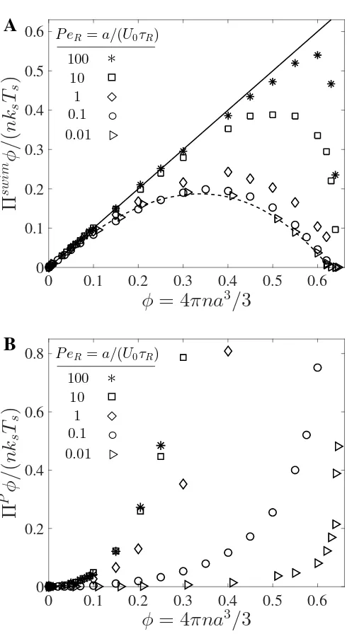
Figure 1.2: Dependence of swimmer concentration on (A) swim pressure and (B) interparticle (collisional) pressure scaled with the swim activity ksTs ≡ ζU₀2τR/6.

Data are from Brownian dynamics simulations, where the reorientation Péclet num-ber PeR ≡ a/(U0τR) is the ratio of the swimmer size to its run length. In (A), for

large PeR the data collapse on the solid line representing a linear increase of the

active pressure with concentration,Πswim= nksTs. As PeR →0 the swim pressure

decreases with increasing concentration and agrees withΠswim = nksTs(1−φ−φ2)

(dashed curve) (Takatori and Brady,Phys Rev E, 2015). In (B), the collisional pres-sure increases monotonically with concentration for all PeR.

(33)

φ

= 4

π

na

3

/

3

0 0.1 0.2 0.3 0.4 0.5 0.6

Π

a

ct

φ

/

(

n

k

s

T

s

)

0 0.2 0.4 0.6 0.8

1 P eR=a/(U0τR)

1 10 100 +

⋄

[image:33.612.174.419.85.293.2]

◦

×

∗

⊲

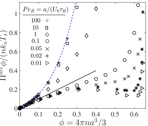
0.01 0.02 0.05 0.1

Figure 1.3: NonequilibriumΠact-φphase diagram, whereΠact =Πswim+ΠPand is scaled with the swim activity ksTs ≡ ζU₀2τR/6. Data are from Brownian dynamics

simulations, where the reorientation Péclet numberPeR ≡ a/(U0τR) is the ratio of

the swimmer size to its run length. The solid line represents a linear increase of the active pressure with concentration,Πact = nksTs. The dashed blue curve is the

Carnahan-Starling equation of state for Brownian hard-spheres. ForPeR < 1/3 we

observe a negative ‘second virial coefficient,’ and forPeR . 0.03 a non-monotonic

pressure variation (analogous to a ‘van der Waals loop’).

Active pressure

The total pressure of active matter (in the absence of hydrodynamic interactions) is given by P = pf +Πact, whereΠact = Πswim+ΠP is the ‘active pressure’ and

pf is the solvent pressure (which is arbitrary for an incompressible fluid and is set

to zero). Comparing Figs 1.2A and 1.2B, we have a competing contribution to the active pressure. Namely, as we increase swimmer concentration,Πswim decreases (destabilizing) whereasΠP increases (stabilizing). This competition may result in what would be a negative ‘second virial coefficient’ B2, which implies two-body attractions and the possibility of a ‘gas-liquid phase transition.’ Attractions may give rise to a non-monotonic variation of pressure with concentration, known as a “van der Waals loop.”

(34)

and dilute phases.

As shown in Fig 1.3, at low φ all data collapse onto the ideal-gas swim pressure given by Eq 1.2. At high PeR, the interparticle pressure dominates and the total

pressure increases monotonically withφ. Because the swimmers take small swim steps and reorient rapidly for PeR 1, the active pressure agrees well with the

Carnahan-Starling equation of state for passive Brownian hard-spheres (see blue dashed curve in Fig 1.3). As PeR is reduced below ∼ 0.03, we observe a

non-monotonic pressure profile resembling a van der Waals loop. The decrease inΠact for PeR 1 is caused by the reduction in swim pressure due to the particles’

tendency to form clusters, reducing the average distance they travel between re-orientations. As φ approaches close packing, the swim pressure decrease to zero (see Fig 1.2A) but the active pressure necessarily increases because the interpar-ticle (excluded volume) pressure diverges to infinity (Fig 1.2B). It is in this limit where experiments and computer simulations [19, 62, 64, 65, 66, 79] have ob-served the self-assembly of active systems into dense and dilute phases resembling an equilibrium liquid-gas coexistence.

When designing an experiment or computer simulation, the size of the container or simulation cell must be large compared to the run length of the swimmers, U0τR.

A smaller container artificially reduces the swim pressure because the container size enters as a new length scale in the problem and diminishes the distance the swimmers travel between reorientations [52, 58, 80].

We now understand the behavior of the active pressure for small and large values of PeR; in the next subsection we discuss a simple model to predict the phase

separa-tion for all values of density andPeR.

PVT phase diagram

Given an analytical expression forΠswim andΠP [74], the active pressure for small PeRis

Πact =nksTs

1−φ−φ2+3φPe_R(1− φ/φ0)−1. (1.4)

(35)

φ

= 4

π

a

3

n/

3

0.2 0.3 0.4 0.5 0.6

P

e

R

=

a

/

(

U

0

τ

R

)

10-3

10-2

10-1

Π

a

ct

φ

/

(

n

k

s

T

s

)

0.02 0.07 0.22 0.71 2.32 7.62 25.01 82.09

Wysocki, Winkler, Gompper (2014)

[image:35.612.162.445.81.310.2]

•

◦

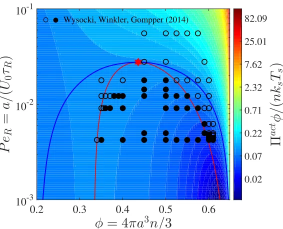
Figure 1.4: Phase diagram in the PeR − φ plane for a 3D active system.

Color-bar represents the magnitude of the active pressure scaled with the swim activity ksTs ≡ ζU₀2τR/6, and the blue and red curves are the binodal and spinodal,

respec-tively. The critical point is shown with a red star. The open and filled symbols are simulation data (Wysocki, Winkler, and Gompper,Europhys Lett, 2014) with a homogeneous and phased-separated state, respectively.

spherical swimmers not in confinement, so there is no such wall interaction and we can use Eq 1.4 to predict the phase behavior.

Figure 1.4 shows the phase diagram in thePeR −φplane, where Eq 1.4 was used

to determine the regions of stability from the spinodal condition, ∂Πact/∂φ = 0. This is given by the red curve in Fig 1.4 that passes through the extrema of each constant-pressure isocontour (“isobar”). At the critical point (red star in Fig 1.4), ∂Πact/∂φ= ∂2Πact/∂φ2 = 0. In 3D the critical volume fraction φc ≈ 0.44, active pressure Πact,cφc/(nksTs) ≈ 0.21, and reorientation Péclet number Pec_R ≈ 0.028,

values consistent with our BD simulations and simulation data of others [82, 72, 73]. No notion of free energy is needed to obtain the spinodal and critical point— they are purely mechanical quantities.

(36)

mechanical balances [5, 74]: n(∂ µact/∂n) = (1− φ)(∂Πact/∂n). This definition, which makes no approximation other than solvent incompressibility, agrees with the true thermodynamic chemical potential for molecular or colloidal solutes in so-lution [54]. Active systems with a small reorientation timeτR →0 not only behave

similarly but are equivalent in dynamics to that of passive Brownian particles. If we placed active swimmers behaving identically to passive Brownian particles behind an osmotic barrier, we would not be able to distinguish one from the other. Because the form of the chemical potential and pressure are equivalent for the two systems, we interpret µact as a natural definition and extension of the chemical potential for nonequilibrium systems, and use it to compute and define a “binodal.”

Simulations of Wysocki et al [82] agree well with the spinodal of this model as shown by the location of the transition from the homogeneous (open symbols) to phase-separated (filled symbols) states. In 2D, simulation of Speck et al [73] sug-gest that the transition occurs near the binodal [74]. Figure 1.4, which contains no adjustable parameters, predicts that active systems prepared outside the binodal (blue curve) are stable in the homogeneous configuration and do not phase sepa-rate. Between the spinodal and binodal, the system is in a metastable state and does not spontaneously undergo a spinodal decomposition. In a simulation the system may stay in the homogeneous phase unless an artificial nucleation seed causes the system to transition to the globally-stable phase [64].

From Fig 1.4, we see that the reorientation Péclet number plays an important role in the phase behavior of active systems. In addition to a ratio of the particle size to its run length, we can use the swim activityksTs ≡ ζU₀2τR/6 to rewrite the reorientation

Péclet number as PeR ≡ a/(U0τR) = ζU0a/(6ksTs), which is interpreted as a ratio

of the interactive energy of the swimmer – force times distance, ζU0 × a– to the swim activityksTs.

Figure 1.4 reveals that phase separation becomes possible for small PeR =

ζU0a/(6ksTs), or high Ts. This is opposite to a classical thermodynamic

sys-tem where phase transitions occur at low sys-temperatures. Yet some syssys-tems like temperature-responsive polymers display a lower critical solution temperature (LCST) transition, where phase separation becomes possible at high temperatures [83]. A possible interpretation for active matter systems exhibiting an LCST is that the particle effectively becomes larger in size and thus has less space available for entropic mixing as PeRdecreases (i.e., run length increases).

(37)

matter in the context of phase separation and provide a justification that Ts can

indeed be interpreted as a temperature under certain situations.

1.8 Temperature of active matter?3

Because the swim pressure has been a useful concept to predict the collective be-havior of active matter, a natural question and extension pertains to the temperature of active matter. Wu and Libchaber [84] observed anomalous behavior of passive Brownian particles when placed in a suspension of run-and-tumbleE. coli, and at-tributed the particles’ enhanced translational diffusivity to the collective motion of the bacteria. Subsequent studies like Loi et al [85] introduced an interesting notion of using passive tracer particles as a ‘thermometer’ to measure the ‘effective tem-perature’ of an active suspension, as many experimental, numerical, and theoretical studies reported on the enhanced hydrodynamic tracer diffusion in a bacterial sys-tem [86, 87, 88, 89, 90, 91, 92, 93]. However, the use of an effective temperature of nonequilibrium active matter is not valid in general [49], and it is unclear whether a mapping between the effective temperature and the thermodynamic temperature exists at all.

To understand the ‘temperature’ of active matter, we shall consider a simple ex-periment involving the mixing of two systems of active swimmers with a different activity, ksTs ≡ ζU₀2τR/6 [94]. Suppose a system of “hot” active swimmers with

(ksTs)H is initially separated from “cold” swimmers with (ksTs)C. When the

sys-tems are allowed to mix, the swimmers with different activities collide and displace each other, but they never share their intrinsic kinetic activity (ksTs) upon

colli-sions. Even after a very long time, the system is still composed of “hot” and “cold” swimmers with no equilibration of the ‘temperature,’ or the activity. This is oppo-site to a purely passive Brownian suspension or a molecular fluid, which thermally equilibrates when systems of different temperatures mix.

For a passive tracer particle in a sea of active swimmers, the motion of the tracer depends on the swimmers’ reorientation Péclet number PeR ≡ a/(U0τR). For

PeR 1 the swimmers take small swim steps and they repeatedly displace the

tracer particle of order the step size ∼ O(U0τR) upon collisions. In this limit the

tracer particle can sense the activity or ‘temperature’ of the swimmers via collisions because the fluctuations it receives come from the swimmers’ activity (plus a con-tribution from the solvent’s thermal fluctuations), allowing it to behave as a

(38)

mometer’ for the activityksTs = ζU₀2τR/6. In this sense a suspension of swimmers

with small run lengthsU0τR < a can be mapped to a purely Brownian suspension

with an effective ‘temperature’ksTs4.

In the other limit ofPeR 1, the swimmer collides with the tracer and continues

to translate until the tracer moves completely clear of the swimmer’s trajectory. The tracer receives a displacement of ∼ O(a) upon colliding with a swimmer, not the run lengthU0τR. Unlike the limit ofPeR 1, the tracer cannot act as a

thermome-ter because it only receives a displacement of its sizea, even though the swimmers actually diffuse with their swim diffusivityDswim ∼U₀2τR. In this limit, the

reorien-tation Péclet numberPeR ≡ a/(U0τR) is the quantity that gets shared between the

swimmers via collisions [74], and the activity ksTs ≡ ζU₀2τR/6 cannot be mapped

to the thermodynamic temperature.

Here we have focused on a simple system of active Brownian particles with a ho-mogeneous intrinsic swim speed and reorientation time (i.e., activity), which lends itself to a thermodynamic perspective. There is also a continuum perspective which allows slow variations in space and time, and this engenders the notion of interpret-ing the swim force as a body force, as described next.

1.9 Swim force as an ‘internal’ body force

Recent discussions [81, 95] have questioned the validity of the active pressure as a true thermodynamic pressure and a state function. Solon et al [81] derived an expression for the pressure on the bounding walls of a container when a local, ex-ternal torque was applied to each active particle colliding into the wall. They report that the wall pressure depends on the detailed form and nature of the local torque and conclude that the pressure of active matter thus cannot be a state function in general because the force per area on the bounding walls is not necessarily equal to the swim pressure far away from the wall, especially when polar order is present in the system.

A recent work resolved this concern by using both a global force balance and a continuum-level derivation [96]. We established in Sec 1.2 that it is permissible and essential to interpret the self-propulsion of an active particle as arising from a swim force,Fswim = ζU0qfor an active Brownian particle, whereqis the unit orientation vector specifying the particle’s direction of swimming. For an active particle in the

4_{For active Brownian particles, this contribution is in addition to the thermal} _k

BT that gets

(39)

absence of any external forces or torques, the average swim force is zero because the particle’s orientation distribution is uniform: hFswimi = ζU₀hqi = 0. If we have an external orienting torque on the particles that result in polar order, then the swimming orientations are not uniform, hqi _, 0, and thus there is a nonzero average swim forcehFswimi_, 0. This nonzero average swim force may arise from an intrinsic mechanism internal to the body, so it is to be construed as an ‘internal’ force. Yet, this internal average swim force behaves equivalently to an external body force such as gravity [96]. Thus the true mechanical pressure exerted on a boundary is a sum of the swim pressureplusthe ‘weight’ of the particles (or the average swim force), and the active pressure is indeed well-defined and independent of interactions with boundaries.

A microscopic theory [80] based upon moment expansions of the Smoluchowski equation revealed that the particle concentration and hence the force exerted on the wall depends on boundary curvature, flux conditions at the surface, etc., which agree with Solon et al [81]. Inclusion of the ‘internal’ body force (i.e., nonzero average swim force) into the momentum balance shows that the force per unit area on the boundary plus the integral of the internal body force is equal to the active pressure far from the boundary.

The swim pressure perspective allows researchers to analyze the effects of external forces like gravity or orienting torques in a homogeneous suspension, and then use these results to subsequently predict the inhomogeneous behavior of the active system. External gravitational fields or torques do not cause the active particles to generate their own mechanical pressure, but an external field does affect the swim pressure [57].

We motivated this development assuming that the particles have polar order and hence a nonzero hFswimi. However, we may also have a density-dependent or spatially-varying intrinsic swim velocityU0(x) and reorientation timeτR(x), due to

a variation in fuel concentration, for example. This results in a nonzerohFswimi = −(1/n)σswim · ∇log(U0τ_R) [94], which must then appear in the global force bal-ance and in the continuum description to compute the pressure of active matter. Therefore, the key is to have a nonzerohFswimi, not necessarily any polar order.

(40)

and modify the swim pressure. However, the swim pressure would still be a funda-mental concept to explain the phase-separating behavior of active systems.

Lastly, a microscopic perspective [80] allows any scale variation and shows the importance of another micro-length scaleδ ∼√D0τRthat allows the swim pressure

to emerge naturally. This perspective allows the swimmers’ run length to be on the order of the body size (or smaller) and gives rise to interesting phenomena like the Casimir effect [97].

1.10 Conclusions

In this introd