Statistical analysis of body surface electrocardiographic maps in ischemic heart disease

Statistical analysis of body surface electrocardiuraphic maps

in ischemic heart disease

by

Anthony James Bell MB BS FRACP

Faculty of Medicine and Pharmacy Department of Medicine

submitted in fulfillment of the requirements of the degree of

Doctor of Medicine University of Tasmania

August 1993

This thesis contains no material that has been accepted for the award of any other higher degree or graduate diploma in any tertiary institution, and this thesis contains no material constructed by another person except where acknowledged.

Preface

After becoming interested in body surface mapping in the coronary care unit I came to realize that diagnosis of acute myocardial damage by body surface map was simple and appeared more accurate than with standard 12 lead electrocardiography. This applied especially late at night in the coronary care unit, when recorded maps lead to rapid accurate diagnosis. In fact, in a small number of patients with completely normal standard electrocardiograms, the body surface map showed a myocardial infarction. The method of body surface mapping was quick, efficient and clearly better than the standard methods in some cases. The body surface mapping method developed by Drs David Kilpatrick and Stephen Walker in the University of Tasmania clearly had clinical potential. Drs Kilpatrick and Walker taught me computer methods and provided the background knowledge to proceed with this thesis. This thesis attempts to demonstrate the clinical usefulness of body surface mapping.

The thesis is composed of 13 chapters. Chapters 1 to 5 are introductory in nature and outline the history and concept of body surface mapping. the changes in the standard electrocardiogram related to myocardial infarction, and summarize the statistical methods used in this thesis. After each chapter is an appendix which contains tables then the figures relevant to that chapter.

The clinical study chapters - 6 through 12 - have the same format. There is an introduction reviewing the clinical problem followed by a brief methods section. The results are presented then discussed with reference to the literature on the subject. Each chapter is followed by an appendix section containing the tables and then the figures for that chapter.

infarction. Chapter 6 is a combined effort of Dr S. J. Walker, Dr M. G. Loughhead, Dr D. Kilpatrick and myself. The initial idea of the interpretation of the ST segment body surface maps was conceived by Dr M. G. Loughhead and Dr D. Kilpatrick. The study subgroups patients with acute inferior wall myocardial infarction and relates the body surface map appearance to the prognosis in a learning and test set of patients. The data has been published as two papers. (Walker SJ, Bell AJ, Loughhead MG, Lavercornbe PS, Kilpatrick D: Spatial distribution and prognostic significance of ST segment potentials in acute inferior infarction determined by body surface mapping. Circulation 1987;76:289-297 and Bell AJ, Loughhead MG, Walker SJ, Kilpatrick D: Prognostic significance of ST potentials determined by body surface mapping in inferior wall acute myocardial infarction. Am J Cardiol 1989;64:319-323)

Chapter 7 studies the natural history of the body surface map in inferior wall myocardial infarction and relates the natural history to the prognosis. This study has been published. (Bell AJ, Walker SJ, Kilpatrick D: Natural history of ST-segment potential distribution determined by body surface mapping in patients with acute inferior infarction. J Electrocardiol 1989;22:333-341)

Chapter 8 relates the ST segment body surface map to the loss of QRS complex voltage in acute inferior wall myocardial infarction. This study is derived from work by Dr D. Kilpatrick and myself in which Dr Kilpatrick is the major author. The chapter is included for completeness. The work has been published. (Kilpatrick D, Bell AJ: The relationship of ST elevation to eventual QRS loss in acute inferior myocardial infarction. J Electrocardiol 1989;22:343-348)

Chapter 9 studies the body surface map in acute anterior wall myocardial infarction and relates the map to prognosis.

voltage in acute anterior wall myocardial infarction. (Bell AJ, Nichols P. Briggs C, Kilpatrick D: Prognostic significance of ST potentials determined by body surface mapping in anterior wall acute myocardial infarction. J Electrocardiol (1993 in press))

Chapter 11 studies the body surface map in patients with a normal electrocardiogram with or without coronary artery disease. The patients all underwent coronary angiography to determine the presence or absence of coronary artery disease. The studies determined if detailed analysis of the body surface map would detect coronary artery disease in patients with no history of myocardial damage. The mathematics and computer program for the Eigenvector method was developed in the University of Tasmania by Ms Lydia Piggot specifically for this purpose

Chapter 12 is a study of the accuracy of the body surface map and the inverse transformation in .predicting the loss of myocardial cells as measured by thallium scanning. (Bell AJ, Ryan A, Ware R, Walker SJ, Kilpatrick D: Derived epicardial ST segment potential distribution compared to the resting distribution of thallium scintigraphic defect in acute myocardial infarction. Am J Noninvas Cardiol 1991; 5: 273-279). This chapter leads into a new area of body surface mapping, the clinical application of the inverse transformation.

Chapter 13 summarizes the thesis and plans new directions and applications for body surface mapping.

The list of references used is documented after chapter 13.

The appendix after the bibliography contains the more recent papers published on body surface mapping by myself and Dr. Kilpatrick.

the Coronary Care Unit in the Department of Critical Care Medicine. Special thanks are due to the dedicated "mappers" Dr A. Duffield, Dr \V. Herbert, Sr J. Walsh and Sr C. Briggs.

A bst ract

Body surface electrocardiographic mapping is a technique for recording the thoracic electrical potentials generated by the cardiac cycle and transmitted to the body surface. The body surface map emphasizes the spatial distribution of the cardiac electrical potentials rather than the time magnitude relationship of the standard electrocardiogram. The body surface map contains more information than the standard electrocardiogram and in a different format. This thesis addresses the following questions:

1. is the additional information contained in the body surface map of clinical significance in myocardial infarction ?

2. is the display format and thus the application of topographical statistics of clinical benefit in myocardial infarction?

3. is the addition information able to detect coronary artery disease in patients presenting with chest pain ?

Detailed analysis of the body surface map in acute inferior wall myocardial infarction predicted the clinical course of the patient, one map pattern being associated with a high mortality and morbidity, giving a guideline to immediate therapy. The area of ST segment elevation corresponds to the the area of eventual Q wave formation in acute inferior wall myocardial infarction. Thus the body surface map may be useful in assessing reperfusion by thrombolytic agents in acute myocardial infarction.

The body surface. mapping was unable to differentiate patients with and without coronary artery disease who had normal standard electrocardiograms. The body surface map was useful in differentiating patients with acute or old myocardial infarction from normal patients but did not detect coronary artery disease in the absence of myocardial damage.

The information content of the body surface is increased if an accurate inverse transformation can be used to calculate the epicardial potentials in the clinical situation. To prove that epicardial potentials are. accurately calculated, comparison of the area of myocardial damage to the calculated epicardial area of ST segment elevation was made using thallium scanning. This demonstrated a good correlation demonstrating that the inverse transformation was accurate. The technique is adding a new dimension to the understanding of the origin of the electrocardiogram.

Table of Contents

Title page

Preface ii

Abstract vi

Chapter 1: History of body surface electrocardiographic mapping 1

The concept of the body surface electrocardiographic map 3 Advantages of body surface electrocardiographic map 4

The aim of this study 4

Chapter 2: Electrocardiographic changes in myocardial infarction 6 Chapter 3: Data collection in body surface mapping 21

Introduction to body surface mapping methods 22 Description of body surface mapping method 26

Data display 28

Chapter 4: Data analysis in body surface mapping 37

Methods of data analysis 38

Methods of grouping electrocardiographic body surface maps 45 Multivariate analysis of body surface maps 49

Chapter 5: Data collection 59

Data collection for myocardial infarction studies 60 Data collection of angiogram controlled studies 62

Chapter 6: ST segment potential distribution in acute inferior wall

myocardial infarction 64

Introduction 65

Methods 66

Results 68

Discussion 73

Table of Contents

Chapter 7: History of ST segment potential distribution in inferior wall

myocardial infarction 87

Introduction 88

Methods 89

Results 92

Discussion 94

Conclusion 97

Tables and figures 98

Chapter 8 ST segment elevation to eventual QRS loss in inferior wall

myocardial infarction 108

Introduction 109

Methods 109

Results 110

Discussion 111

Tables and figures 115

Chapter 9: The prognostic significance of the ST segment in anterior

infarction 117

Introduction 118

Methods 119

Results 121

Discussion 124

Conclusion 127

Tables and figures 129

Chapter 10: ST segment elevation to eventual QRS loss in anterior wall

myocardial infarction 135

Table of Contents

Results 139

Discussion 142

Tables and figures 146

Chapter 11: Detection of coronary artery disease by statistical analysis of

body surface maps. 152

Introduction 153

Methods 153

Results 156

Discussion 158

Tables and figures 160

Chapter 12: Derived epicardial ST segment potential distribution 172

Introduction 173

Methods 173

Results 177

Discussion 179

Tables and figures 183

Chapter 13: Future of body surface electrocardiographic mapping 188 Body surface and standard electrocardiography 189 Problems with body surface electrocardiographic map 190 The future of body surface electrocardiographic map 191

Chapter 1

History of and introduction to

A brief history of body surface electrocardiographic mapping

The electrocardiogram has been a major tool in the diagnosis of coronary artery disease for over 75 years. Since the initial recording of the human electrocardiogram by Waller in 1887 [Waller 1887], the development of the string galvanometer in

1913 [Einthoven 1913] and the advancement of the PQRST terminology to describe the electrocardiogram by Einthoven [Cooper 1986] enabled the electrocardiogram to become a standard tool in clinical cardiology.

As early as 1888 Waller had sketched the electrical potential over the entire thoracic surface of man. The recording and displaying of the entire thoracic electrocardiographic potential became known as body surface mapping. The first simultaneous recording over the thoracic surface was by Nahum et al. in 1951 [Nahum 1951]. In 1965, Taccardi and his team at the University of Parma, Italy, published hand drawn isopotential maps of the surface distribution during the QRS complex [Taccardi 1963]. These workers had manually recorded 80-600 electrocardiographic leads in patients then constructed hand drawn isopotential maps. Horan et al. developed a belt system [Horan 1963], derived from the work of Nelson [Nelson 1957], to record the potentials of the torso of a dog, and used a small computer to plot isopotential body surface maps.

In recent years with the introduction of multi-channel recorders, computerized data analysis and graphics, the methods of body surface electrocardiographic map recording have become simpler. Many groups have now studied body surface electrocardiographic maps in relationship to normal cardiac physiology and cardiac pathophysiology. Normal atrial activation and recovery [Mirvis 1980, Taccardi

Spach 1979a, Spach 1979b, Abildskov 19761 have been well described. The body surface map in myocardial infarction has been described by many workers [Flowers 1976a, Vincent 1977, Flowers 1976b, Toyama 1980, Pham-Huy 1981], but the early map changes in acute myocardial infarction have been less well studied [Muller 1978, Maroko 1972, Muller 1975, Selwyn 1977, Mirvis 1977] . The early studies of the body surface map changes in acute myocardial infarction used maps recorded hours after the onset of acute myocardial infarction. For example, the study of Montague et al. recorded maps from patients a mean of 76 hours after the onset of acute myocardial infarction [Montague 1983]. The early changes of acute myocardial infarction, although well described for the 12 lead (standard) electrocardiogram, have never been examined in detail in large numbers of patients.

The concept of the bodv surface electrocardiographic map

understanding the body surface map. The body surface map is a spatial electrocardiogram with the emphasis on the distribution of potentials. The standard electrocardiogram is a time magnitude recording of the cardiac electrical field at particular body surface sites.

Advantages of body surface electrocardiographic map

Mirvis has recently reviewed the presumed advantages of body surface mapping over standard electrocardiography [Mirvis 1987]. These include the following features:

1: analysis of spatial as well as temporal features of the cardiac electrical cycle; 2: detection of information not projected to localized torso regions; and

3: the close correlation of body surface map information and epimyocardial events [Myerburg 1989].

In spite of the theoretical and practical advantages of body surface mapping in chronic myocardial infarction and exercise testing, body surface mapping has not become the clinical gold standard in electrocardiography. Indeed the acceptance of body surface mapping has been limited [Mirvis 1987].

The aim of this study

surface map using the inverse transformation [Spach 1979al.

Chapter 2

Electrocardiographic changes

in acute myocardial infarction

roduct ion to the elect roca rdio:ram

The electrocardiogram is a measurement on the body surface of the electrical activation and the electrical recovery of the heart. The electrical potentials measured by the electrocardiogram are generated by the heart and are due to cellular membrane ion fluxes. The ion flux generates a current which in turn generates extracellular fields within and on the surface of the body. The cardiac current flow causes the electrocardiographic potentials on the skin surface, measured by the electrocardiogram. Each electrocardiographic measurement is the potential difference between two points on the skin surface measured over a complete cardiac cycle of depolarization and repolarization. In humans the heart is usually in a constant position in the thorax, has a constant structure and generates a consistent cunent flow, and therefore the electrocardiogram is of a uniform nature. By using consistent body surface sites to measure the cardiac generation of electrical potentials, an electrocardiogram of constant pattern is obtained. Alterations in the heart tissue lead to changes in the electrical current generated by the heart. The electrical potential changes are measured by the electrocardiogram and correlate to changes in the heart structure and function. Over the last 100 years studies correlating the changes in the electrocardiogram with types of heart disease have developed the electrocardiogram into a powerful diagnostic tool. For example, the initial and characteristic changes in the electrocardiogram during acute myocardial infarction are used to diagnose and plan treatment for the patient.

Terminology describing the electrocardiogram

The electrocardiogram consists of 12 measurements of electrical potential differences. Each measurement is between two points on the skin surface. Each site of measurement is called an electrocardiographic lead. The various features of an electrocardiographic lead are named as shown in figure 1. The initial wave, the P wave, is the electrical potential measure at the time of atrial depolarization. The QRS deflection is the electrical depolarization of the ventricular muscle: the Q wave

is an initial negative deflection in the QRS deflection; the R wave is the initial positive deflection in the QRS complex; and the S wave is a negative deflection after a positive deflection. An R' is a second positive deflection. An S' is a further negative deflection following a previous S wave. The T wave is the repolarization of the ventricular muscle. The segment of the electrocardiogram between the P wave and the QRS deflection is the PR interval. The segment between the QRS deflection and the T wave is the ST segment. The segment between the T wave and the P wave of the next beat is the TP segment. The J point is the point at which the QRS deflection becomes the ST segment.

The baseline or zero potential of the electrocardiogram

current electrical component. The use of alternating current amplifiers means that

the signal is recorded about zero and that actual potential differences existing during

the TP, PQ, and ST intervals cannot be derived. The difference between the steady

levels, for example the ST-TP difference, can be measured but whether the

difference is due to primary ST elevation or TP depression would require direct

current amplifiers to elicit. This has relevance for this thesis in which ST changes

are of major importance.

The generation of the cardiac electrical field

Electrocardiographic potentials arise from ion fluxes that occur during

depolarization and repolarization of myocardial cells. The alteration of the electric

potentials is known as the action potential. The action potential of a single

myocardial cell is shown in figure 2. These intracellular ionic currents generate

extracellular potential fields on and around the heart and thus on the surface of the

body. A complete discussion of the generation of the electrocardiogram is beyond

the scope of this thesis.

The measured potentials of the body surface electrocardiogram are influenced by

many factors. The initial factor is the generation of the cardiac current flow known

in total as the cardiac generator as shown in figure 3 [Mirvis 1988].

The action potential of the heart cells is caused by movement of ions across the

cell boundaries resulting in potential differences between the inside and outside of

the cell. During cardiac excitation intracellular potentials exist between electrically

connected cells. Each cell is surrounded by a relatively impermeable high resistance

membrane. This cell structure favours conduction through one end of the cell to the

end of the next cell. Thus current flow is along the direction of the fibre. With cell

negative potential than the neighbouring cells in the rest phase. Current flows in the intracellular space through the cell connections from regions of higher to regions of lower potential. The intracellular current flow determines the extracellular potentials [Spach 1979a]. The extracellular potentials are transmitted to the body surface as a potential of about 1% of the amplitude of the transmembrane voltages. The transmitted potentials have a relationship to the cardiac events although the relationship is influenced by factors that alter the transmission to the body surface (figure 3) [Mirvis 1988a].

The QRS complex in the electrocardiogram

The QRS complex arises from the excitation of the ventricular muscle. In the normal heart the cardiac electrical conducting system causes the cardiac muscle to be excited almost simultaneously at a number of right and left ventricular sites. Each muscle fibre undergoes an electrical discharge known as the action potential. The QRS complex of the electrocardiogram represents the depolarization of all the ventricular muscle with each electrocardiographic lead recording at that body surface site the sum of the electrical potential differences generated by cellular depolarization. The general pattern of the QRS complex is dependent on the heart geometry, depolarization sequence, body tissue conduction and the shape of the body surface (figure 3).

The ST segment in the electrocardiogram

shown in the action potential of a single muscle fibre (figure 2). The absence of ST segment deviation from the baseline implies the absence of significant current flow during slow ventricular repolarization. This condition is not always fulfilled. If there is a slight difference between cells in the timing of the end of the QRS complex then there is J. point deviation and early deviation of the ST segment. As a result the ST segment deviation is usually measured 80 milliseconds from the J point. The duration of the ST segment tends to parallel the duration of the action potential. Rate dependent changes in the duration of the ST segment reflect rate dependent changes in the duration of the ventricular action potential [Lepeschkin 1953]. The duration of the ST segment may vary with disorders of calcium, thyroid activity and catecholamine levels.

Normal values for the deviation of the ST segment from the TP segment (the zero potential reference) are less than 20 pV for the limb leads and higher in the precordial leads. The normal precordial lead values range from lead V1 averaging 50 ± 30 l_tV, lead V2 averaging 100 ± 60 t_tV to lead V6 averaging 10 ± 10 p.V.

The T wave in the electrocardiogram

The electrocardiogram in acute mvocardial infarction QRS changes

In myocardial infarction there is a loss of myocardial tissue. The loss of tissue, with replacement of the electrically active tissue by electrically inert tissue, alters the QRS complex. The loss of tissue results in the loss of the electrical forces in the region of the infarction. A recording electrode may record an alteration in electric potentials. The summation of all the electrical forces remaining may be negative, causing the initial deflection of the recording to be negative and creating the initial Q wave characteristic of acute myocardial infarction. However if the summation of the remaining voltages remains positive a reduced voltage is recorded. Thus loss of R wave height is a marker of myocardial infarction on the standard electrocardiogram. The most obvious sign of acute myocardial infarction is the development of new Q waves, while reduction in the R wave magnitude is a less obvious sign of acute myocardial infarction [Horan 1971]. Distinguishing a normal R wave from a reduced R wave in acute myocardial infarction is difficult, especially when a pre-infarction electrocardiogram is not available.

The loss of QRS complex is related to the site and the size of the myocardial damage [Bar 1984]. There may be associated loss of conduction through damage to specialized cardiac electrical .conduction system fibres, with further distortion of the QRS complex. The classical standard 12 lead electrocardiogram finding of pathological Q waves occurs when the infarction involves tissue which is depolarized in the first 40 milliseconds of the onset of the QRS complex. Otherwise the infarction pattern is found as a notching of the R wave or loss of R wave voltage. The position of the lead showing the loss of R wave or Q wave development has a relationship to the area and size of the myocardial damage.

infarction Q wave formation occurs though the Q wave formation may not be detected by the standard 12 lead electrocardiogram; but it may be detected by body surface mapping [Montague 19861. This is thought to be due to delayed activation of the area of damaged muscle such that the area was electrically silent at the onset of the QRS complex [Miller 1978, Daniel 1971].

ST segment changes

ST segment displacement is due to either systolic or diastolic injury currents or both. The systolic injury current is due to the shortening and decreased amplitude of the action potential after injury. This causes intracellular systolic currents to flow from the normal to ischaemic areas, a true ST segment elevation. Secondly loss of resting membrane potential produces a diastolic injury current flow in the intracellular spaces from the ischaemic to the normal cells, which is true TP depression but registers on the standard electrocardiogram as ST segment elevation. TP segment depression is recorded on the electrocardiogram as ST segment elevation because the TP segment is the baseline (zero) potential against which other potentials are measured.

The type of ST segment deviation that occurs with myocardial injury varies with the site of the injury. The usual explanation for this phenomenon is that in subendocardial damage in the anterior wall of the heart the current flow is away from the recording electrode on the anterior chest wall and thus there is ST segment depression. If the injury involves the epicardial surface then the current flow during the ST segment is towards an overlying electrode and ST segment elevation is seen [Macfarlane 1989].

Associated with ischaemia there is a conduction velocity decrease and activation of the ischaemic myocardial is delayed. Repolarization of damaged tissue is altered, with the differences between the ischaemic and non-ischaemic action potentials causing secondary T wave changes. The delayed activation may cause the T wave inversion.

ST segment change indicates the area of infarction and size of infarction

Zmyslinski 19791.

Reciprocal ST segment changes

ST segment depression always occurs in the presence of ST segment elevation and can be either the result of the process which caused the injury current responsible for the ST segment elevation (true reciprocal ST segment depression), or due to the presence of an additional area of injury in another location in the heart causing primary ST segment depression. There has been debate about the prognostic value of detection of reciprocal change in the ST segment for acute inferior wall myocardial infarction [Roubin 1984, Wasserman 1983, Croft 1984, Shah 1980. Cohen 1984, Ferguson 1984, Goldberg 1981, Gibson 1982, Gelman 1982. Lembo

1986, Stafford 1986, Hlatky 1985] and for acute anterior wall myocardial infarction [Myers 1949, Pichler 1983, Haraphongse 1984, Quyyumi 1986].

Persistent ST segment elevation after myocardial infarction

In 60% of acute anterior wall myocardial infarction and 5% of acute inferior wall myocardial infarction there is persistent ST segment elevation [Shah 1980]. The ST segment elevation is related to an area of the myocardium with asynergy [Bar 19841. The persistence of the ST segment elevation relates to dyskinesis [Aryan 1984]. The aetiology of the persistent ST segment elevation is unknown.

Further clinical causes of ST segment elevation

Secondary ST segment deviations

These deviations relate to changes in the uniformity of depolarization and repolarization that can occur with conduction delays. Such changes are usually associated with T wave variation due to the lack of uniformity in the repolarization of the heart muscle [Macfarlane 1988].

Normal variant ST segment elevation

This implies that the ST segment shift is due to the shortening of the ventricular action potentials in some epicardial regions. The condition is found in normal people, more so in blacks, and is not associated with a worse prognosis in the individual [Kambara 1976, Spodick 1976]. Isoproterenol and exercise may abolish the ST segment elevation by abolishing the differences between action potentials [Spodick 1976, Morace 1979].

Pericarditis

Summary

Figure 1 : Terminology used to describe the normal electrocardiogram wave forms

R wave

The standard terminology applied to the electrocardiogram over a single cardiac cycle. The P wave is atrial depolarisation, the QRS complex

100 200 300 40 500 potential

difference

-45

-60

resting membrane potential 30

15

0

-15

-30

rapid ventricular repolarization ventricular

depolarizatio

slow ventricular repolarization

time (milliseconds) Figure 2 : Action potential of a single cardiac muscle filKe

The x axis is time in milliseconds. The y axis is the potential difference between the inside of the myocardial cell and the outside of the

Figure 3: Generation of the body surface electrocardiographic man

sequence of events

electrocardiographic pattern cardiac generator affected by

cardiac activation sequence cardiac structure

electric field

transmission factors thoracic structure body surface potentials

lead placement

body surface map

Chapter 3

Data collection in

Introduction to body surface mapping methods

Data collection in body surface mapping is more difficult than in standard twelve

lead electrocardiography. Where the standard electrocardiogram has 9 electrodes

applied at 9 body sites collecting 12 potential differences, our body surface map has

50 electrode sites measuring 50 potential differences. The increased electrode

application and the increased data collected creates problems with the recording and

analysis of the data. This chapter discusses the problems of electrode positioning

and data collection in body surface mapping.

The electrode position

The major factor in body surface mapping is the electrode coverage of the

thorax. The electrode array must record all relevant electrical potentials on the body

surface. To conduct studies on seriously ill patients, the electrode application

must be simple and able- to be performed with a minimum of discomfort to the

patient. Data must be recorded rapidly to avoid interference with patient care.

Different approaches that avoid interference with patient care are possible. One

solution is to use a comprehensive lead system where 125 to 250 electrodes are

applied. This electrode system covers the torso with electrodes at a high density.

The data recorded has a large redundancy of information, and failure of data

collection from one or many of the electrodes is not critical. Though the data

collected from multiple electrodes may have greater detail [Arisi 1983] the question

of a clinical advantage has not been studied. For example there is little qualitative

difference between the body surface map appearance recorded from 121 and from 85

recording electrodes [Yamada 1978]. The .disadvantages of systems with large

numbers of electrodes are the time required for application and the discomfort to the

high degree of redundancy makes analysis of the information difficult.

A second approach is to use lead subsets. This involves the application of fewer electrodes with electrode placement in selected sites. This method is based on the assumption that comprehensive lead systems have a large amount of redundant data. and that all non-redundant data can be captured by selected lead placement. Several methods have been described [Horan 1980, Barr 1983, Spach 19711. By principal component analysis Barr and coworkers developed an electrode system with 24 electrodes of a 150 electrode lead system [Barr 1983, Spach 1971]. The analysis allows calculation of the 150 leads from the 24 measured leads by linear combinations of the measure voltages at each of the 24 leads. Green and coworkers used a data reduction algorithm to reduce a measured 192 electrode array to a 32 electrode array body surface map [Green 1987]. When a 32 electrode array was used to record and body surface map and compared to the 192 lead an-ay body surface map, the root-mean-square error between the two maps was low, and the correlation between the two maps was extremely high. The conclusion is that the available data can be recorded using a 32 lead array of electrodes provided the electrodes are placed appropriately. Interestingly, in a companion study Lux, Green and coworkers used different sets of 30 electrodes including a set with no back electrodes [Lux 1979]. All sets of 30 electrodes produced estimates little different from the 192 lead body surface electrocardiographic map. Thus 30 electrodes appear to be adequate for the measurement of most of the information contained in the cardiac electrical potentials on the surface of the body.

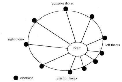
required to record the fine detail of the map ]Lux 1979, Lux 1978]. Fifty electrodes allows collection of potentials from sites not recorded by the standard 12 lead electrocardiogram. Using 50 electrodes reduces the technical burden of clinical mapping and allows ease of computation. In our mapping system the 50 electrodes are spaced around the torso with a greater density over the left precordium as shown in figure 2. This array is better than a tightly packed left precordial electrode system [Lux 1979] and standard electrocardiographic lead positions [Lux 1979]. The packing system used corrects for the eccentric position of the heart in the chest cayity. Thus the angle subtended by each electrode around the heart is approximately equal (figure 2).

The electrical reference point

The potential sensed by the electrode is the difference between the reference electrode and the recording electrode. Our system uses a calculated reference electrode. The calculation is designed to calculate the electrocardiographic reference electrode known as Wilson's central terminal [Wilson 1932]. In fact the choice of reference electrode is not important as the shape and location of the contour lines do not change [Spach 1979,. Taccardi 1962]. The choice of Wilson's central terminal, the reference point for standard electrocardiography, allows comparison with standard 12 lead precordial electrocardiography. Using Wilson's central terminal allows standard interpretation of the body surface maps.

The isoelectric (zero) baseline

baseline [Taccardi 1962]. This is the usual practice ill standard electrocardiography.

The QRS complex onset (zero time)

The continuous nature of the cardiac electrical cycle means that a zero time point is required. The onset of the QRS complex is taken as the zero time reference point. The QRS onset is automatically picked by a computer algorithm and checked manually. The data is differentiated and the location of the first value to exceed a

specific threshold derivative is found. From this point the position where the

derivative next becomes negative is found. If this position is less than 6 milliseconds

on from where the threshold value was exceeded, it is assumed that a noise spike has

been found and the search continues. Otherwise it is assumed that the point reached

is near the QRS complex peak. If no peak is found then the search is continued with a lower threshold value. Once a point near the peak of the QRS complex is found a search is continued backwards until the undifferentiated data reaches the baseline noise level. This point is the designated QRS onset. The onset of the QRS complex is difficult to pick to the nearest millisecond. The reason for this inaccuracy is the noise in the system and the gradual onset of the electrical potential. In theory the onset starts with a single myocardial fibre depolarizing and then spreading to other myofibrils. The electrical onset is a hyperbolic curve and the moment of onset is difficult to pick from the background noise [Macfarlane 1989]. In practice this means that onset picking between maps may vary by up to ±10 milliseconds, in our experience. Figure 3 represents an expanded electrocardiogram lead trace. The

over a given time period. This concept is illustrated in figure 4. Using integral maps over a short time periods, for example 20 milliseconds, makes some correction for the variation in the QRS onset. Some loss of information in integral maps is unavoidable and the clinical significance of such loss is unclear. The use of integral maps is more rational than the use of instantaneous maps. Integral maps reduce noise, especially 50 Hertz noise from mains electricity.

A second problem with the onset picking is that the QRS onset may vary by up to 40 milliseconds depending on which lead is used to pick the QRS onset [Ikeda 1985]. In our body surface mapping method the onset is picked on an average of all electrodes and the lead 12, a central thorax lead. By using a consistent reference electrode and standard method of determining the QRS onset, the variation in the QRS onset picking in minimized.

Description of body surface mapping method

by interpolation between baseline points picked manually in successive TP (baseline zero reference) segments. Baseline wander was reduced by attention to patients having normal quiet respiration at the time of recording. Complete recordings were usually made within five minutes of approaching the patient. Map displays were available within five minutes of recording the data.

To comply • with patient electrical isolation standards, the jacket, amplifiers, multiplexer and analog to digital converter are battery powered. Digital signals output from the analog to digital converter and all control systems are optically isolated. Low voltage circuitry is used in the jacket and the input buffer circuits are individually potted in epoxy resin.

Data display

The data display of a body surface map is intrinsically different from the display of a standard electrocardiogram. The standard electrocardiogram displays the electrical potential changes over time between two points on the thorax. The body surface map displays the total thoracic electrical potentials compared to a reference electrode at a single time, and successive maps show the change in time at all points on the thorax. Thus the display is different; the conventional body surface map is a representation of the thoracic surface with the potentials at the various sites displayed.

depending on the size of the patient. This data format can be use to plot map types and fed into statistical packages. The display format may be contour lines of equal potential, the isopotential map (figure 5), or a perspective map (figure 6). The isopotential or contour maps shows the overall spatial pattern and magnitudes of the potentials. Perspective maps accentuate the gradient between adjacent regions. In these studies the isopotential contour map display has been used. The display form is simple and complements the data analysis used in these studies. This format is the most commonly used in body surface electrocardiography. The data format is displayed on the unwrapped thorax. The left edge of the display is the right mid-axillary line, the centre of the display is the left mid-axillary line, and the right edge is also the right mid-axillary line. The left half of the display is the anterior thorax and the right half of the display is the posterior thorax (figure 7). With each display the maximum voltage, the minimum voltage and the site of maximum and minimum voltage are automatically calculated. The zero contour line is a bold continuous line. The positive contour lines are continuous plain lines, and the negative contour lines are dashed lines.

A time component in body surface mapping is added by producing multiple maps over the time period. In the extreme form this can be a "map movie" where. say 1 millisecond maps are displayed rapidly on the computer screen and the changing pattern of the map pattern watched in real time.

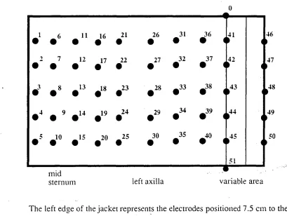
Figure 1: The configuration of the electrode jacket.

0

1

•

2

•

3

•

0

4

• 5

6

•

7

•

8

•

9

•

010

11

•

12

•

13

•

14

•

015

16

•

17

•

18

•

19

•

020

21

•

22

•

23

•

24

•

925

26

•

27

•

• 28

0

29

30

•

31

•

32

•

0

33

0

34

36

•

37

•

•

38

41

•

42

•

43

•

044

51

I

1

I

sternum left axilla variable area

The left edge of the jacket represents the electrodes positioned 7.5 cm to the right of the sternum so that the second column of electrodes is always over the mid-sternum. The neck electrode (0) is placed on the right side of the neck. The reference electrode (51) is placed on the right anteriorsuperior iliac spine. The overlap of the jacket varies with patients' size.

46

47

48

49

• electrode anterior thorax right thorax

left thorax heart

Figure 2 : Position of the electrodes around the thorax in relation to the heart position

posterior thorax

microvolts

5

4

actual onset 3

7

theoretical onset 1

time (milliseconds) 1

picked onset

3 4 5 6

true onset

Figure 3 : Expanded electrocardiogram trace and problems with onset picking

The smooth line is a theoretical representation of the electrocardiogram trace. The curving line is the usual situation. The usually recorded

Figure 4 The concept of the integral body surface map

10 15 20 25 30

C.

0 0 10 is 20 25 30

Figure 5 : Contour or isuuolculial hody surface maps

Figure 6 Perspective views of bod surface maps

Figure 7 : Contour body surface map display

anterior thorax posterior thorax

right midaxillary line left midaxillary line right midax'llary line

Chapter 4

Data analysis in

body surface electrocardiographic mappinE

Methods of data analysis Visual inspection

The simplest method of body surface map analysis is visual inspection, as per the standard electrocardiogram. The ability of visual inspection to group map patterns, and to determine the significance of patterns, was tested. In these studies all maps were inspected visually. Map differences between normal patients and patients suffering myocardial infarction are obvious. The subgroups of map patterns in patients with acute myocardial infarction were not apparent, although other researchers have claimed the opposite [Pham-Huy 1981]. Failure to recognise subgroups is due to the inability of visual inspection to group patterns uniformly and to disregard minor variations in the patterns. For example, using inferior wall myocardial infarction body surface maps, visual grouping was difficult due to the continuum of body surface maps in the condition [Walker 1987]. Although certain patterns are distinguished, a number of patterns fall in between the major patterns and could be matched to either group [Bell 19891. This problem of classification represents a problem in the biological sciences. Problems associated with intermediate patterns preventing classification are difficult to circumvent [Everitt

1974].

Difference maps

maps. The method removes subject to subject variation, and corrects for different magnitudes of potentials recorded in different subjects. Difference maps have been used in longitudinal studies of body surface electrocardiographic change over time. such as the changes occurring after acute myocardial infarction [Montague 1983. Montague 1984, Montague 19861. Unfortunately a body surface electrocardiographic map recorded before acute myocardial infarction is rare and generally unavailable in the clinical setting. In 7 years of mapping most patients admitted to the coronary care unit only two patients have pre-event maps. This factor limits the use of difference maps where the initial event occurs before a body surface map has been recorded. The time course of electrocardiographic changes occurring after an index map can be monitored by this method.

Departure maps

surface map using zeros and the outlying values. A second method of displaying a departure map is to use the number of standard deviations from the mean value of each lead and build a contour map using the number of standard deviations from normal instead of voltages. The standard deviation departure map created can have zero substituted for standard deviations less than a predetermined cut off number.

The departure map is a method of comparing the individual body surface map to a control population body surface map where the individual cannot act as the control, that is, where the event or intervention has taken place before the data are recorded. The departure map is analogous to the reference range in any clinical laboratory. In these studies the normal range was considered to be the range of plus or minus two standard deviations from the mean. This method has been used to compare body surface maps in clinical studies [Flowers 1976a, DeAmbroggi 1986a, DeAmbroggi 1986b, Ohta 1981, Suzuki 19841.

Statistical comparisons

calculations are straightforward and easily applied to body surface maps. The major question is whether such methods are clinically applicable to detect important differences in body surface maps.

Percentage error

The percentage error is calculated as follows:

percentage error = 100 x (E (pii- p2)2 i)2)

where p 1 and p2i are potentials at the .th electrode of maps 1 and 2 respectively. The smaller the percentage error the more similar the maps [Mirvis 1988].

Lead error

The lead error is also known as the root-mean-squared error and is calculated by the formula:

lead error = NI(E - p 2i) 2 / N])

where p l and p 2 are potentials at the i th electrode of maps 1 and 2 respectively and where N is the total number of electrodes. The smaller the lead error the closer the maps are related [Mirvis 1988].

Both of these methods are primarily concerned with magnitude comparison between body surface maps, although the body surface map pattern plays some role in the final comparative value.

Correlation coefficient

does not vary the result; for example if two body surface maps are compared and the result gives a correlation coefficient of 0.87, then even if the values in one of the body surface maps are multiplied by a factor of 10 the correlation coefficient remains 0.87. The correlation coefficient relates the zero potential line of one body surface map to another and correlates the positive areas versus positive areas and the negative areas versus negative areas. The correlation coefficient is a measure of the closeness of a relationship between two sets of variables (or more exactly the closeness of a linear relationship); in this case the variables are body surface maps.

The correlation coefficient can be applied to the body surface map matrix with the following justification known as the law of Cosines. If vectors al. a2 and al- a2 form a right angle triangle and:

2

al 1 = lail 2 + la,I 2

also la_I - a₂ = t(a ₁ - a₂)(a₁ - a2 )

= (t (al ) - t ( a, ))( al - a2)

= t ( ai) al - t ( al ) a2 - t (a2 )ai + t ( a2 ) a2

1a11 2 + 1a11 2 - 2t ( al ) a,

and al and a, need not be perpendicular and t is a variable.

If al and a2 are perpendicular then t ( al ) a, = 0 and this is the orthogonality condition.

then

1 a l - a2 12 = 1a112 + 1a212 -2 1a 1 1 1a2 1 cos 1.t

t ( a l ) a = 1a 1 1 1a 2 1 cos 1.t

Thus the inner product of two vectors a l and a2 is equal to the product of 3 factors :

the absolute value of a 1 and a, and the cosine of the angle between the two vectors; thus cos p = a l . a, / 1a 1 11a2 1

and in three dimensions cos 1.1 = a 1 . a1/ 1a 1 11a2 1

with a a three dimensional vector, and continued to the nth dimension [modified from Batschelet 19711.

Computation of the correlation coefficient

In these studies the correlation coefficient is calculated by considering the 2 maps as vectors and calculating the dot product of the two maps then dividing by the sum of the magnitudes of each vector.

Properties of the correlation coefficient

The correlation coefficient has the following properties. The correlation coefficient r is a pure number without units or dimensions. The correlation coefficient r is always -1 r 5_ 1. The value of r estimates the closeness of the linear relationship between two variables X and Y [Snedecor 1980, Armitage 1987, Altman

The correlation coefficient squared. r2. may be described approximately as the estimated proportion of the variance of Y that can be attributed to its linear regression on X while (1 - r -) is the proportion free from X. Thus if r 0.5 then only a minor portion of the variation in Y is due to X. At r = 0.7 about half the variation of Y is due to X. and at r = 0.9 about 80% of Y is due to X. When correlation coefficients are used the correlation coefficient is often associated with a p value [Snedecor 1980]. The use of the p value is that if the probability or p value < 0.05 then this indicates a non-zero relationship and nothing else. The p value indicates a relationship greater than would be expected by chance but is of no use in describing the extent of the relationship. The p value thus tests the negative question about the chance of a relationship existing and does not address the question of degree of a relationship thus the p value is not useful in grouping body surface maps.

or more. A r value of 0.68 or more is associated with a relationship over two standard deviations from the mean. Thus the correlation coefficient can be used to compare the spatial distribution of body surface maps but care must be taken in interpretation of the meaning of the p value and r correlation coefficient. Once the correlation coefficient is calculated for all combinations of a number of body surface maps then cluster analysis may be used to group maps with similar spatial distribution.

Methods of grouping electrocardiographic body surface maps Cluster analysis

Cluster analysis is a general term for methods of grouping individuals according to a single characteristic or multiple characteristics. Cluster analysis methods are used to group data, reduce data, test hypotheses and generate hypotheses. The methods intrinsically do not add information but allow an interpretation and integration of information. In body surface mapping cluster analysis may reduce the large amount of information to meaningful amounts without significant loss of information. Cluster analysis methods may allow automatic diagnosis [Kendall

1980].

by the highest correlation coefficient. Once a group has formed the match is based

on the lowest correlation coefficient within the group with the "to be" fused

individual or group. If two groups are considered then the groups are fused only

when the lowest correlation coefficient between the individual group members is the

highest correlation coefficient in the analysis. Higher correlation coefficients

between the two groups are not counted. This is the standard grouping method used

in these studies.

The nearest neighbour method using the correlation coefficient as a measure of

the similarity of the maps. This method, also known as the single link method, fused

individuals according to the highest correlation coefficient. When a group has

formed, the next fusion is between the highest correlation coefficient between two

individuals, and if the individuals are within groups then the groups are fused. This

method produced groups with a wide variety of maps in single groups; thus although

the highest map correlations are high, there is a problem with the correlation drift

between early incorporated maps and later incorporated maps in the same group.

A third method is to use the group average correlation coefficient between all

pairs of individuals in the groups. Although this method superficially appears

satisfactory, it is not suitable for use with correlation coefficients [Lance 1966]. The

technique produces unpredictable results. In strict statistical terms averaging of

correlation coefficients is not an acceptable method.

A further method used is similar to the group average method but avoids the

problem of averaging correlation coefficients. By recalculating the correlation

coefficient matrix after each fusion, from an updated group average map, correlation

coefficients are not averaged. Thus each step consists of fusion of two individuals to

create a group, averaging the two maps into a single map and recalculating the

highest correlation coefficient. The cycle is then repeated. The method tends to group all individuals into a single group. the mean map pattern. The method determines outlying map patterns, but is insensitive in detecting subgroups.

Grouping can also be done by divisive methods. These methods split the whole group based on the removal from the group of the most distant neighbour. This method is not used in these studies.

In all grouping methods eventually all maps would be grouped into a single group and thus at some point the process is stopped. The decision when to stop grouping is a difficult one, and has been discussed in detail [Everitt 1974]. In these studies cluster analysis was stopped around a correlation coefficient of 0.50 to 0.30, corresponding to the 0.05 % confidence limits and the dendrogram and map patterns considered. Members of each group were combined into an average map pattern. The individual map patterns of a group were correlated with the average map pattern of that same group and a mean correlation coeffieient calculated. If the mean correlation coefficient was greater than 0.75, then clustering was considered adequate.

reclassifications some 6% of the maps were still changing groups. The mean correlation coefficient for all the maps against the group average map did not vary by more then 0.06, and peaked after 2 reclassifications.

Thus there appears to be no method of completely classifying maps on the basis of pattern. This is due to the problem of classification where lines separating groups are drawn arbitrarily across a continuous spectrum of map patterns, when slight change will reclassify border maps into different groups. In these studies the original average map patterns produced by cluster analysis were used. There was no apparent benefit in multiple averaging and reclassification methods.

Display methods for cluster analysis

The dendrogram can be used to display the grouping procedure. Figure. 2 shows the grouping of 123 body surface map patterns using correlation coefficients. The cluster analysis is displayed as a dendrogram. The method used was the furthest neighbour method with the y axis representing 1-correlation coefficient. The use of dendromms is an excellent visual method for determining when to stop the analysis. Any horizontal line drawn on the ,dendrogram shows at a glance the number of groups formed at any correlation coefficient value, and the number of groupings about to occur.

Combined methods of analysis

segment maps and the normal ST segment maps are very similar in shape but different in voltage. In such cases the correlation coefficient may be high as the spatial distribution is similar, but the correlation coefficient between the departure map and the normal is very low. This combined use of methods appeared satisfactory and overcomes the problems of the correlation coefficient not considering magnitude.

Multivariate analysis of body surface maps

Eigenvectors and coefficients

The methods of body surface analysis described use static maps representing a single time integral body surface map. In reality the body surface map is continuously altering over time. To overcome the limitations of static map analysis a method . of representing the complete body surface map as 72 coefficients of eigenvectors was developed, based on the work of the Salt Lake City researchers [Evans 1981, Lux 1981]. The eigenvector principle is similar to that of feature extraction by Fourier transformation, that is representation of the spatial and temporal data patterns as coefficients of standard base functions (patterns), known as eiaenvectors. The standard eigenvectors were derived from 1352 maps representing all electrocardiographic varieties seen in the patients admitted to the coronary care unit over a 5 year period. These included body surface maps of patients with patients with acute anterior wall myocardial infarction (355 maps), acute inferior wall myocardial infarction (345), chronic anterior myocardial infarction (43), chronic inferior wall myocardial infarction (104), non-Q wave acute anterior wall myocardial infarction (80), non-Q wave acute inferior wall myocardial infarction (21), and normal electrocardiogram (404). Each map was reduced to 72 coefficients of which

independent variables and contain most of the data from the first 400 milliseconds of

each body surface map.

To test the reproducibility of the eigenvector data compression, 503 body surface

maps were reduced to the 72 coefficients. The body surface maps were recreated

using the coefficients at each 1 millisecond through the first 400 milliseconds of the

body surface map. Each original millisecond by millisecond body surface map was

compared to the reproduced corresponding millisecond body surface map using

correlation coefficients. Thus 201,200 comparisons were made to test the accuracy

of the method. Figure 3 shows the histogram of the correlation coefficients against

the number of comparisons fitting that con-elation coefficient. Figure 4 shows the

boxplot of the time after the QRS onset point (zero time) on the x-axis and the

correlation coefficient on the y-axis for all 503 body surface maps. This shows that

the coefficients represent the total data of the body surface map, although at certain

times the accuracy is not as great as desired. This occurs especially at the QRS

onset, the QRS offset and the ST segment. The advantageous of this approach are of

data reduction and removal of redundancy.

Application of eigenvector data reduction in body surface mapping

As the 72 coefficients are independent variables, multivariate analysis can be used to analyse the data. We have used the multivariate analysis, discriminant

function analysis, to analyse body surface map data. Discriminant function analysis

has two major functions. The first is interpretive. Interpretive analysis describes the

characteristics of groups. The interpretive function indicates the degree of separation

of the groups and the characteristics that are powerful separators of the groups. The

second function of discriminant analysis is classification including automated

whether two sets of objects vary from each other. The discriminant analysis aims to construct linear combination of. in this case. the coefficients of eigenvectors that best discriminates the groups. The linear combination is a derived mathematical function for the purpose of classification and the equation has no meaning in concrete terms. By analysing a learning set of data and applying the derived discriminant function to a test set of data the accuracy of the separation of groups can be determined. Unfortunately in discriminant function analysis the equation has no meaning in concrete terms; it is a linear combination of the eigenvectors that best separate the learning groups and is not directly related to the original body surface map data. The method is useful as a technique for automatic diagnosis of patients' body surface maps [Altman 1991, Armitage 1987].

Variables for discriminant function analysis must have the following properties: the number of variables must be less than the number of cases by at least two; no variable may be a linear combination of another variable; no variable may be perfectly correlated with another variable; and each group is drawn from a population which has a multivariate normal distribution. As the Eigenvector coefficients follow .these rules, the Eigenvector coefficients are suitable variables for discriminant function analysis.

3

Contour Interval 10 AV Contour Interval 20 AV

Contour Interval 20 p.V

Contour Interval 100yV Contour Interval 50 AV Contour Interval 50 AV

60 to 70 m s ec 50 to 60 m sec

Contour Interval 50 AV

C 0

Contour Interval 200 AV Contour Interval 100 Contour Interval 100 AV

Contour Interval 200 AV Contour Interval 100 AV Contour Interval 100 uV

Contour Interval 20

Contour Interval 50 AV

a)

C.)

Figure I: Difference isouotern 411 bu(ly WI-face maps

Contour Interval 100 uV Contour Interval 100 uV Contour Interval 100 nV

1 • S. 1. ...

's \ ‘.... ...S--".'

• I /

1/ • /;/'

0

••■..

.

I •

...,

0

,,

.._...,...,‘,...,,,,,„„,„, ' ' •-::-- \ • ",'

• • • I, ' `All° I I '--::'‘ ..,,,„,,„„,„„.•

.„\‘‘,....•

\‘..\\,...:• iv

t-- --

1.0

r.v

vtze.„1,14,10 '7.^o •-• --

p cm cr) CCIO C:0 tlfsl CNI

cten

■-f•-•

,fga2

akertn c<r) =to cc)

Fiore 2: DeinIrogram showing, mat) UrOliDillg by cluster analysis

tr!

tn

N

CD

°3°

C10

00 C.X) virs1

4c1:77) rT" CO 141—

CO

Fiuure 3; [HM0111111 of COITOMIQII COefficientS between the oriinal and recreated body surface maps

0.5 0.15 0.25 0.35 0.45 0.55 0.65 0.75 0.85 0.95

correlation coefficient

"1

Figure 4; lloxnlot of correlation coefficients between the ori2inal and recreated body surface maps

. I

I

22 ..

2 222 ..

2V2

_

2

secon

d dis

crim

inan

t va

lue

"? 1

Figure 5: Scatter plot of the first and second discriminant variables separating. patients with and without coronary artery disease

-20 -10 0 10 20

first discriminant value

dens

ity

func

tion

Fi2ure 6: Density function viol of the First discriminant variable separating patients with and without coronary artery disease

-6 -4 -2 0 2 4 6

first discriminant value

Chapter 5

Data collection for myocardial infarction studies

In May 1983 clinical body surface electrocardiographic mapping commenced at

the Royal Hobart Hospital. Patients with acute myocardial ischaemic pain admitted

to the Coronary Care Unit had body surface maps recorded as soon after admission

as possible. The time of anginal pain onset was recorded at the time of the initial

body surface map. The body surface electrocardiographic map was repeated each

day until the patient was discharged from the Coronary Care Unit. The time of the

recording of the body surface map was recorded at the time of data entry. Patients

where invited to attend by letter each year for follow up body surface

electrocardiographic mapping.

The collection of the body surface map information was rapid, usually less than 5

minutes, and did not interfere with the clinical care of the patients. The rapid method

allowed collection of data even on patients with severe complications of acute

myocardial infarction.

Detailed medical records of were kept independent of any knowledge of the body

surface map. Total creatine kinase was measured every 8 hours for 48 hours and the

peak creatine kinase measured level was used in the study as an approximation of

infarct size. Patients were classified as having ventricular fibrillation after one or

more episodes of ventricular fibrillation. Patients were classified as having

ventricular tachycardia only if it was sustained or recurrent and warranted

cardioversion or continuing drug therapy. Left ventricular failure was diagnosed if a

chest x-ray showed pulmonary venous engorgement with interstitial oedema and the

notes on the patient indicated evidence of clinical left ventricular failure. Right

ventricular infarction or ischemia was diagnosed clinically if the jugular venous

pressure was elevated and rose further on inspiration in the absence of other known

by investigations if nuclear imailing demonstrated right ventricular dyskinesis and/or a diminished right ventricular ejection fraction compared with that

for

Standard electrocardiograms were kept and reported by a Hospital consultant cardiologist or experienced general physician and myself. The diagnosis of acute anterior or lateral wall myocardial infarction diagnosed on the basis of cardiac pain typical of acute myocardial infarction, anterior or antero-lateral ST segment elevation of at least 0.2 milliVolts in the 12 lead electrocardiogram with subsequent q wave formation and a rise and fall of creatine kinase consistent with myocardial infarction. All patients with a history of previous myocardial infarction, with bundle branch block or a QRS duration of greater than 0.11 seconds on the initial 12 lead electrocardiograms were excluded from the diagnosis of acute infarction.

All patients diagnosed as having acute inferior wall myocardial infarction had at least 0.1 milliVolts ST segment elevation in leads III or aVF of the standard electrocardiogram. Anterior ST segment depression was considered present if there was ST segment depression of at least 0.1 milliVolts on one or more of the standard 12 lead electrocardiogram leads V 1 to V6. Both ST segment depression and elevation were measured by caliper at 140 millisecond after QRS onset with the

use

Gated heart pool scanning was performed in the department of Nuclear Medicine and the results reported by Dr R. Ware. Data included the the right and left ventricular ejection fraction and in the thallium scans a detailed analysis of the position of the myocardial infarction on the surface of the heart.