Adaptive Sparse Approximations
of Time-Series
Thomas Blumensath and Michael E. Davies
c
Monte Carlo Methods for Adaptive Sparse
Approximations of Time-Series
Thomas Blumensath,
Member, IEEE,
Mike E. Davies,
Member, IEEE
Abstract— This paper deals with adaptive sparse approxima-tions of time-series. The work is based on a Bayesian spec-ification of the shift-invariant sparse coding model. To learn approximations for a particular class of signals, two different learning strategies are discussed. The first method uses a gradient optimisation technique commonly employed in sparse coding problems. The other method is novel in this context and is based on a sampling estimate. To approximate the gradient in the first approach we compare two Monte Carlo estimation techniques, Gibbs sampling and a novel importance sampling method. The second approach is based on a direct sample estimate and uses an extension of the Gibbs sampler used with the first approach. Both approaches allow the specification of different prior distributions and we here introduce a novel mixture prior based on a modified Rayleigh distribution.
Experiments demonstrate that all Gibbs sampler based meth-ods show comparable performance. The importance sampler was found to work nearly as well as the Gibbs sampler on smaller problems in terms of estimating the model parameters, however, the method performed substantially worse on estimating the sparse coefficients. For large problems we found that the combination of a subset selection heuristic with the Gibbs sam-pling approaches can outperform previous suggested methods. In addition, the methods studied here are flexible and allow the incorporation of additional prior knowledge, such as the non-negativity of the approximation coefficients, which was found to offer additional benefits where applicable.
Index Terms— Sparse approximation, time-series modelling, Monte Carlo approximation, importance and Gibbs sampling.
I. INTRODUCTION
Sparse approximations are signal approximations that use a linear combination of a small number of elementary wave-forms selected from a large set of wavewave-forms called a dic-tionary. The number of elements selected is in general much smaller than the dimension of the signal space and the size of the dictionary is often much larger. Such signal approximations have recently gained in popularity in the signal processing community with applications to source coding [1], [2], [3], machine learning [4], blind source separation [5], [6] and de-noising [7].
For a general class of observations it is often not clear how to best select the dictionary to achieve the best trade-off be-tween sparsity and reconstruction error. Several methods have therefore been proposed to adapt the dictionary for any given
The authors are with IDCOM & Joint Research Institute for Signal and Image Processing, Edinburgh University, King’s Buildings, Mayfield Road, Edinburgh EH9 3JL, UK (Tel.: +44(0)131 6505659, Fax.: +44(0)131 6506554, e-mail: [email protected], [email protected]).
This research was supported by EPSRC grant D000246/1. MED acknowl-edges support of his position from the Scottish Funding Council and their support of the Joint Research Institute with the Heriot-Watt University as a component part of the Edinburgh Research Partnership.
set of observations [8] [9]. Optimal approximations exploit signal structures and automatic adaptation of the dictionary can lead to the discovery of such structures with the set of learned waveforms often representing salient signal features. Our focus in this papers is on applications in which it is desired to extract physically meaningful features from a signal. Many different signals encountered in engineering can be modelled with highly sparse approximations suggesting the use of sparse coding techniques to these problem domains. Recent examples can be found in biomedical applications [10] and [11] and in the analysis of musical signals [12], [13] and [14].
Learning algorithms developed to find optimally adapted sparse approximations are in general iterative [8] [9]. In most previous methods (e.g.[8], [9]) each iteration depends on estimates of the unknown sparse coefficients conditional on the data and the current estimate of the dictionary. Unfortunately, finding these approximations with the smallest number of non-zero coefficients and such that the approximation error is below a certain size is known to be an NP hard problem [15]. Instead, non-optimal strategies have been used such as greedy algorithms like matching pursuit and orthogonal matching pursuit [16] or convex (e.g. [17]) and non-convex (e.g. [18]) relaxations of the cost function. These have been used for adaptive sparse coding in, for example, [8], [9] and [19], whilst greedy methods have been used in [20] and [2].
A different approach, which does not rely on a single point estimate of the sparse coefficients in each iteration, is to use sampling based methods such as those suggested in [21], [22], [23] and [24]. These will be the starting point for the ideas presented in this paper.
One of the main drawbacks of the standard linear sparse approximation model for applications in signal processing is that the model assumes that the observations are vector valued. In signal processing one often deals not with vector valued data but with time-series. For such data, the structures and features in any observation can often occur at arbitrary locations and for optimal sparse approximations of such data, the dictionary has to be able to model structures at arbitrary shifts. Over the last few years, shift-invariant sparse coding formulations have therefore been introduced [25], [26], [27], [22], [28], [29] , [14], [13], [2] and [20].
In this paper we compare a range of learning algorithms based on Monte Carlo approximations to solve this shift-invariant sparse coding problem. In particular, we propose a novel prior formulation, we propose a novel importance sam-pling algorithm and derive a novel Gibbs samsam-pling method. For background on Gibbs and importance sampling, the reader should refer to standard textbooks such as [30].
shift-invariant sparse approximation model. The learning and in-ference problem in this model will be cast in a Bayesian framework allowing for the development of theoretical param-eter learning rules in section III. The first rule is based on gradient optimisation. The evaluation of the gradient requires integration for which no analytical solutions are available and we suggest two Monte Carlo strategies in section IV to solve this problem. We use a Gibbs sampling approximation, which is described in subsection IV-A and derived an importance sampling approximation, which is presented in IV-B.
The other learning paradigm proposed is to directly sample from the parameter posterior and to use sample estimates of the parameters. To this end we extend the Gibbs sampler to also sample from the dictionary itself.
Section VI presents a comparison between the different Monte Carlo based approaches. We use a set of simplified test signals that allow us to study different properties of the algorithms. A slightly more difficult test signal is used in section VII to compare the Monte Carlo methods discussed here with several previously suggested methods.
II. THEORETICALBACKGROUND A. The Shift-Invariant Linear Model
The standard linear sparse approximation model introduced in [8] and [9] is often written as:
x=As+!, (1)
wherex∈RM is the observation vector we wish to
approx-imate. A ∈ RM×N is the dictionary matrix whose column
vectors are the waveforms used to modelx. The vectors∈RN
is the coefficient vector, which is assumed to be sparse, i.e. it is assumed to have only a small number of non-zero coefficients. The vector ! ∈ RM represents the approximation error. In
this paper we assume that the error is i.i.d. Gaussian noise with scale parameterλ!. We further assume an over-complete dictionary with M < N so that there are infinitely many vectorssable to approximatexwith the same approximation
error. This model has also been studied as an over-complete and noisy version of Independent Component Analysis [31]. In this context, bayesian approaches have been proposed in [32] and in [33].
The location of characteristic features in time-series is often not known a priori and if the features can occur at arbitrary locations, then the matrixAhas to include the same feature at
different shifts, i.e. we are interested in finding a shift-invariant generative signal model. Such a model can be written as a mixture of convolutions [26]:
x[t] =!
k !
τ
ak[t−τ]sk[τ] +![t], (2)
where we now adopt a more familiar time-series notation. In this model the time-series of sparse coefficients sk[t] are
convolved with the different features ak. We can also write
this model in matrix notation as x = As+!, where s is
now the vector containing the concatenation of the time series sk[t]. The matrixA is then the concatenation of convolution
matrices in which the features occur as column vectors, but
repeated at different shifted locations. This structure is best understood from the following graphical representation:
#3 #2 #1 0 0 0 ◦3 ◦2 ◦1 0 0 0
0 #3 #2 #1 0 0 0 ◦3 ◦2 ◦1 0 0
0 0 #3 #2 #1 0 0 0 ◦3 ◦2 ◦1 0
0 0 0 #3 #2 #1 0 0 0 ◦3 ◦2 ◦1
We here show A for two features, represented with stars $
and circles◦ respectively. The subscripts label the individual samples in each feature. In the following we will use the notation Aexclusively to refer to this structured matrix. For
infinite time-series, the length of the vectorsx, sand!as well
as the dimension of the matrix A would be infinite. When
dealing with long time-series, it is customary to deal with the data in blocks, which we also model as x= As+! by
shrinking the matrixA and the vectorsaccordingly1.
B. Sparse Approximations
If the features ak are known, we are still left with the
problem of finding s for any given x. The problem of
sparse approximations is often stated in terms of different optimisation problems. For example we could try to find a representationswith as few non-zero coefficients as possible
such that the norm of the error! is below some value or we could try to minimise the reconstruction error subject to the number of non-zero coefficients being below some value. Both of these problems can be expressed using the Lagrangian form:
arg min
s $
x−As$22+λ$s$0, (3)
for some λ. Here $·$0 is the numerosity or the number of
non-zero coefficients ins.
Unfortunately, the numerosity is not an easy function to deal with in the above optimisation setting. A standard method to approximate the numerosity is to use any of the Lp quasi
norms with 0 < p ≤ 1, which leads to the optimisation problem:
arg min
s $x−As$
2
2+λ$s$pp. (4)
C. Bayesian interpretation
Bayesian methods take a different view from the optimisa-tion based approach based on equaoptimisa-tion (4). It is true, equaoptimisa-tion (4) can be derived as a maximum a posterior (MAP) estimate for certain probabilistic models2, however, the Bayesian
ap-proach does not start with the specification of an objective function such as equation (4), instead one specifies a prob-abilistic model, from which, at least in theory, marginal and posterior distributions can be evaluated. An objective function is then specified for parameters of interest, with the choice of the measure depending on the application studied.
1Note that one could also specify a shift-invariant model in the frequency domain by discarding phase information. The model used here differs from these methods in that the featuresakalso model the phase. The differences
between phase blind methods and the model discussed here has been studied in detail in [14].
The models used in this paper are based on the factorial mixture prior on the coefficientsssuggested in [35] and [22]:
p(s|u) =&
n
p(sn|un) = &
n
(unp(sn)+(1−un)δ0(sn)), (5)
where un ∈ {0,1} is a binary indicator variable specifying
whether sn is zero or non-zero, with discrete distribution3:
p(un) =θun+ (1−θ)(1−un)=
1 1 +e−λ2u
e−λ2uun, (6)
δ0(sn)is the Dirac mass at zero andp(sn)is the density of the
non-zerosn. Note that in [35] and [22] the prior for the
non-zero coefficients was assumed to be i.i.d. Gaussian, however, a range of priors can be used, some of which will be discussed in more detail in III-B.
D. Monte Carlo Methods for Sparse Approximations
Monte Carlo methods are statistical sampling based approx-imation procedures to evaluate statistical expectations [30]. These methods often rely on a set of samples drawn with a Markov chain sampler, such as the Metropolis-Hastings algo-rithm or the Gibbs sampler. In these methods, the expectations are evaluated by calculating the sample mean of the functions of interest evaluated at the sample points. Importance sampling [30] is a variant in which samples are drawn from another distribution while the expectations with respect to the target distribution are estimated using a weightedsample mean.
If a probabilistic model is used for the sparse coefficients in a sparse approximation model, it is possible to develop a Markov chain sampler to draw samples from this distribution. In such a setting, the Markov chain sampler can be understood as a stochastic search procedure that explores the coefficient distribution.
The performance of a Gibbs sampler strongly depends on the ability of the sampler to explore the distribution. For sparse models, the coefficient distribution is in general multimodal [36]. Sampling from such a distribution is difficult and a very large number of samples are often required to ensure that the sampler explores the full distribution. For highly multimodal distributions (such as those observed in the experiments in this paper), the chain can often get stuck around certain modes. In many practical applications one is often only able to draw a small number of samples and it can not be assumed that the samples represent the full distribution. The exact part of the distribution that is explored then depends strongly on the first sample in the chain, which leads to a biased estimate (see below) of the expectation to be evaluated.
The performance of an importance sampler depends on the used proposal distribution, which influences the variance of the estimate. In this paper we use an importance sampler to estimate a gradient in a stochastic gradient descent procedure. As the variation in the gradient estimate is averaged out over many iterations [37] we found that the increase in variance when using the importance sampler instead of the Gibbs sampler did not pose any problems in the optimisation method.
3Note that the non-standard form of the Bernoulli distribution with param-eterλugiven on the right is introduced to simplify the notation.
More critical is the bias introduced by normalisation of the sample weights when the distributions are only available up to a normalising constant. To better understand this problem assume we want to optimise a function g(s). A fixed point
is found where the gradient ∆g(s) = 0. However, instead of
the gradient∆g(s)we only have an estimate of this gradient,
say ∆!g(s). A stochastic gradient procedure requires that the
expectation of the gradient estimate is unbiased [37], i.e that ∆g(s) =E{∆!g(s)}.
Sampling methods enable us to calculate different estimates of the sparse coefficients. In Bayesian statistics one often takes the mean as an estimate as this would minimise a squared error loss function. However, for sparse approximations this approach is questionable. The sample mean is in general less sparse than any of the individual samples. For this reason, the maximum a posteriori (MAP) value seems to be a better estimate. A MAP estimate can be found from the samples drawn with any sampling strategy by choosing the samples for which this distribution is maximal. Another method is to use annealing techniques. However, we found that an annealing method did not offer any significant advantages.
III. DICTIONARYLEARNING
In many applications we want to learn the features ak to
best model a set of observations. The statistical framework introduced above allows us to develop algorithms to adapt the featuresak for any particular set of signals. In the standard
linear model, adaptive sparse approximations were developed in [8] and [34]. The learning rule in [8] can be adapted to the shift-invariant model as in [26]. From a Bayesian point of view, an optimal estimate for Awould be the mean
estimate (under a squared error loss) or the MAP estimate (under a ‘zero-one’ loss) ofp(A|x). Estimation strategies for
these two estimates are discussed in subsections III-B and III-A respectively. The mean estimation procedure proposed in subsection III-B below is based on a sample estimate of the mean of p(A|x) calculated from samples drawn with
a Markov chain. The features ak do not have any natural
ordering and any permutation of the indices k in the model will lead to a posterior with the same probability. Calculating the mean of such a distribution will in theory result in featuresak that are all equal4. We found that this problem is
avoided in practice by the fact that the Markov chain does not fully explore the posterior distribution and in general mainly samples from a single mode of the posterior. However, it has to be recognised that the reported results are not due to a full Bayesian analysis but due to the shortcomings of the chain to explore the full posterior distribution. For a full Bayesian analysis other methods have been proposed in [38] and [39] to solve the inference problem in mixture distributions. These include clustering of the posterior samples, the use of ordering constraints and the optimisation of permutation invariant utility functions.
The MAP estimation method discussed in subsection III-A uses a gradient based method to find a maximum of the posterior p(A|x) and will converge to a single mode of the
distribution. This approach therefore does not suffer from the same problem.
A. Learning Strategy 1: Gradient Based Learning
In the first method we calculate a MAP estimate of the marginalised posterior:
p(A|x)∝p(A)
'
p(x|A,s)p(s)ds. (7) The integration in equation (7) cannot be solved analytically and no direct maximum a posteriori estimate is available. Instead, we derive a gradient based optimisation method by writing the gradient of the logarithm of the marginalised posterior using the derivation given in appendix I:
∆ak= ∂logp(A|x)
∂ak =
( ∂
∂ak logp(x,A|s)
)
p(s|A,x)
. (8)
There is a scale ambiguity between the norm of the features
ak and the coefficientss, so that we normalise the features ak to unit L2 norm after each update. The features ak are
therefore updated using the gradient step:
ar+1
k =
ar
k+ν∆ak $ar
k+ν∆ak$2
, (9)
whereν is a learning rate andr the iteration counter. The expectation in equation (8) cannot be evaluated an-alytically, however, different methods can be used to ap-proximate this gradient. In [40] different analytical gradient approximations have been proposed for the standard sparse approximation problem. We discuss two approximations based on Monte Carlo methods. The first method (proposed in [22] with a Gaussian prior for p(sn|un)) is based on a Gibbs
sampler while the second approach is novel and uses the weighted samples drawn with an importance sampling method. Due to the assumed i.i.d. Gaussian noise model we have p(x|A,s)∼N(As,λ−1
! ). Assuming a flat prior forp(A)we get a gradient of:
∆ak[m] = J !
j=1
wj !
t
![t]ˆsk,j[m−t], (10)
where ![t] = x[t]−* k
*
τak[t−τ]ˆsk,j[τ]. The subscript
j in the notation ˆsk,j refers to the jth sample drawn from
p(s|x,A) and J is the total number of samples drawn. We
here introduce the importance weightswj associated with the
importance estimation procedure [30], when using the Gibbs sampler, the weightswj in equation (10) are set to J1.
Estimates calculated with Monte Carlo methods are stochas-tic and therefore lead to a stochasstochas-tic gradient descent optimi-sation procedures [37]. With such an approach there exists a trade-off between the number of overall iterations and the accuracy with which each individual gradient is estimated. This is the motivation behind the importance sampling ap-proximation, which can be used to calculate a fast, but more noisy estimate of the gradient in each iteration. Furthermore,
the stochastic gradient formulation naturally allows us to use just a small blockxtaken at a random location from the
time-series in each iteration. The full data set does therefore not have to be kept in memory and the method is well suited for applications in which new data becomes available sequentially. If dealing with blocks instead of the complete time-series, end-effects have to be taken into account. For example, when inferringsfor a given observation blockxand a model matrix A, less information is available in the observation for those
co-efficientssfor which the associated column inAonly contains
a small part of a featureak [13]. The advantage of the Monte
Carlo methods studied in this paper is that this uncertainty is reflected in the full posterior distributionp(s|x,A), so that the
heuristics suggested with previous approaches [26] and [13] are not required.
B. Learning Strategy 2: Sampling Based Learning
The second possible approach is to estimate ak using
the sample mean of samples drawn from p(A|x). Such an
approach is similar in spirit to the method used in [33] for blind source separation, however, the method proposed here is different, both in terms of the prior model and the structure and size ofA.
A block Gibbs sampler can be used to jointly sample fromp(A,s|x)by alternatively sampling from the conditional
distributions p(A|s,x) and p(s|A,x). A method to sample
fromp(s|A,x)is described in the next section, whilst samples
from p(A|s,x)can be drawn by sequentially sampling from
p(ak|{an$=k},s,x)for allk. Here{an$=k}is the set of features
excluding thekthfeature.
With the assumption of an i.i.d. Gaussian prior with scale parameterλaon the elements ofakwe can write the posterior
p(ak|{an=$ k},s,x)as
p(ak|{an$=k},s,x)∼N(µk,Σk), (11)
where we have
Σk= (λ!(STkSk) +λaI)−1 (12)
and
µk=λ!ΣkSTk!k. (13)
We here use!k =x−* n$=k
*
τan[t−τ]ˆsn[τ], whereˆsn[τ]
are the current samples fromp(s|Ax). We further define Sk
by the relationship:
!
l
ak[t−τ]sk[τ] =Skak.
Skis therefore a convolution matrix similar to the definition of Abut this time containing the time seriessk[t], i.e. we express
the convolution of a single feature with the associated time series using matrix notation. We therefore have the equivalent matrix formulations for the model:
As= [S1S2· · ·SK]
a1 a2
.. .
aK
Note that we fix the varianceλa a priori and we found that this constrains the algorithm sufficiently so that we do not have to re-normalise the featuresak.
In contrast to the stochastic gradient methods of the previous section, this formulation is intrinsically based on all available data x.
IV. SAMPLINGBASEDSPARSEAPPROXIMATIONS
Both learning strategies discussed above require samples to be drawn from p(s|x,A). This can be done by drawing
samples from the joint distribution p(s,u|x,A) and then
dropping the samples uˆ. In the first part of this section we discuss different Gibbs sampling strategies to draw samples from the mixture distribution. For the gradient based learning strategy another possibility is to replace samples drawn from p(s,u|x,A)with samples drawn from any other distribution
with the same support and to use importance sampling to esti-mate the gradient. Such an approach is discussed in subsection IV-B.
A. Sampling Method 1: Gibbs Sampling
In [21] and [22] two Gibbs sampling algorithms were proposed to solve the problem of learning an over-complete dictionary matrixAfor sparse signal approximations. Similar
sampling methods were previously suggested in [35], [41], [42], [43], [44], [45], [46] for the subset selection problem in regression. These methods are based on a mixture prior similar to the one used in this paper and a range of different distributions for the non-zero coefficients can be used, some of which are discussed below.
For the mixture model discussed here, different implemen-tations are possible in order to draw samples from u and s.
For a mixture of Gaussians it is possible to draw samples p(un|{unˆ$=n},s,x,A) and p(sn|{snˆ$=n},u,x,A) [47], i.e.
by standard Gibbs sampling from the conditional densities, where the subscript notation nˆ (=n refers to quantities with subscripts other thann. The problem with this method is that for mixtures of Gaussians, in which each Gaussian has a very different variance, the chain seldom switches states [35]. An extreme case would be the mixture of a Gaussian and a delta function, in which, whenever sn is non-zero, the chain is
not able to change the variable un, as such a change would
have zero probability. In order to overcome this problem it is possible to sample from p(un|{unˆ$=n},x,A) [35], [21], i.e.
by integrating out the coefficientss.
However, the evaluation of p(un|{unˆ$=n},x,A) is
compu-tationally demanding. This can be avoided by only integrating out a single coefficient sn, i.e by sampling from
p(un|{snˆ$=n},{unˆ$=n},x,A). (15)
After sampling of the indicator variable from p(un|{snˆ$=n},{unˆ$=n},x,A) it is then easy to sample
from p(sn|{sˆn=$ n},u,x,A). In effect, this method samples
directly form the joint distribution
p(sn, un|{snˆ$=n},{unˆ$=n},x,A). This is the approach
adopted here. It is worth pointing out that in general it is desirable to sample from larger blocks of parameters at once
to improve Markov chain mixing. However, for the application of interest here, the cost involved in the required matrix calculations was found to outweigh the mixing advantage.
In order to use the Gibbs strategy, it is beneficial to choose a prior distribution that facilitates the integration over a single coefficient sn. In general it is possible to use any mixture
model in which any of the distributions p(sn|un = 1) and
p(sn|un = 0) have a Gaussian, delta, uniform, Rayleigh
or modified Rayleigh distribution5. Other non-negative
dis-tributions for the non-zero coefficients are possible and the distributions above can also be used if they are restricted to positive values.
If we integrate out a single coefficientsn we have:
p(un = 1|{sˆn$=n},x,A) =
p(un= 1|{sˆn$=n},x,A)
*1
k=0p(un=k|{snˆ$=n},x,A)
= 1
1 +e−E1, (16)
where
E1= log
p(un= 1|{snˆ$=n},x,A)
p(un= 0|{snˆ$=n},x,A)
. (17)
The conditional distributions have therefore only to be known up to a normalising constant.
For different distributions of p(sn|un = 1), different
ex-pressions for E1 are found. In appendix III we derive the
expression for two cases, the case in whichp(sn|un = 1) is
the modified Rayleigh distribution discussed in appendix II and the case in which p(sn|un= 1) is a normal distribution.
Expressions for any of the other mentioned distributions and models follow similar derivations.
Conditional onun it is then possible to draw samples from
p(sn|{snˆ$=n}, un = 1,A)∼ p(sn;ηn,Ψ−n1). For a Gaussian
prior on the non-zero coefficients, this conditional posterior is also Gaussian with meanηn and varianceΨ−1
n defined by
equation (27) and equation (28) in appendix III. The modified Rayleigh distribution is also a conjugate prior for the Gaussian mean and the conditional posterior therefore also a modified Rayleigh distribution with exactly the same parameters ηn
and Ψ−1
n as used in the Gaussian case. A method to draw
samples from the modified Rayleigh distribution is presented in appendix IV.
B. Sampling Method 2: Importance Sampling
To evaluate the gradient in equation (8) used in the MAP es-timation method in subsection III-A we propose an alternative Monte Carlo method based on importance sampling.
If we draw samples from a proposal distribution q(s,u)
with the same support asp(s,u|x,A)and if we calculate the
weights in equation (10) as
wj=
1 J
p(ˆsj,uˆj|x,A)
q(ˆsj,uˆj) =
1 J
p(ˆsj|uˆj,x,A)p(ˆuj|x,A)
q(ˆsj,uˆj) ,
(18) then the gradient estimate will be unbiased. Unfortunately, some of the distributions in the above calculation are only
known up to a normalisation constant so that the weights have to be normalised, which, as discussed in II-D, does introduce a bias in the importance sampling estimate.
The bias and variance of the importance sampling estimate depend on the used proposal distribution, which should be close to the distribution of interest. We therefore propose a data dependent proposal distribution of the form q(s,u) =
p(s|u,x,A)α(u|x). Here p(s|u,x,A)is the true conditional
posterior distribution which we assume can be sampled from directly, while forα(u|x) =
-nα(un|x)we use the heuristic
proposal distribution α(un= 1|x) =p(un= 1)∗fn(x), with
fn(x) = 2∗ |[
A]Tnx|0.4
maxnˆ|[A]Tnˆx|
, (19)
where[A]n is thenthcolumn of A. The non-linearityfn(x)
given above has been chosen empirically to give a small variance in the weights for the experiments reported below.
V. SUMMARY OFCOMPUTATIONALSTRATEGIES
We can now combine the two learning strategies of section III with the two sampling methods of section IV in the following ways:
• Grad + Gibbs: Gradient learning using the Gibbs
sam-pler to evaluate the gradient;
• Grad + IS: Gradient learning using the importance
sampler to evaluate the gradient;
• full Gibbs:Sample mean estimation ofAusing samples
drawn from p(A,s|x) by alternatively sampling from
p(s|x,A)andp(A|s,x).
Each of the methods can be implemented using a range of different prior distributions for the non-zero coefficients.
VI. PERFORMANCEANALYSIS
In this subsection we analyse the different Monte Carlo strategies and two different prior distributions on a simplified test signal and study the performance when changing certain parameters of the analysed signal.
A. Test Signal
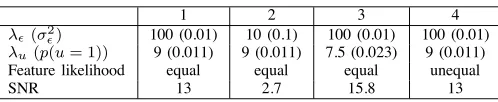
The five features used to construct all test signals are shown in figure 1. These features were chosen as the maximum cor-relation between different features is low, but the periodicity of the features means that they are strongly correlated with shifts of themselves. We generated four different test signals by drawing the non-zero coefficients from the modified Rayleigh distribution. The used parameters are listed in table I. The test signals were generated so that the first signal can be used as a reference, with the other signals varying one parameter relative to the first signal (i.e. increased noise (2), reduced sparsity (3) and reduced occurrence of feature a5 (4)).
B. Estimation of A
In applications in which the features represent physically meaningful signal structures, it is often important to compute accurate estimates of these features. We therefore evaluate the performance of the methods in terms of estimates of A. We
!0.20 0.2
!0.20 0.2
!0.20 0.2
amplitude
!0.20 0.2
5 10 15 20 25 30
!0.20 0.2
[image:7.595.314.563.284.335.2]sample
Fig. 1. Features used to generate the test signal.
TABLE I TEST SIGNAL PARAMETERS.
1 2 3 4
λ!(σ2!) 100 (0.01) 10 (0.1) 100 (0.01) 100 (0.01)
λu(p(u= 1)) 9 (0.011) 9 (0.011) 7.5 (0.023) 9 (0.011)
Feature likelihood equal equal equal unequal
SNR 13 2.7 15.8 13
here assumed that all parameters were known to the algorithm apart from the true features and sparse coefficients6.
1) Used Algorithms: We run the following four algorithms on all four data sets:
• full NN Gibbs: The algorithm that samples from A
ands with the modified Rayleigh prior on the non-zero
coefficients and uses the sample mean to estimateA;
• Grad + NN Gibbs:The gradient algorithm in which the
gradient is estimated using Gibbs sampling based on the non-negative modified Rayleigh prior;
• Grad + Gauss Gibbs: The gradient algorithm in which
the gradient is estimated using Gibbs sampling based on the Gaussian prior as previously suggested in [22];
• Grad + IS:The gradient algorithm in which the gradient
is estimated using importance sampling based on the Gaussian prior.
Note that we here vary the used algorithms and the used models individually, allowing a direct comparison between the algorithmic approaches and the models, e.g. methods (full NN Gibbs) and (Grad + NN Gibbs) only differ in the used algorithms, while methods (Grad + Gauss Gibbs) and (Grad + NN Gibbs) only differ in the used models etc.
We run the gradient methods until convergence (20 000 iterations) and used the last 10 samples out of 50 to estimate each gradient for the two Gibbs sampling methods and used 100 samples for the importance sampler. For the full Gibbs sampler we drew 1000 samples from A of which we used
the last 50 samples to estimate the mean. We initialised all algorithms using exactly the same randomly generated dictionary.
1 0.98 1 0.98 1 0.99 0.96 0.91 0.97 0.99 0.95 0.99 0.99 0.99 0.98 0.94 0.95 0.96 0.94 0.97 0.91 0.89 0.92 0.95 0.88 0.86 0.88 0.93 0.94 0.92 0.92 0.89 0.96 0.96 0.94 0.95 0.56 0.89 0.78 0.71 0.99 0.94 0.91 0.98 0.99 0.96 0.96 0.98 0.94 0.94 0.77 0.97 0.98 0.99 0.98 0.92 0.91 0.91 0.95 0.93 1 1 0.75 0.98 0.83 0.99 0.97 0.95 0.95 0.58 0.99 0.96 0.96 0.99 0.43 0.95 0.98 0.83 0.99 0.26 0.99 Average: 0.96 Average: 0.98 Average: 0.95 Average: 0.91 0.91 0.93 0.78 0.96 0.96 0.94 0.92 0.91 0.89 0.87 0.8 feature feature feature feature
Signal: 1 2 3 4
full NN Gibbs
Grad + NN Gibbs
Grad + Gauss Gibbs
[image:8.595.72.279.59.483.2]Grad + IS a1 a2 a3 a4 a5 a1 a2 a3 a4 a5 a1 a2 a3 a4 a5 a1 a2 a3 a4 a5
Fig. 2. Comparison of the accuracy of how well the different algorithms estimated the different features in the signal for the four different experimental setups used.
2) Results: In figure 2 we show the correlation between the normalised learned features and the closest true feature7.
Figure 2 shows a Hinton style diagram in which the size of each square is proportional to the measured correlation. We also summarise the results of each column using the average over the five features.
From the above results we draw the following conclusions:
• For signal one, all algorithms show roughly similar performance;
• The importance sampler performed worse on all signals;
• Increasing the noise reduced the performance of all al-gorithms, in particular the importance sampler performed significantly worse for this signal;
• Decreasing the sparsity of the test signal did decrease the
7Because !ak!2 = 1 = !ack!2, the correlation aTkack is inversely
proportional to theL2error:!ak−ack!22= 2−2a T kack.
performance of all methods;
• Features that occurred less frequent were learnt less well, in particular the gradient methods were unable to estimate these features, while the full Gibbs sampler performed best in this task;
• Comparing the gradient methods based on the Gibbs sam-pler it can be observed that using the modified Rayleigh distribution did sometimes lead to worse results than us-ing a Gaussian distribution for the non-zero coefficients; • The non-negative prior seemed to improve learning of
less frequently occurring features;
C. Estimation ofs
In this subsection we analyse the different sampling strate-gies in terms of estimation of s. Different applications use
different performance measures, for example in coding one is interested in rate-distortion, while in source separation one is interested in the distortion of the estimated sources. We therefore look at two different performance measures. First we directly compare estimates ofswith the truesvalues used
to generate the test signals. We then analyse the sparsity and reconstruction error of the approximations, i.e. the number of non-zero coefficients and the estimation error ofx.
1) Used Algorithms: To estimateswe calculated MAP
esti-mates by drawing samples using the following three sampling strategies:
• NN: The Gibbs sampler with the modified Rayleigh distribution;
• Gauss: The Gibbs sampler with the Gaussian
distribu-tion;
• IS:The importance sampling method also with the Gaus-sian distribution.
We here used signal one, the exact parameters and true dictionaryA(unless stated otherwise).
2) SNR in the Coefficient Domain: We show the signal to noise ratio for the estimates of s for the three Monte
Carlo strategies in table II. It is clear from these results that the importance sampling approach does perform significantly worse in estimating s, which should be contrasted with the
performance of this method in estimatingA, which was only
slightly worse when compared to the other approaches.
TABLE II
ESTIMATION OF S WITH THE THREE METHODS ASSUMINGAAND OTHER
PARAMETERS KNOWN.
NN Gibbs G Gibbs IS
SNR in dB (s) 43 24 -2
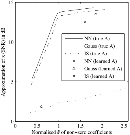
3) Sparsity vs. Reconstruction Error: To compare the algo-rithms in terms of reconstruction error and sparsity we varied the noise varianceλ−1
0 0.5 1 1.5 2 2.5 0
5 10 15
Normalised # of non!zero coefficients
Approximation of x (SNR) in dB
NN (true A) Gauss (true A) IS (true A) NN (learned A) Gauss (learned A) IS (learned A)
Fig. 3. The points show the reconstruction error and the number of non-zero coefficients using the MAP estimates ofscalculated with the three sampling
methods (NN, Gauss and IS) using the learned dictionaries. The lines show the results calculated with the true dictionary by varying the noise (λ!) and sparsity (λu) in the algorithms. Solid line: NN Gibbs; dashed line: Gauss
Gibbs; dotted line: IS.
In order to analyse how the estimation ofAinfluences the
performance in terms of reconstruction error and sparsity, we also used the learned dictionaries and the true values for λ! andλu. These results are shown as points in figure 3.
We make the following observations:
• When using the Gibbs sampler, a better estimate of A
leads to better approximations in terms of sparsity and reconstruction error;
• For a particular estimate of A we found that using the
Gibbs sampler with the modified Rayleigh prior resulted in sparser and more accurate signal approximations com-pared to the Gibbs sampler with the Gaussian prior; • The importance sampler does not produce good sparse
approximations and the variation in the results was large. • The best estimation ofs(in terms of reconstruction error and sparsity) is achieved using the prior used to generate the data.
• The Gibbs sampler outperforms the importance sampler in estimating swhen both use the same prior model.
D. Importance Sampler Performance
The reason behind the poor performance of the importance sampler in estimating s can be understood by viewing the
MAP estimation as a form of random search, where the search is distributed depending on the posterior distributions. While the Gibbs sampler draws samples from the correct distributions and frequently visits areas with high probability, the importance sampler draws the samples from a different distribution and the search is less likely to search areas with high probability.
VII. COMPARISON WITH OTHERMETHODS
In this section we compare the Monte Carlo algorithms discussed in this paper and contrast the achieved results to the results obtained with several other algorithms proposed in the literature. The main focus in this paper has been on estimation ofAand we here concentrate on this aspect.
A. Test Signal
As a test signal we use an artificial musical signal, which is motivated by our recent work on music analysis [13]. This signal was generated by using the recorded performance infor-mation of a real piano performance of Ludwig van Beethoven’s Bagatelle No. 1 Opus 33 as the sparse time-seriess(see [48]
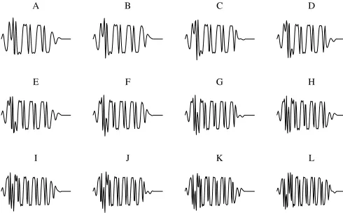
for more information on the data). To simplify the problem we restricted all pitches played to one octave and reduced the time scale. We then generated the signal using the 12 different features shown in figure 4, each 128 samples long and generated using an FM synthesis technique.
This signal is similar to the problem used in the previous subsection with the following exceptions; 1) the problem size is larger as it has more and longer features; 2) the individual features are highly correlated to features one semitone above or below (the correlation between adjacent features was between 0.5 and 0.7) and 3) the non-zero coefficients do not follow exactly the modified Rayleigh distribution. (See the histogram in figure 6 in the appendix.)
B. Used Algorithms
We here compare the following methods:
• full NN Gibbs:Sampling fromp(A,s|x)with the
mod-ified Rayleigh prior on the non-zeros;
• Grad + Gauss Gibbs: The gradient method using the
Gibbs sampler with a Gaussian prior on the non-zero s
as proposed in [22] ;
• Grad + NN Gibbs: The gradient method using the Gibbs
sampler with the non-negative modified Rayleigh prior on the non-zeros;
• Grad + IS 100 and Grad + IS 10 000: The gradient
method using the importance sampler using 100 and 10 000samples8 to estimate each gradient;
• Grad + EM: The gradient method with an estimation
of the gradient based on an approximation of p(s|x,A)
with a delta function at a local maximum [8]. We used the EM algorithm of Figueiredo [18] to find the MAP estimate. This method was previously used for the sparse approximation of time-series in [13] ;
• Grad + MP: The gradient method with an estimation
of the gradient based on Matching Pursuit. This method was previously used in [2];
• MoTIF: The MoTIF method proposed in [20], which is
a heuristic greedy learning algorithm that forces extracted featuresak to be as dissimilar as possible.
Note that method (Grad + EM) is based on an EM algorithm and requires a different model to the one used with the Monte
[image:9.595.63.288.60.293.2]A B C D
E F G H
[image:10.595.51.296.57.209.2]I J K L
Fig. 4. The twelve features used to generate the test signal.
Carlo methods whilst the Matching Pursuit and the MoTIF algorithms are not derived from any particular probabilistic formulation.
Apart from the Matching Pursuit, the MoTIF and the importance sampling methods, we used the subset selection procedure described in [13]. This method offers a fast way to select a small number of features and their associated position based on the correlation between the observed data and the features at all shifts. Similar to thresholding methods, this method calculates the correlation between the signal and all features and then selects the subset based on this correlation alone. The difference to standard thresholding methods is that selected features are not allowed to overlap with shifts of the same feature by more than a predefined amount [13]. By using this subset selection method we restrict the sampler to explore only a subset of the distribution. As it is only possible to draw a small number of samples in practice the sampler is not able to explore the distribution sufficiently even without subset selection and we found that for a fixed computational budget the performance greatly increased when combining the sampler with the subset selection method.
C. Initialisation
In all experiments we initialised the features ak with the
same set of sinusoidal functions. In table III we summarise the different parameters used for the different algorithms. The first row gives the number of features to be learned, the second row (grad iter) gives the number of iterations or samples used to evaluate each gradient and the third row shows the overall number of samples drawn from p(A|x,s) or the
number of overall gradient steps (Overall iter). Numbers in parenthesis show the actual number of samples used after the burn-in period. The fourth row contains the block size used in each iteration. The fifth row shows a rough estimate of the computation time required for each algorithm.
D. Model Parameter Estimation
The focus of this paper was on the adaptation of the features
ak. However, other model parameters can be adapted using
similar methods as studied here. In [22] maximum likelihood
gradient type update rules have been proposed and we present such updates for different model parameters in appendix V. Another possible approach would be to specify priors for all model parameters and to extend the sampler to also sample from these parameters.
The results obtained below were achieved with the model parameters learned using the gradient estimates in appendix V. However, we found that the estimation performance of the
ak did not depend strongly on the other model parameters
and experiments with parameters estimated from the true coefficientsshave produced similar results.
E. Results
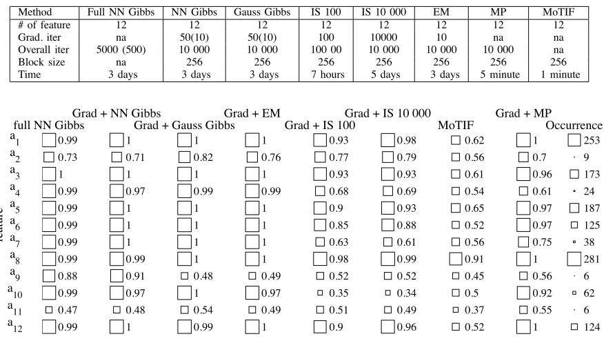
A quantitative analysis of the results is given in figure 5, where the correlations between the true features ak and the
closest learned features at the best shift are compared for the five methods. The figure shows a Hinton style diagram, where the correlation is related to the size of the squares shown. The last column in figure 5 shows the number of occurrences for each note.
We make the following observations:
• The Gibbs sampling methods outperform the other meth-ods;
• The importance sampling method did produce signifi-cantly worse results for this problem than the Gibbs sampler, which we attribute to the bias;
• Combining the subset selection procedures with the Gibbs sampling methods did perform better than the fast meth-ods;
• Again, less frequently occurring features are learned less well with all methods;
• Due to the high correlation of individual features, the features that had not been learned were often modelled quite well with features learned to represent other features and the fact that these features had not been learned did therefore not increase the overall reconstruction error significantly;
• The results obtained by sampling from A are slightly
worse than those found with the Gibbs sampling based gradient method using the same prior. This seems to be a result of the aforementioned permutation ambiguity.
VIII. CONCLUSION
TABLE III
PARAMETERS FOR THE DIFFERENT ALGORITHMS USED IN THE EXPERIMENTS.
Method Full NN Gibbs NN Gibbs Gauss Gibbs IS 100 IS 10 000 EM MP MoTIF
# of feature 12 12 12 12 12 12 12 12
Grad. iter na 50(10) 50(10) 100 10000 10 na na
Overall iter 5000 (500) 10 000 10 000 100 00 10 000 10 000 10 000 na
Block size na 256 256 256 256 256 256 256
Time 3 days 3 days 3 days 7 hours 5 days 3 days 5 minute 1 minute
0.99 0.73 1 0.99 0.99 0.99 0.99 0.99 0.88 0.99 0.47 0.99 1 0.71 1 0.97 1 1 1 0.99 0.91 0.97 0.48 1 1 0.82 1 0.99 1 1 1 1 0.48 1 0.54 0.99 1 0.76 1 0.99 1 1 1 1 0.49 0.97 0.49 1 0.93 0.77 0.93 0.68 0.9 0.85 0.63 0.98 0.52 0.35 0.51 0.9 0.98 0.79 0.93 0.69 0.93 0.88 0.61 0.99 0.52 0.34 0.49 0.96 0.62 0.56 0.61 0.54 0.65 0.52 0.56 0.91 0.45 0.5 0.37 0.52 1 0.7 0.96 0.61 0.97 0.97 0.75 1 0.56 0.92 0.55 1 253 9 173 24 187 125 38 281 6 62 6 124 full NN GibbsGrad + NN GibbsGrad + Gauss GibbsGrad + EMGrad + IS 100Grad + IS 10 000 MoTIF Grad + MPOccurrence a1 a2 a3 a4 a5 a6 a7 a8 a9 a10 a11 a12 feature
Fig. 5. Hinton style diagram showing the correlation between the learned features and the original features for the different methods. The size of the squares represents the value. The last column shows the number of occurrence of each of the features in the original signal.
The importance sampling method was faster than the Gibbs sampling based approaches. We found that for small problems this method can be used successfully to learn the features, however, for larger problems the bias introduced into the gradient estimate becomes significant and the performance was found to drop. Contrary to the performance in feature learning, the importance sampler was not able to estimate the sparse coefficientss.
Another benefit of the sampling strategies was the ability to use a range of prior distributions. We found that choosing this distribution to closely model the data offered additional performance benefits, in particular in terms of estimation of the sparse coefficientssand in terms of sparsely representing
a signal. The problem of estimating Aon the other hand was
found to be quite robust with respect to the used prior and the used parameters.
APPENDIXI
DERIVATION OFEQUATION(8)
−∂∂a k
lnp(A|x) =−
∂ ∂ak
. .
p(A,s|x)ds
. .
p(A,s|x)ds
=−
' ' p(A,s
|x)
p(A|x)
∂
∂aklnp(A,s|x)ds
=−
' '
p(s|A,x) ∂
∂ak lnp(x,A|s)ds
Because ∂∂aklnp(A,s|x) =
∂
∂aklnp(x,A|s) +
∂ ∂akln
p(s) p(x)=
∂
[image:11.595.89.527.78.325.2]∂aklnp(x,A|s).
Fig. 6. A comparison between the histogram of note velocities of a real piano performance (solid) as used in section VI and the modified Rayleigh distribution introduced in the text. Also shown are a standard Rayleigh distribution (dotted) and a shifted Rayleigh distribution (dash dotted).
APPENDIXII
THE MODIFIEDRAYLEIGHDISTRIBUTION
We define the modified Rayleigh distribution as:
pmR(s;µ,σR) =
/ 1
ZmRse−(s−µ)
2
/2σ2
mR if 0< s
0 otherwise.
(20) An example of this distribution is shown in figure 6 (dashed line). The normalising constant for this distribution is:
ZmR=σmRe−(µ)
2
/2σ2
mR+0.5µ 0
2πσ2
mR(1+erf(
µ
1
2σ2mR)),
(21) where erf(·)is the error function.
[image:11.595.92.525.79.326.2]APPENDIXIII
DERIVATION OFE1FOR THEGIBBSSAMPLER
A. Derivation of E1 forp(sn|un = 1) =pmR(s;µn,λ−R1)
If we use p(sn|un= 1) =pmR(s;µn,λ−R1), we have from
equation (17):
E1= log
p(un = 1).p(x|s,u,A)p(sn|un= 1)dsn
p(un = 0).p(x|s,u,A)p(sn|un= 0)dsn
= log
.
e−0.5λ"(x−As)T(x−As) 1
Zpsne
−0.5λR(sn−µn) 2
dsn .
e−0.5λ"(x−As)T(x−As)δ
0(sn)dsn
+ loge−0.5λu
whereZpis the normalising constant of the modified Rayleigh
distribution given in equation (21). We can write this as
E1= log
.
e−0.5λEn(bn−sn)T(bn−sn) 1 Zpsne
−0.5λR(sn−µn) 2
dsn .
e−0.5λEn(bn−sn)T(bn−sn)δ0(sn)dsn
+ loge−0.5λu
= log
1
Zp .
sne−0.5Ψns
2
n+Ψnηnsn−0.5(λEnbn2+λRµn2)ds
n
e−0.5λEn(bn)2
+ loge−0.5λu
= loge0.5λEnb
2
ne−0.5λuZE
Zp '
sne−0.5Ψn(sn−ηn)
2 dsn,
where in the last line we use
ZE=e0.5(Ψnη
2
−λE−nb 2
n−λRµ
2
n). (22)
The integral in the last line is the normalising constant in the modified Rayleigh distribution given in equation (21) so that the expression forE1 in equation (16) becomes:
E1=−
λu
2 +
λEn
2 b
2
n+ lnΦ, (23)
where
Φ= ZE Zp
2
1 Ψn
e−0.5η2Ψn+ 0.5η 3
2π
Ψn 4
1 + erf
4 η 3 Ψ 2 556 (24) with
ZE=e−0.5(−η
2 Ψn+b
2
nλEn+µ
2
nλR) (25)
and
Zp=
e−µ2n0.5λR
λR + 0.5µn 3
2π λR
7
1 + erf7µn 1
0.5λR88. (26)
ηn and Ψ1n are the parameters of the posterior p(sn|snˆ=$ n, un = 1,A), which due to the conjugate
prior is also of the modified Rayleigh form. The parameters are given analytically as:
ηn=λEnbn+λRµn
λEn+λR (27)
and
Ψn =λEn+λR (28)
Here we have used the notation λEn = λ!aTnan and bn =
(aT
nan)−1aTnx.
B. Derivation ofE1 forp(sn|un= 1)∼N(s; 0,λ−R1)
In [35] the derivation of E1 is presented for the case in
which p(sn|un = 1) = N(s; 0,λ−R1). Using the notation
introduced above forΨn and using µn= 0we get:
E1=−
λu
2 +
λEn
2 b
2
n+ 0.5 ln
2π
Ψn −
0.5λEnb2n 9
1 + λEn Ψn
:
.
(29)
APPENDIXIV
SAMPLING FROM THEMODIFIEDRAYLEIGHDISTRIBUTION
The modified Rayleigh distribution can be written as:
1 ZmR
se−(s−µ)2/2σ2mR=
1 ZmR
7
(s−µ)e−(s−µ)2/2σmR+µe−(s−µ)
2
/2σmR 8
.
This form suggests a hybrid sampling strategy. With proba-bility 1
ZmR(σmR+ 0.5µ √2
πσmR),s > µand we can sample from:
p(s|s > µ) =µ+
; σmR
ZmR <
σmR−1se−0.5σ−1
mRs
2
+
;
0.5 µ ZmR √ 2πσmR < 2 = σ−mR1
2π e
−0.5σ−1
mRs
2 ,
which is a mixture of a truncated Gaussian and a shifted Rayleigh distribution.
Fors < µwe have an upper bound on the distribution of 1
ZmR
µe−(s−µ)2/2σmR (30)
in which case rejection sampling can be used.
APPENDIXV
GRADIENTEXPRESSIONS FOR THEOTHERMODEL
PARAMETERS
Gradient expressions for other model parameters (sayθ) can be derived in a similar way to those in equation (8).
∆θ= ∂logp(A|x)
∂θ =
( ∂
∂θlogp(x,A|s) )
. (31)
Again we assume that the prior for the model parameters is relatively flat, so that the gradient of this prior is set to zero. We then get the gradient for the noise scale factorλ!
∆λ! =
(
M 2λ!−
1
2(x−As)
T(x −As)
)
, (32)
and the gradient of the parameterλu in the Bernoulli prior:
∆λu=
>
N 2(1 +eλ2u)−
1 2u
Tu ?
. (33)
For the model using a Gaussian prior for the non-zero coefficients s we get a gradient for the scale factor for the GaussianλR
∆λR=
(uTu
2λG −
1 2s
Ts )
while for the model in which the non-zero coefficientsshave
a modified Rayleigh prior we get a gradient for the modified Rayleigh parameter λR
∆λR =
>
−0.5 !
sjn$=0
(sjn−µ)2−
U c1
(−0.5µc2
λR −c3λ
−2
R ) ?
(35) and for the modified Rayleigh parameter µ
∆µ=
> !
sjn$=0
λR(sjn−µ)−
U c1
c3
?
. (36)
Here U is the number of the non-zeros, c1 =µc2+λ−R1c3,
c2 = 0.5
0
2πλ−R1(1 + erf(µ√0.5λR)) and c3 = e−0.5λRµ
2 . We also use +·, to denote the expectation with respect to p(s,u|x,A), which can again be approximated using Monte
Carlo estimates.
ACKNOWLEDGMENT
The authors would like to thank the anonymous review-ers for additional references and valuable comments, which greatly helped to improve this article.
REFERENCES
[1] V. K. Goyal, M. Vetterli, and N. T. Thao, “Quantized overcomplete ex-pansions inRN: Analysis, synthesis and algorithms,”IEEE Transactions on Information Theory, vol. 44, pp. 16–31, Jan. 1998.
[2] E. C. Smith and M. S. Lewicki, “Efficient auditory coding,” Nature, vol. 439, pp. 978–982, Feb. 2006.
[3] R. Figueras i Ventura, P. Vandergheynst, and P. Frossard, “Low rate and flexible image coding with redundant representations,”to appear in IEEE Transactions on Image Processing.
[4] M. E. Tipping, “Sparse Bayesian learning and the relevance vector machine,”Journal of Machine Learning Research, vol. 1, pp. 211–244, 2001.
[5] M. Zibulevsky and B. A. Pearlmutter, “Blind source separation by sparse decomposition in a signal dictionary,” Neural Computation, vol. 13, no. 4, pp. 863–882, 2001.
[6] M. Zibulevsky and P. Bofill, “Underdetermined blind source separa-tion using sparse representasepara-tions,”Signal Processing, vol. 81, no. 11, pp. 2353–2362, 2001.
[7] A. Hyv¨arinen, “Sparse code shrinkage: Denoising of nongaussian data by maximum likelihood estimation,” Neural Computations, vol. 11, no. 7, pp. 1739–1768, 1998.
[8] B. A. Olshausen and D. J. Field, “Emergence of simple-cell receptive field properties by learning a sparse code for natural images,”Nature, vol. 13, pp. 607–609, Jun 1996.
[9] M. S. Lewicki and B. A. Olshausen, “Infering sparse, overcomplete image codes using an efficient coding framework,” in Advances in Neural Information Processing Systems (NIPS), vol. 10, 1998. [10] A. Holobar and D. Zazula, “Correlation-based decomposition of surface
electromyograms at low contraction forces,” Medical and Biological Engineering and Computing, vol. 42, pp. 487–495, 2004.
[11] T. Blumensath and M. Davies, “Shift-invariant sparse coding for single channel blind source separation,” inProceedings of the Workshop on Signal Processing with Adaptative Sparse Structured Representations, (Rennes, France), Nov. 2005.
[12] S. Abdallah,Towards Music Perception by Redundancy Reduction and Unsupervised Learning in Probabilistic Models. PhD thesis, King’s College London, February 2003.
[13] T. Blumensath and M. Davies, “Sparse and shift-invariant representa-tions of music,” IEEE Transactions on Audio, Speech and Language Processing, vol. 14, pp. 50–57, Jan 2006.
[14] M. Plumbley, S. Abdallah, T. Blumensath, and M. Davies, “Sparse rep-resentations of polyphonic music,”ELSVIR Signal Processing, vol. 86, pp. 417–431, March 2006.
[15] G. Davis,Adaptive Nonlinear Approximations. PhD thesis, New York University, 1994.
[16] S. Mallat and Z. Zhang, “Matching pursuits with time-frequency dic-tionaries,” IEEE Transactions on Signal Processing, vol. 41, no. 12, pp. 3397–3415, 1993.
[17] S. S. Chen, D. L. Donoho, and M. A. Saunders, “Atomic decomposition by basis pursuit,”SIAM Journal of Scientific Computing, vol. 20, no. 1, pp. 33–61, 1998.
[18] M. A. T. Figueiredo, “Adaptive sparseness for supervised learning,” IEEE Transactions on Pattern Analysis and Machine Intelligence, vol. 25, pp. 1150–1159, Sept. 2003.
[19] K. Kreutz-Delgado, J. F. Murray, B. D. Rao, K. Engan, T.-W. Lee, and T. J. Sejnowski, “Dictionary learning algorithms for sparse representa-tion,”Neural Computation, vol. 15, no. 2, pp. 349–396, 2003. [20] P. Jost, P. Vandergheynst, S. Lesagne, and R. Gribonval, “MoTIF: An
efficient algorithm for learning translation invariant dictionaries,” in Proc. of the Int. Conf. on Accoustic, Speech and Signal Processing, May 2006.
[21] B. A. Olshausen and K. Millman, “Learning sparse codes with a mixture-of-gaussians prior,” in Advances in Neural Information Processing Systems (NIPS), pp. 841–847, 2000.
[22] P. Sallee and B. A. Olshausen, “Learning sparse multiscale image representations,” inAdvances in Neural Information Processing Systems (NIPS), pp. 1327–1334, 2003.
[23] T. Blumensath and M. Davies, “Enforcing sparsity, shift-invariance and positivity in a Bayesian model of polyphonic music,” inProc. of the IEEE Workshop on Statistical Signal Processing, July 2005.
[24] T. Blumensath and M. Davies, “A fast importance sampling algorithm for unsupervised learning of over-complete dictionaries,” inProc. of the Int. Conf. on Acoustics, Speech and Signal Processing, pp. 213–216, March 2005.
[25] M. S. Lewicki and T. J. Sejnowski, “Coding time-varying signals using sparse, shift-invariant representations,” in Advances in Neural Information Processing Systems (NIPS), vol. 11, pp. 730–736, 1999. [26] R. Bogacz, M. W. Brown, and C. Giraud-Carrier, “Emergence of
movement-sensitive neurons’ properties by learning a sparse code of natural moving images,” inAdvances in Neural Information Processing Systems (NIPS), pp. 838–844, 1999.
[27] B. A. Olshausen, “Sparse coding of time-varying natural images,” in Proc. of the Int. Conf. on Independent Component Analysis and Blind Source Separation, 2000.
[28] H. Wersing, J. Eggert, and E. K¨orner, “Sparse coding with invariance constraints,” in Proc. Int. Conf. Artificial Neural Networks ICANN, pp. 385–392, 2003.
[29] E. Smith and M. S. Lewicki, “Efficient coding of time-relative structure using spikes,”Neural Computation, vol. 17, pp. 19–45, Jan 2005. [30] C. P. Robert and G. Casella,Monte Carlo Statistical Methods. Springer
Texts in Statistics, Springer-Verlag, 1999.
[31] A. Hyv¨arinen, J. Karhunen, and E. Oja,Independent Component Anal-ysis. John Wiley & Sons Inc, 2001.
[32] M. Girolami, “A variational method for learning sparse and overcomplete representations,”Neural Computaion, vol. 11, pp. 2517 – 2532, 2001. [33] C. Fevotte and S. Godsill, “A bayesian approach for blind separation of
sparse sources,” IEEE Transactions on Speech and Audio Processing, vol. PP, no. 99, pp. 1–15, 2005.
[34] M. S. Lewicki and T. J. Sejnowski, “Learning overcomplete representa-tions,”Neural Computation, no. 12, pp. 337–365, 2000.
[35] J. Geweke, “Variable selection and model comparison in regression,” in Bayesian Statistics 5.(J. M. Bernardo, J. O. Berger, A. P. Dawid, and A. F. M. Smith, eds.), Oxford University Press, 1996.
[36] K. Kreutzer-Delgado, B. D. Rao, and K. Engan, “Convex/ Schur-Convex (CSC) log-priors and sparse coding,” inProc. of the 6th Joint Symposium on Neural Computation, (Pasadena, California), May 1999.
[37] H. J. Kushner and G. G. Yin,Stochastic Approximation and Recursive Algorithms and Applications. Springer-Verlag New York, 2003. [38] G. Celeux, M. Hurn, and C. P. Robert, “Computational and inferential
difficulties with mixture posterior distributions,” J. American Statist. Assoc., vol. 9, no. 3, pp. 957–979, 2000.
[39] M. Stephens, “Dealing with label-switching in mixture models,”Journal of the Royal Statistical Society, Series B, vol. 62, pp. 795–809, 2000. [40] M. S. Lewicki and B. A. Olshausen, “A probabilistic framework for the
adaptation and comparison of image codes,”J. Opt. Soc. Am. A: Optics, Image Science, and Vision, vol. 16, no. 7, pp. 1587–1601, 1999. [41] M. Smith and R. Kohn, “Nonparametric regression using Bayesian
variable selection,”Journal of Econometrics, vol. 75, no. 2, pp. 317–343, 1996.
[43] R. E. McCulloch and E. I. George, “Approaches for Bayesian variable selection,”Statistica Sinica, vol. 7, no. 2, pp. 339–374, 1997. [44] C. Han and B. P. Carlin, “Markov chain Monte Carlo methods for
com-puting Bayes factors: A comparative review,”Journal of the American Statistical Association, vol. 96, no. 455, pp. 1122–1134, 2001. [45] C. Andrieu, P. Djuric, and A. Doucet, “Model selection by MCMC
computation,” Signal Processing, Special Issue on MCMC for Signal Processing, vol. 81, no. 1, pp. 19–37, 2001.
[46] C. F´evotte and S. J. Godsill, “Sparse linear regression in unions of bases via Bayesian variable selection,”IEEE Signal Processing Letters, vol. 13, pp. 441–444, Jul. 2006.
[47] R. E. McCulloch and E. I. George, “Variable selection via Gibbs sampling,” Journal of the American Statistical Association, pp. 881– 889., September 1993.
[48] J. P. Bello,Towards the Automated Analysis of Simple Polyphonic Music: A Knowledge-based Approach. PhD thesis, Queen Mary, University of London, 2003.
PLACE PHOTO HERE
Thomas Blumensathreceived the BSc hons. degree in music technology from Derby University, Derby, U.K., in 2002 and his Ph.D. degree in electronic engineering from Queen Mary, University of Lon-don, U.K., in 2006. He is currently a postdoctoral research fellow in the Institute for Digital Commu-nication at the University of Edinburgh, working on sparse representations for signal processing and coding. His research interests include mathematical and Bayesian methods in signal processing, unsu-pervised learning, sparse signal approximations and applications to music and audio analysis.
PLACE PHOTO HERE