On Long Term Climate Studies Using a Coupled General Circulation Model

Experimental design

A.1

Introduction

The experimental design employed throughout this project followed that specified by PMIP2 (Paleoclimate Modelling Intercomparison Project, 2005), enabling a direct comparison between Mk3L and other models. PMIP2 experimental design is sum-marised in Section A.2, while Sections A.3 and A.4 provide further details regarding spin-up procedures and the coupled model experiments respectively.

The procedures followed to generate the restart and auxiliary files required by Mk3L are described in detail by Phipps (2006).

A.2

PMIP2 experimental design

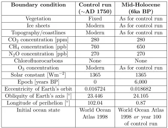
PMIP2 experimental design is summarised in Table A.1. For coupled model ex-periments, it is specified that a control run be conducted for pre-industrial con-ditions, which are taken as being those which existed around the year AD 1750. Pre-industrial values are specified for the atmospheric concentrations of the “green-house gases” carbon dioxide (CO2), methane (CH4) and nitrous oxide (N2O); it is

also specified that the atmospheric concentration of chlorofluorocarbons be set to zero. The specified epoch is 0 years Before Present, and the values for the Earth’s orbital parameters therefore correspond to the year AD 1950. Otherwise, “mod-ern” boundary conditions are specified, which can be interpreted as meaning that present-day values should be used.

While no specific spin-up procedure is prescribed for the coupled model, it is specified that the ocean model should be initialised using the World Ocean Atlas 1998 dataset (National Oceanographic Data Center, 2002, commonly referred to as the “Levitus 1998” dataset).

The boundary conditions for the mid-Holocene experiment differ only in the atmospheric methane concentration and the values of the Earth’s orbital parameters. While the ocean model can again be initialised using the World Ocean Atlas 1998 dataset, it can also be initialised from year 100 of a control run.

Boundary condition Control run Mid-Holocene

(_∼AD 1750) (6ka BP)

Vegetation Fixed As for control run Ice sheets Modern As for control run Topography/coastlines Modern As for control run CO2 concentration [ppm] 280 280

CH4 concentration [ppb] 760 650

N2O concentration [ppb] 270 270

Chlorofluorocarbons None None O3 concentration Modern As for control run

Solar constant [Wm−2_{] 1365 1365}

Epoch [years BP] 0 6,000

Eccentricity of Earth’s orbit 0.016724 0.018682 Obliquity of Earth’s axis [◦_{] 23.446 24.105}

Longitude of perihelion [◦_{] 102.04 0.87}

Initial ocean state World Ocean World Ocean Atlas Atlas 1998 1998 or year 100

of control run

Table A.1: PMIP2 experimental design for coupled model experiments: the pre-industrial control run, and the mid-Holocene experiment.

A.3

Spin-up procedures

The spin-up procedures for the atmosphere and ocean models are outlined in Sec-tions 2.3.1 and 2.3.2 respectively. This section provides further information regard-ing the experimental design.

A.3.1 Ocean model

Configuration

The default configuration of the ocean model was employed, as described byPhipps (2006). Following PMIP2 experimental design, the bathymetry and coastlines were configured for the present day.

Initial state

The initial state of the ocean model was one in which the ocean is at rest. Following PMIP2 experimental design, the initial temperatures and salinities were set equal to the annual-mean World Ocean Atlas 1998 values.

Boundary conditions

As the upper layer of the Mk3L ocean model has a thickness of 25 m, the tem-perature and salinity of this layer simulate the average temtem-perature and salinity of the upper 25 m of the water column, and not the sea surface temperature (SST) and sea surface salinity (SSS) per se. The temperature and salinity of this layer should be relaxed towards an equivalent observational quantity; the surface boundary con-ditions on the ocean model werenot therefore the observed SST and SSS, but were instead the averages of the World Ocean Atlas 1998 temperatures and salinities over the upper 25 m of the water column.

The surface wind stresses were taken from the NCEP-DOE Reanalysis 2, and consisted of the climatological wind stresses for the period 1979–2003.

A.3.2 Atmosphere model

Configuration

The default configuration of the atmosphere model was employed, as described by Phipps (2006). Following PMIP2 experimental design, the topography, coastlines, ice sheets and vegetation were configured for the present day. The solar constant was set to 1365 Wm−2_{, and AD 1950 values were used for the Earth’s orbital}

parameters. The atmospheric carbon dioxide concentration was set to 280 ppm, and ozone concentrations were taken from the AMIP II recommended dataset (Wang et al., 1995).

PMIP2 experimental design also specifies the atmospheric concentrations of methane, nitrous oxide and chlorofluorocarbons; however, the Mk3L atmosphere model does not allow for the radiative effects of these gases.

Initial state

The atmosphere model was initialised using the original restart file, as supplied with the model source code.

Boundary conditions

For consistency with the ocean model, the surface boundary conditions on the stand-alone atmosphere model consisted of the averages of the World Ocean Atlas 1998 temperature and salinity over the upper 25 m of the water column.

The currents required by the sea ice model were diagnosed from the final 100 years of ocean model spin-up runs, avoiding any need to apply “flux” adjust-ments to the currents within the coupled model.

A.4

Coupled model

A.4.1 Control runs

Configuration

surface fluxes, sea surface temperatures and sea surface salinities diagnosed from the spin-up runs, as described in Section 2.6.

Initial state

The atmospheric and oceanic components of the coupled model were initialised from the state of each model at the end of the appropriate spin-up run.

A.4.2 Mid-Holocene experiments

Configuration

For the mid-Holocene experiments, only two changes were made to the configuration of the coupled model, relative to the control runs. Following PMIP2 experimental design, the epoch was changed from 0 to 6,000 years BP. The atmospheric carbon dioxide concentration was also reduced to 277 ppm, in order to represent the ra-diative forcing arising from the specified reduction in the methane concentration (Table A.1).

This effective carbon dioxide concentration was calculated using the following expressions, which give the radiative forcings arising from changes in the atmospheric concentrations of carbon dioxide and methane (Ramaswamy et al., 2001, Table 6.2):

CO2: ∆F = 5.35 ln

C C0

(A.1)

CH4: ∆F = 0.036(

√

M ₋√M0)₋(f(M, N0)₋f(M0, N0)) (A.2)

In these expressions, ∆F is the radiative forcing (Wm−2_{), C0 and C are the}

original and perturbed carbon dioxide concentrations respectively (ppm), M0 and

M are the original and perturbed methane concentrations respectively (ppb),N0 is

the nitrous oxide concentration (ppb), and f(M, N) is given by

F(M, N) = 0.47 lnh1 + 2.01_×10−5_{(M N)}0.75_{+ 5.31}

×10−15M(M N)1.52

i

(A.3)

UsingM0 = 760 ppb,M = 650 ppb andN0 = 270 ppb, Equations A.2 and A.3

give a value of -0.066 Wm−2 _{for the radiative forcing arising from the reduction in}

the atmospheric methane concentration.

By re-arranging Equation A.1, the following expression is obtained, enabling an effectivecarbon dioxide concentrationCto be derived, which gives rise to a radiative forcing ∆F (Wm−2_{) relative to theactual concentration C0:}

C =C0e∆F/5.35 (A.4)

UsingC0 = 280 ppm and ∆F = -0.066 Wm−2, this expression gives a value for

the effective carbon dioxide concentration of 277 ppm.

Initial state

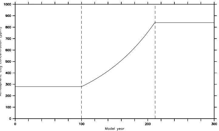
Figure A.1: The atmospheric carbon dioxide concentration for the 3_×CO2

stabili-sation experiments. After being held constant at the pre-industrial concentration of 280 ppm for the first 100 years, the carbon dioxide concentration was increased at 1% per year, until it reached 840 ppm (three times the pre-industrial concentration) in year 211. It was held constant thereafter.

A.4.3 3_×CO2 stabilisation experiments

Configuration

For the 3_×CO2 stabilisation experiments, the only change to the configuration of

the coupled model, relative to the control runs, was an increase in the atmospheric carbon dioxide concentration. The experiments began in year 101, with the carbon dioxide concentration being increased at 1% per year. It reached 840 ppm, three times the pre-industrial level, in year 211, and was held constant thereafter. The resulting carbon dioxide concentrations are shown in Figure A.1.

Initial state

Details of simulations

The simulations presented herein were conducted primarily at the Australian Part-nership for Advanced Computing National Facility (Australian Partnership for Ad-vanced Computing, 2005) in Canberra. Two different machines were used:

AlphaServer SC 126 Compaq AlphaServer SC nodes, each containing: - 4_×1GHz EV68 (Alpha 21264C) CPUs

- between 4 and 16GB of RAM Tru64 UNIX operating system

Linux Cluster 152 Dell Precision 350 nodes, each containing: - 1 _×2.66GHz Intel Pentium 4 CPU

- 1GB RAM

Linux operating system

Some of the simulations conducted on the AlphaServer SC were completed on an equivalent facility located at the Interactive Virtual Environments Centre in Perth, Western Australia.

Statistics are provided in Tables B.1, B.2 and B.3, for the atmosphere model, ocean model and coupled model simulations respectively.

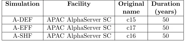
Simulation Facility Original Duration

name (years)

A-DEF APAC AlphaServer SC c15 50 A-EFF APAC AlphaServer SC c17 50 A-SHF APAC AlphaServer SC c16 50

Table B.1: Atmosphere model simulations: the name used herein, the facility on which it was conducted, the name used on that facility, and the duration.

Simulation Facility Original Duration

name (years)

O-5d APAC Linux Cluster h73 4500 O-7.5d APAC Linux Cluster h74 3500 O-10d APAC Linux Cluster h69 3500 O-15d APAC Linux Cluster h70 4500 O-30d APAC Linux Cluster h71 5500 O-40d APAC Linux Cluster h72 5500 O-60d APAC Linux Cluster h75 5500 O-80d APAC Linux Cluster h76 6500 O-0.25psu APAC Linux Cluster h57 4500 O-0.5psu APAC Linux Cluster h56 4500 O-1psu APAC Linux Cluster h55 4500 O-DEF APAC Linux Cluster h53 4500 O-EFF APAC Linux Cluster h65 8600 O-SHF APAC Linux Cluster h61 500

Table B.2: Ocean model simulations: the name used herein, the facility on which it was conducted, the name used on that facility, and the duration.

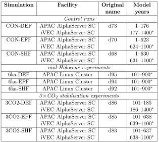
Simulation Facility Original Model

name years

Control runs

CON-DEF APAC AlphaServer SC d73 1–176 iVEC AlphaServer SC 177–1400∗

CON-EFF APAC AlphaServer SC d70 1–623 iVEC AlphaServer SC 624–1100∗

CON-SHF APAC AlphaServer SC d68 1–630 iVEC AlphaServer SC 631–1100∗

mid-Holocene experiments

6ka-DEF APAC Linux Cluster d95 101–900∗

6ka-EFF APAC Linux Cluster d94 101–900∗

6ka-SHF APAC Linux Cluster d92 101–900∗

3_×CO2 stabilisation experiments

3CO2-DEF APAC AlphaServer SC d86 101–185 iVEC AlphaServer SC 186–1400∗

3CO2-EFF APAC AlphaServer SC d85 101–638 iVEC AlphaServer SC 639–1100∗

3CO2-SHF APAC AlphaServer SC d83 101–637 iVEC AlphaServer SC 638–1100∗

Table B.3: Coupled model simulations: the name used herein, the facility on which it was conducted, the name used on that facility, and the model years which were conducted on that facility. The mid-Holocene and 3_×CO2 stabilisation experiments