Studies into the detection of buried objects (particularly optical fibres) in saturated sediment Part 2: design and commissioning of test tank

Studies into the Detection of Buried Objects (Particularly Optical Fibres) in Saturated Sediment. Part 2: Design and

Commissioning of Test Tank

T.G. Leighton and R.C.P. Evans

SCIENTIFIC PUBLICATIONS BY THE ISVR

Technical Reports are published to promote timely dissemination of research results by ISVR personnel. This medium permits more detailed presentation than is usually acceptable for scientific journals. Responsibility for both the content and any opinions expressed rests entirely with the author(s).

Technical Memoranda are produced to enable the early or preliminary release of information by ISVR personnel where such release is deemed to the appropriate. Information contained in these memoranda may be incomplete, or form part of a continuing programme; this should be borne in mind when using or quoting from these documents.

Contract Reports are produced to record the results of scientific work carried out for sponsors, under contract. The ISVR treats these reports as confidential to sponsors and does not make them available for general circulation. Individual sponsors may, however, authorize subsequent release of the material.

COPYRIGHT NOTICE

(c) ISVR University of Southampton All rights reserved.

Studies into the detection of buried objects (particularly optical fibres) in saturated sediment. Part 2: Design and commissioning of test tank

T G Leighton and R C P Evans

UNIVERSITY OF SOUTHAMPTON

INSTITUTE OF SOUND AND VIBRATION RESEARCH FLUID DYNAMICS AND ACOUSTICS GROUP

Studies into the detection of buried objects (particularly optical fibres) in saturated sediment. Part 2: Design and commissioning of test tank

by

T G Leighton and R C P Evans

ISVR Technical Report No. 310

April 2007

Authorized for issue by

Professor R J Astley, Group Chairman

ACKNOWLEDGEMENTS

TGL is grateful to the Engineering and Physical Sciences Research Council and Cable & Wireless for providing a studentship for RCPE to conduct this project.

CONTENTS

ACKNOWLEDGEMENTS ii

CONTENTS iii

FIGURE CAPTIONS v

ABSTRACT ix

LIST OF SYMBOLS xi

1 INTRODUCTION 1

2 THE TEST FACILITY 2

2.1 The Sediment Bed 2

2.1.1 Bubble Entrainment 4

2.1.2 Particle Size Distribution 7

2.2 Sound Speed and Attenuation 9

2.2.1 Sound Speed 9

2.2.2 The Attenuation of Sound in Seawater 13 2.2.3 The Attenuation of Sound in Suspensions 14

2.2.4 The Attenuation of Sound in the Seabed 17 2.2.5 The Seawater-Seabed Interface 23

2.3 Summary of design considerations for sediment tank 25

3 TRANSDUCER DESIGN 27

3.1 The Design of an Acoustic Reflector 29 3.2 Free-Field Characterisation 33

3.3 Transmission Loss 35

4 THE AUTOMATED CONTROL SYSTEM 38

5 SUMMARY 41

A.1 CALCULATION OF THE PARAXIAL FOCUS 44

A.3 MODELLING THE CAUSTIC 48

FIGURE CAPTIONS

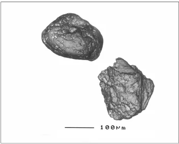
Figure 1 A scanning electron microscope picture of two typical sand

grains taken from the sediment bed. The scale bar is 100 µm in length.

3

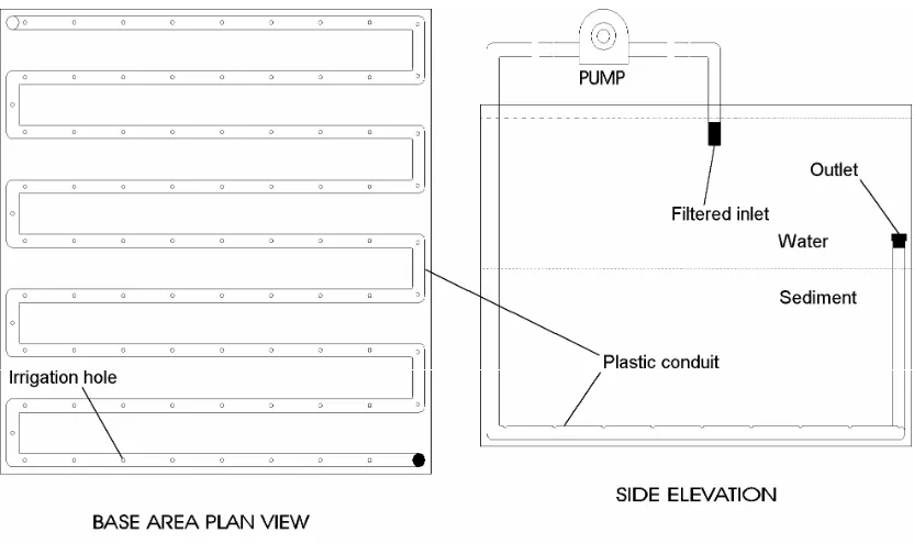
Figure 2 Schematic layout of the fluidisation system. Bubbles were

removed from the sediment by a stream of water, pumped into the conduit

and expelled through the irrigation holes.

6

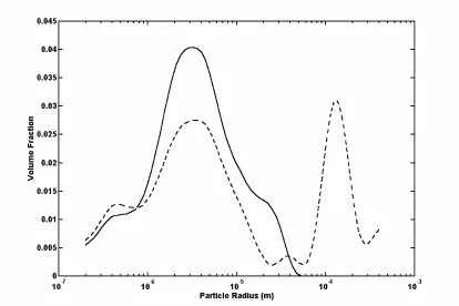
Figure 3 The measured size distributions of sand particles in a light

suspension (solid curve) and from a few centimetres beneath the surface of

the sediment in the laboratory tank (dashed curve).

8

Figure 4 The typical sound speed profile observed in the deep ocean7

[20].

10

Figure 5 Side view of the source / receiver arrangement for the speed of

sound measurements in water and water-saturated sediment in the

laboratory tank.

12

Figure 6 The absorption coefficient in seawater according to the

expression of Fisher and Simmons [29] in Lyman and Fleming seawater

[30] of salinity 3.5 % and pH = 8.0. The thick solid line is the combined

absorption for pure water and the ionic compounds, magnesium sulphate

and boric acid.

14

function of acoustic frequency and particle radius for a suspension of

spherical quartz particles with a mass concentration of 0.2 kg m-3 [36].

(Original in colour.)

Figure 8 The attenuation coefficient calculated for a suspension of sand

particles in the laboratory tank with a mass concentration of 0.2 kg m-3.

17

Figure 9 The attenuation coefficient measured in a range of naturally

occurring, saturated marine sediments [2, 25, 45]. Symbols: × = sands, all

grades; + = sand-silt, silt-sand, sand-silt-clay; • = clay-silt, silt, silt-clay;

and 6 = various clays. The straight line corresponds to an attenuation

coefficient of α_dB =0 5. f_k1. (Original in colour.)

19

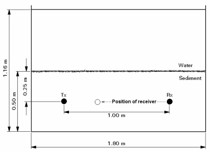
Figure 10 Side view of the source / receiver arrangement for the sediment

attenuation measurement in the laboratory tank. The filled symbols

represent the initial positions of the acoustic source, Tx, and receiver, Rx.

The outlined symbol represents the range of positions of the receiver.

20

Figure 11 The average attenuation coefficient measured in the laboratory

sand is marked by the curve. The error bars at selected frequencies

correspond to a standard deviation of ± 1. A subset of the historical data

(see figure 9) for a range of sandy sediments are marked by the points, ×.

The straight line corresponds to an attenuation coefficient of αdB=0 5fk 1

. .

23

Table 1 Simulation results for 25, 30 and 35 cm diameter spherical reflectors.

Figure 12 The design specification for an acoustic reflector. 32

Figure 13 The sound field generated by a focused acoustic reflector

(focusing at ∞). The crosses represent discrete measurement positions and

the solid line delineates the theoretical boundary of the acoustic field.

(Original in colour.)

34

Figure 14 The source / receiver arrangement for the sediment transmission loss measurement in the laboratory tank. The filled symbols

represent the initial positions of the acoustic source, Tx, and receiver, Rx.

The outlined symbols represent the range of positions of Tx and Rx.

36

Figure 15 The sound field generated within the sediment bed by a focused

acoustic reflector. The crosses represent discrete measurement positions.

The solid line indicates the calculated position of the acoustic axis.

(Original in colour.)

37

Figure 16 The position control rig mounted above the laboratory tank. 39

Figure 17 The arrangement of the signal generation / data acquisition

hardware that was used in the laboratory tank automated control system.

40

Figure 18 An example scanning pattern for the automated position control

system, as viewed from the side of the laboratory tank. Symbols:

+ = discrete positions of the acoustic projector; × = discrete positions of

the acoustic receiver; ο = points of intersection within the sediment.

Table 2 A summary of the parameters identified in this report. 42

Figure A 1 An acoustic source and a section of a spherical reflector. The

path of a marginal ray from the source, S0, to the axial-intercept, Si, is

shown.

44

Figure A 2 The longitudinal and transverse spherical aberrations

associated with a spherical reflector.

47

Figure A 3 A ray-traced caustic illustrating the circle of least confusion,

ΣLC.

ABSTRACT

This report is the second in a series of five, designed to investigate the detection of targets buried in saturated sediment, primarily through acoustical or acoustics-related methods. Although steel targets are included for comparison, the major interest is in targets (polyethylene cylinders and optical fibres) which have a poor acoustic impedance mismatch with the host sediment. This particular report details the construction of a laboratory-scale test facility. This consisted of three main components. Budget constraints were an over-riding consideration in the design.

First, there is the design and production of a tank containing saturated sediment. It was the intention that the physical and acoustical properties of the laboratory system should be similar to those found in a real seafloor environment. Particular consideration is given to those features of the test system which might affect the acoustic performance, such as reverberation, the presence of gas bubbles in the sediment, or a suspension of particles above it. Sound speed and attenuation were identified as being critical parameters, requiring particular attention. Hence, these were investigated separately for each component of the acoustic path.

Second, there is the design and production of a transducer system. It was the intention that this would be suitable for an investigation into the non-invasive acoustic detection of buried objects. A focused reflector is considered to be the most cost-effective way of achieving a high acoustic power and narrow beamwidth. A comparison of different reflector sizes suggested that a larger aperture would result in less spherical aberration, thus producing a more uniform sound field. Diffraction effects are reduced by specifying a tolerance of much less than an acoustic wavelength over the reflector surface. The free-field performance of the transducers was found to be in agreement with the model prediction. Several parameters have been determined in this report that pertain to the acoustical characteristics of the water and sediment in the laboratory tank in the 10 – 100 kHz frequency range.

Third, there is the design and production of an automated control system was developed to simplify the data acquisition process. This was, primarily, a motor-driven position control system which allowed the transducers to be accurately positioned in the two-dimensional plane above the sediment. Thus, it was possible for the combined signal generation, data acquisition and position control process to be co-ordinated from a central computer.

difficult targets (including centimetre-scale plastic objects and optical fibres) buried in saturated sediment” by T G Leighton and R C P Evans, written for a Special Issue

of Applied Acoustics which contains articles on the topic of the detection of objects

LIST OF SYMBOLS

A A constant describing the amplitude of the scaler potential of a transmitted wave

anp Attenuation coefficient

B A constant describing the decay in amplitude of the scaler potential of a transmitted wave

cf Speed of sound in a fluid

c1 Phase speed of compressional acoustic waves in medium 1 c2 Phase speed of compressional acoustic waves in medium 2

e Exponential constant (~2.71828182)

fk Acoustic frequency in kilohertz Fr Paraxial focal length

H(ω) Frequency-domain transfer function

IL Intensity level

Ipa Pulse averaged acoustic intensity Iref Reference acoustic intensity

j _{Complex operator, −1}

Kb Complex bulk modulus of a sediment’s skeletal frame

ki Wave number of an incident wave

kα An empirical constant describing the frequency dependence of

attenuation.

Li Distance from Si to the rim of a spherical reflector LSA Longitudinal spherical aberration

n An integer, in this report for example denoting the number of equations, or estimates

nα An empirical constant describing the frequency dependence of

attenuation.

O Reference position of the back of a spherical reflector OPL Optical path length

Patm Atmospheric pressure

Pe Effective acoustic pressure amplitude

Pg Gauge pressure

Pref Reference effective acoustic pressure amplitude

RPa Pressure amplitude reflection coefficient rr Radius of the aperture of a spherical reflector

Rr The principal radius of curvature of a spherical reflector Rπ Power reflection coefficient

S0 Separation between acoustic elements or between an acoustic element and the back of a spherical reflector (point O in figure A 1)

Si Distance between the point of intercept of a ray on the acoustic axis and the back of a spherical reflector (point O in figure A 1)

S(ω) Signal input to a signal processor (excluding noise)

t Time T Temperature (°C)

tg Gauge temperature (T / 100)

TPa Pressure amplitude transmission coefficient TSA Transverse spherical aberration

x Cartesian co-ordinate in the horizontal plane, used in this report for example to describe the distance between two hydrophones which lie in the same horizontal plane, or the horizontal coordinate direction along the interface between two media.

xr Depth of the aperture of a spherical reflector x1 Horizontal co-ordinate of measurement position 1 x2 Horizontal co-ordinate of measurement position 2 X(ω) Frequency response of a detection system

z The vertical Cartesian co-ordinate, in this report reflecting the penetration depth of a wave into a medium

Z Characteristic acoustic impedance

Z1 Characteristic acoustic impedance of medium 1 Z2 Characteristic acoustic impedance of medium 2

αdB Attenuation coefficient

∆ Directivity function

φr Complementary angle, φ_r =

(

)

ϕr Angle subtended between the rim and the back of a spherical reflector

π Pi (≈ 3.141592654)

θc Critical angle

θg Grazing angle

θi Angle of incidence

θr the angle measured at the sound source and subtended between the rim of a spherical reflector and the acoustic axis

ρf Density of a fluid

ΣLC Diameter of the circle of least confusion

ς ς =(R_r −S₀)/L₀ is a constant for a given spherical reflector

ω Circular frequency

ψ Acoustic wave potential

ψi Incident scaler acoustic wave potential

ψr Reflected scalar wave potential

ψt Transmitted scalar wave potential

ψx Tangential scalar wave potential along an interface (in the x-direction)

1 Introduction

In the previous report1, a system based on acoustic techniques was identified as being the most likely to succeed in the direct detection of buried objects. In order to investigate this, experimentally, it was necessary to build a test facility to mimic the seabed environment. In this report, the design and construction of such a facility is described.

In the next section of this report (section 2), the physical and acoustical properties of the seabed environment are studied individually. In particular, the size and shape of the sediment material used in the test facility is examined, as well as the speed of sound and attenuation in seawater, sediment suspensions, and within the sediment. In the sub-sections that follow, these properties are compared to those found in the laboratory.

It should be noted that the acoustic path length in a field system is estimated to be up to 2 m through the water, and up to 2 m in the sediment (for the round-trip, from an ROV-mounted transducer to an object buried at a depth of up to 1 m in the sediment, and back again). A system of this size was impractical to build in the laboratory with the facilities available. Therefore, an important goal of this section was to ensure that a scaled-down version of the field environment would still give useful results.

The third section of this report deals with the transducer system. This was designed to reduce unwanted acoustic interaction with the environment, whilst increasing the likelihood of interaction with a buried object. Measurements are presented for both the free-field performance of the system, and the transmission loss within the sediment.

Section 4 briefly details the position control system which guided the transducers within the tank. Under the direction of a single computer, the laboratory apparatus formed a completely automated signal generation, data acquisition and position control system.

1

2

The Test Facility

A large steel tank (150 cm × 180 cm × 125 cm deep) was obtained for the purpose of creating an acoustic test facility. It was mounted on a series of wooden blocks to reduce vibration-induced background noise. The tank was part-filled with a sediment-like material to a depth of 50 cm, and water to give a total fill-depth of 116 cm. The physical nature of the sediment and the acoustic behaviour of the water and sediment media are considered in the next two sections. Important properties are summarised in section 2.3, and the implications for the design of an acoustic detection system are discussed.

2.1 The Sediment Bed

At a sea depth of 1 000 m the seabed is, typically, composed of fine sand and clay-silt, with a mean particle diameter of less than 100 microns [1]. To reproduce ‘at-sea’ acoustic conditions in the laboratory tank, it was important to ensure that the composition of the artificial sediment was similar to a real seabed. A favoured laboratory material is round-grained quartz sand, which has less rigidity and attenuation than angular-grained natural sands [2]. Alternatives such as spherical particles were also considered [3] but were found to be too expensive to be used in large quantities.

For the large quantity of sediment that was required, the most convenient and cost-effective material was found to be ordinary builder’s sand. The sand used conformed to the British Standard, BS 1200; a standard that specifies the process of sieving which controls the particle size distribution. (The distribution of sand grains was subsequently measured directly using a laser light scattering technique. This is presented in detail in section 2.1.2).

to minimise the number of air bubbles trapped within the sediment. Details of the preventative measures that were taken are presented in section 2.1.1.

In total, 2400 kg of sand was stirred into the laboratory tank, already half-filled with tap water, to achieve a fill-depth of 50 cm. The density of a sample of individual sand grains was measured to be 2 670 kg m-3 ± 2.5 %. (For convenience, the commonly accepted value of 2 650 kg m-3, the density of quartz [5], was used in calculations.) The density of water was taken to be 1 000 kg m-3 with an uncertainty of ± 0.1 %, arising mainly through temperature variations. From these values, the bulk density of the water-saturated sediment was calculated to be 2 110 kg m-3± 2.5 %. (The porosity was also calculated using these values and was found to be, roughly, 0.33. This is typical of the porosities measured in sediments of this type [6].)

Figure 1 A scanning electron microscope picture of two typical sand grains taken

A scanning electron microscope2 (SEM) image of some typical sand particles is presented in figure 1. The SEM was able to resolve surface topography to within 3.5 nm and could perform microanalysis and element distribution mapping with a spatial resolution of around 5 nm. Microanalysis showed the particles to be principally composed of silicon and oxygen, as expected. The angular surface features on the grains should be noted. These crevices are ideally suited for trapping pockets of air and can act as nucleation points for the generation of bubbles which may then pass into the body of the sediment [7].

2.1.1 Bubble Entrainment

Perhaps the greatest single problem with experiments involving water-saturated sediments comes from the entrainment of bubbles [2]. Gas bubbles do not present a problem at a sea depth of 1 000 m as the rate of biological out-gassing is very low. The deposition rate of silt from dead organic matter, plankton, etc., is between 0.1 mm and 10 mm every 1 000 years [8]. In the laboratory, however, the inclusion of bubbles is inevitable.

Consider the dry sand which was added to the water in the laboratory tank. It has been noted that irregularities on the surfaces of individual sand grains could have trapped pockets of air that would have formed bubbles. By allowing the sediment to settle out, some bubbles would have detached themselves naturally. However, without active removal, a population of bubbles would have remained and, under the influence of diurnal temperature variations, even more bubbles would have formed [7].

Several methods of bubble removal were considered. These included: the initial entrainment of less air by using smooth, spherical particles [3]; the evacuation of air from the sediment by using a vacuum chamber [4]; and the acquisition of real, bubble-free sediment. Each of the above methods was excluded for reasons of cost or difficulty of implementation. An alternative method, the removal of bubbles by fluidising the sediment (i.e., by directly agitating the sand grains) was chosen as the most practical and economical solution.

2

The principle of a ‘fluidised bed’ [9] is well understood and such systems have been used in the chemical industry for a long time. If a granular material is poured into a container the surface becomes inclined at the angle of pouring. This is referred to as a ‘fixed bed’ [9]. If a fluid stream, gas or liquid, is passed upwards through the bed at a sufficient velocity, such that the force resisting the flow is equal to the bed weight, it becomes suspended and expands. Adjacent particles become mobile and the surface levels itself like a fluid. It is for this reason that the bed is said to be fluidised.

For the purpose of removing bubbles from the experimental apparatus, a fully fluidised bed was not thought to be required and, given the large volume of sediment, was not really feasible. A constant stream of water passing through the fixed sediment bed at a speed below the limit of stability, which marks the transition to the fluidised state, was expected to provide sufficient agitation to remove bubbles.

Unfortunately, there is no simple method of determining the quantities of gas bubbles present in saturated sediment and, therefore, no reliable means of gauging the effectiveness of this approach [10]. However, the results presented in later sections prove that the effect of any bubbles that may have been present was insignificant3. The layout of the fluidisation system within the laboratory tank is shown in figure 2. A small water pump (44 m head, 40 _l / minute peak flow rate) was used to force a stream of water up through the sediment. A nylon mesh filter was fixed over the inlet to prevent sand in suspension from entering the pump, as this certainly would have caused damage. Water was transported in 20 mm diameter plastic conduit and expelled through a series of approximately one hundred 1.5 mm diameter holes. The far end of the conduit was periodically opened (i.e., once every time the system was used) to flush out any sand that had accumulated.

Two consequences of using the degassing system should be noted: Firstly, small particles were lifted into a suspension and remained in the water column for several hours. (The size distribution of particles in suspension was measured, as detailed in

3

section 2.1.2. It was found that most were less than 100 µm in diameter.) The attenuating effects of particles in suspension are considered in section 2.2.3. Secondly, it is known that when fine particles in suspension settle out, they tend to smooth over rough features on the sediment surface [11]. This has the potential to affect the transmission of acoustic energy at the water-sediment interface; a topic that is covered in detail in part 3 of this series4.

Figure 2 Schematic layout of the fluidisation system. Bubbles were removed from the

sediment by a stream of water, pumped into the conduit and expelled through the

irrigation holes.

One last consideration remains: To prevent out-gassing as a result of the natural breakdown of biological material in the sediment, a small quantity of household bleach was added to the water in the laboratory tank every few months.

4

2.1.2 Particle Size Distribution

There are several techniques that can be used to determine the size distribution of particles suspended in a fluid, including: particle counting, which is based on measuring the changes in electrical impedance that result from the presence of non-conducting particles suspended in an electrolyte; a settling column, which makes use of the fact that particles of different sizes will settle out from a suspension at different rates; acoustic spectroscopy techniques; and laser light scattering, considered below. Laser scattering is a flexible sizing technique that can measure the size structure of any material phase provided that it is distinct, optically, from the medium in which it is supported. However, it should be noted that it only provides accurate results for spherical particles. For non-spherical particles, the size distribution is given in terms of an ‘effective’ spherical particle radius.

Light scattered by particles and the unscattered remainder are incident on a receiver lens. By the process known as ‘Fourier optics’ [12], the lens performs a two-dimensional Fourier transform of the incident light, forming the far-field diffraction pattern at its focal plane. Wherever a particle is in the light beam, its diffraction pattern will be stationary and centred on the optic axis of the lens.

A detector at the focal plane gathers light over a range of solid angles and gives an output that is proportional to the light energy measured (i.e., the ‘radiant flux’). The simplest flux pattern is that from a monomodal dispersion of spheres. It consists of a central bright spot, called the ‘Airy disk’ [13], surrounded by concentric dark and bright rings, the intensity of which diminish at higher scattering angles. The angle at which the first dark ring occurs depends on the size of the particles, i.e., the smaller the particle, the higher the angle of the first dark ring. By accurately measuring the flux pattern of particles in suspension it is possible to determine the size distribution as the sum of a range of monomodal dispersions.

The sand particle size distribution was ascertained using a laser-scattering-based particle sizer5. This comprised an optical measurement unit that formed the basic

5

particle size sensor, and a computer that managed the measurement and performed results analysis and presentation

Figure 3 The measured size distributions of sand particles in a light suspension (solid

curve) and from a few centimetres beneath the surface of the sediment in the

laboratory tank (dashed curve).

A suspension was formed by first disturbing the bed to create a cloud of particles and then allowing the larger particles to settle out over a period of a few minutes. (It was observed that it took several hours for the smallest particles in the suspension to completely settle out.) The distribution of particles in the suspension, and from a sample taken from a few centimetres beneath the surface of the bed, are presented in figure 3. From this distribution, the sediment is best described as being a ‘very fine sand’ (using the Wentworth grain size classification [14]).

2.2 Sound Speed and Attenuation

An acoustic detection system requires sound to propagate through clear water, water containing suspended material, and sediment before interacting with a buried object. The return path also contains such elements. Hence, it was necessary to investigate each component of the acoustic path separately to gain an understanding of the processes affecting the performance of the system as a whole.

In particular, it was necessary to measure the sound speed and attenuation within the water and the sediment in the laboratory tank before undertaking an experimental investigation. In the first instance, this allowed the acoustic behaviour in the test tank to be compared to that found in the ocean. It was also important because:

• Target location requires accurate sound speed measurements. An accurate measure of the different speeds of sound within the tank were required. This allowed the positions of scatterers within the sediment to be calculated from the ‘time-of-flight’ of returned signals. It also made it possible to devise an appropriate position and orientation for the transducer system.

• Target classification requires accurate attenuation measurements. Attenuation measurements were necessary for determining optimal frequency ranges for the detection of different classes of target. In order to do this, of course, the scattering characteristic of the target must be known, as well as the system transfer function and the background noise spectrum. Such classification issues will be discussed in the fourth report in this series6, which deals with the practical detection of buried objects.

2.2.1 Sound Speed

The speed of sound in a liquid, cf, depends on its equilibrium density, ρf, and bulk modulus, Kb, according to the relationship, cf = Kb ρf . In seawater, this is a

function of temperature, pressure and salinity [15]. There are a number of

6

derived formulae that can be used to predict the speed of sound in seawater (e.g., the Leroy equations [16, 17]). In addition, the sound speed in the ocean depends on a range of phenomena such as the surface bubble layer [18].

The sound speed profile observed in the deep ocean is, typically, similar to that shown in figure 4. Within the first few metres of the ocean surface, it can be dominated by the presence of bubbles. At greater depths it decreases with temperature, exhibiting seasonal variations over the first 100 m. At mid-latitudes, the minimum sound speed occurs at depths of below around 1 000 m (although it can occur at much shallower depths at the poles). Below this region, the water temperature remains nearly constant and sound speed increases linearly with pressure [19].

Figure 4 The typical sound speed profile observed in the deep ocean7 [20].

7

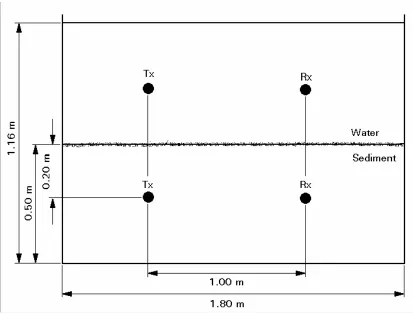
The speed of sound in sediments can be predicted using various models. It should be noted that several types of wave can propagate through sediments, i.e., compressional, shear and interface waves [21]. However, for the purpose of this investigation, only the normal compressional wave (or ‘p-wave’) is considered in any detail. (The existence and consequences of the other waves are considered in the next report in this series4.) The speed of sound in sediment is dependent on the bulk moduli of the fluid, the solid grains and the frame [22]. It is generally accepted that phase dispersion in both seawater and in sediments is negligible over any practical frequency range. The sound speeds in the water and the sediment were measured using a simple arrangement of two hydrophones8 separated by a distance of 1 m ± 1 cm, as shown in figure 5. In the first arrangement the hydrophones were independently suspended in the middle of the water column. Hydrophone, Tx, was used as a source and was excited using a single-cycle sine wave pulse, having a centre frequency of 75 kHz9. The transmitted acoustic pulse was received by the second hydrophone, Rx. In the second arrangement, the hydrophones were positioned 20 cm below the water-sediment interface. A similar acoustic pulse was generated by Tx and received by Rx. The time delay between the output and the returned pulse was measured in both cases.

8

Brüel & Kjær type 8103 hydrophones were used in the experiments described in this report and in the experiments described in the reports referenced in footnotes 4 and 6. Although being termed ‘hydrophones’, which are transducers that convert sound into electricity [23], piezoceramic transducers of this type can also be used as acoustic sources.

9

Figure 5 Side view of the source / receiver arrangement for the speed of sound

measurements in water and water-saturated sediment in the laboratory tank.

The sound speeds were calculated from the travel times of the acoustic pulses. They were found to be 1 478 m s-1 in water and 1 692 m s-1 in the sediment, with an error of

± 2 % in each case. (This error was based on the tolerance in the misalignment of the hydrophones.) The water temperature, T, was measured to be 16.5 °C ± 0.5 °C and the atmospheric pressure, Patm, was measured to be 1 006 mbar ± 0.5 mbar.

The speed of sound in distilled water can be found from the empirical formula [24]:

cf t t t

(

)

P

g g g g g

g

. . . .

= + − + + + + ⎛

⎝

⎜ ⎞

⎠ ⎟ 1402 7 488 488 135 15 9 2 8 2 4

100

2 3 2 (1)

The calculated result for distilled water agrees with the measured result for the tank water to within the estimated error10. From a comparison of the measured sound speed with that shown in figure 4, it can be seen that the speed of sound in the tank was similar to that found in the deep ocean.

The agreement shown between the measured and theoretical values in water suggests that the measured value for the speed of sound in the sediment should be reasonably accurate. Unfortunately, a comparison with the measured values available in the literature is difficult since real sediments display a wide range of sound speeds (from 1500 - 1900 m s-1) depending on their composition and geographical location [25]. However, the same literature also indicates that sound speed increases with mean grain size. It is interesting to note that the sound speed measured in the laboratory tank corresponds to grain diameters of less than 100 µm, which compares favourably with the particle size distribution measured in section 2.1.2.

(Attenuation in the sediment was also of particular interest. There are relatively few measurements available in the literature for sandy sediments over the range of frequencies used in this investigation. Therefore, the attenuation in the sediment in the laboratory tank was measured, as described in section 2.2.4.)

2.2.2 The Attenuation of Sound in Seawater

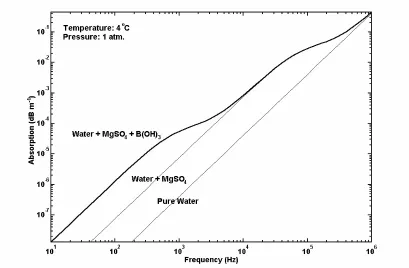
The attenuation of sound in seawater in the range 1 kHz - 1 MHz is attributed to three main absorption processes. The effects of shear viscosity [26] and volume viscosity [27] account for the absorption observed in distilled water, and in seawater the dominant cause of absorption at frequencies below 100 kHz is ionic relaxation. This is a chemical disassociation / reassociation process which occurs over a finite relaxation time [28].

Both the ionic relaxation mechanism and viscous absorption are dependent on frequency, salinity, temperature and pressure. An empirical equation based on laboratory data was presented by Fisher and Simmons [29, 31]. This result,

10

summarised in figure 6, includes the contributions from the two ionic compounds in seawater that have the strongest relaxation effect: magnesium sulphate and boric acid.

Figure 6 The absorption coefficient in seawater according to the expression of Fisher

and Simmons [29] in Lyman and Fleming seawater [30] of salinity 3.5 % and

pH = 8.0. The thick solid line is the combined absorption for pure water and the ionic

compounds, magnesium sulphate and boric acid.

2.2.3 The Attenuation of Sound in Suspensions

Small quantities of suspended material can have a significant effect on the attenuation of sound waves. In suspensions, attenuation is attributed to three main loss mechanisms: scattering by particles [3]; viscothermal absorption [32]; and the intrinsic absorption of acoustic energy by the water itself.

Scattering can be characterised in terms of the ‘form function’, which is proportional to the ratio of the re-radiated pressure to the incident pressure as a function of angle and distance from the scattering centre. When evaluated for monostatic scattering, it is proportional to the acoustic back-scatter cross-section [33, 34]. In general, theoretical models for the form function treat particles in suspension as a cloud of

homogeneous spheres [3] which exhibit characteristic resonances in response to an acoustic signal [35]. Conversely, naturally occurring sediments are irregular and inhomogeneous with the consequence that well-defined resonances do not occur.

Figure 7 The attenuation coefficient due to scattering and absorption as a function of

acoustic frequency and particle radius for a suspension of spherical quartz particles

with a mass concentration of 0.2 kg m-3 [36]. (Original in colour.)

Richards and co-workers [36] have taken a different approach to the scattering mechanism, using a heuristic model based on a modified form of the ‘high-pass model’ [37] as employed by Sheng and Hay [38]. This model also includes viscothermal losses, whereby sound energy is converted to heat by friction in the viscous fluid boundary around particles in suspension [32], and the absorption effects detailed in section 2.2.2.

Recent experimental work using suspensions of spherical11 quartz particles has shown good agreement with the theoretical predictions for the attenuation coefficient [41]. The size distribution of a suspension of sand particles in the laboratory tank has been measured, as detailed in section 2.1.1. The distribution exhibits a peak at a radius of around 3 - 4 µm, which is close to the theoretical viscothermal absorption peak shown in figure 7. Also, the accompanying size distribution for particles in the sediment bed shows that a sizeable fraction of the sediment is composed of particles that are not far removed from the scattering peak shown in figure 7. These observations imply that the attenuation coefficient associated with a suspension of sediment in the laboratory tank should be high.

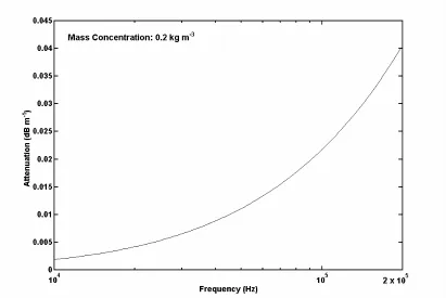
In order to estimate the attenuation coefficient for a real particle size distribution, the attenuation spectrum for each size bin must be calculated individually. The weighted sum of these spectra gives the total attenuation spectrum, where the weighting for each size bin is equal to the product of bin height and width. This calculation was performed for the measured distribution of sand grains in suspension with an arbitrarily chosen mass concentration of 0.2 kg m-3, as shown in figure 8.

The concentration of suspended material used in this calculation is unusually high for deep water regions, being more typical of the concentrations found in coastal and estuarine waters [36]. The total attenuation would be significant for high frequency sonar systems which operate in such regions over path lengths of up to several hundred metres [42]. However, for the purpose of this investigation, where the total path length and the concentration of suspended material are considerably less, the total attenuation was considered negligible.

11

Figure 8 The attenuation coefficient calculated for a suspension of sand particles in

the laboratory tank with a mass concentration of 0.2 kg m-3.

2.2.4 The Attenuation of Sound in the Seabed

It is generally accepted that sound energy is absorbed in the seabed by a combination of frictional losses at inter-particle contacts, and by viscous losses caused by the movement of the pore fluid relative to the solid frame [43]. However, the precise details of the attenuation mechanism are subject to debate. (It is noted in section 2.2.1 that several types of wave can propagate in sediments in addition to the primary compressional wave. These are considered in detail in the next report in this series4.) A considerable body of attenuation data is available in the literature for a range of sediment types at numerous geographical locations. On the basis of this evidence it has been argued by researchers such as Hamilton [2] that the attenuation coefficient,

αdB, of plane compressional waves in marine sediments varies with frequency, fk,

according to the relationship

α _α α

dB k

n

k f

= (5)

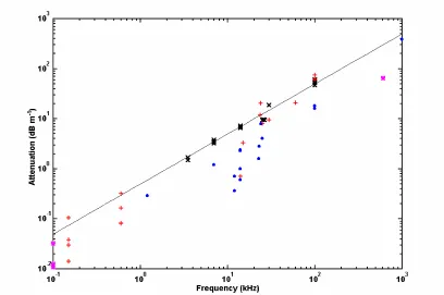
Attenuation appears to scale linearly with the first power of frequency (i.e., nα = 1) over the range of measurements shown in figure 9. It is useful to approximate the attenuation coefficient by using a value of kα = 0.5 (shown on the graph as a solid

line). This approximation is reasonably accurate for the available sand data and a good estimate for the data pertaining to sand, silt and clay. However, there are still relatively few measurements for sandy sediments between 10 kHz and 100 kHz (the frequency range that is of particular interest in this investigation).

The attenuation coefficient for the sediment in the laboratory tank was measured using a broadband pulse technique and a simple attenuation model. An ‘in-situ’ technique was preferred over the more conventional method of measuring attenuation with an impedance tube [44]. This was because it was desirable to minimise the disturbance to the sediment in the laboratory tank. Also, it was difficult to ensure that sediment taken from the tank did not contain any air or excess water, or that the size distribution did not change as a result of small particles being swept up into the water column.

The preferred method would have been to generate a single-frequency, continuous-wave (CW) acoustic signal from a source buried in the sediment, and to have measured the sound pressure at various distances from the centre of the source. Repeating the measurement for a range of different frequencies would have allowed the attenuation spectrum to have been determined with a high degree of accuracy. Unfortunately, CW signals could not be used effectively in the laboratory tank because of its relatively small size. Reflections from the tank walls, etc., would have interfered with the signal at the receiver within too short a time frame to have allowed useful measurements to be obtained.

Figure 9 The attenuation coefficient measured in a range of naturally occurring,

saturated marine sediments [2, 25, 45]. Symbols: × = sands, all grades; + = sand-silt,

silt-sand, sand-silt-clay; • = clay-silt, silt, silt-clay; and 6 = various clays. The

straight line corresponds to an attenuation coefficient of αdB =0 5fk

1

. . (Original in

colour.)

In practice, a 1 ms long chirp pulse, sweeping upwards in frequency from 20 kHz to 150 kHz, was used to drive the acoustic source. A 1/10 cosine-tapered window was applied to minimise transient distortion, resulting in the useful frequency range of the pulse being reduced to 33 - 137 kHz. The duration of the pulse was chosen to be as long as possible before reflections within the tank would have become a problem. The arrangement of the acoustic source, Tx, and receiver, Rx, are shown in figure 10. Hydrophones were used as both source and receiver elements. The first hydrophone, Tx, was positioned 25 cm below the water-sediment interface and near to one end of the tank. The second hydrophone, Rx, was positioned at a similar depth and near to the opposite end of the tank. For each set of measurements the position of Tx was

kept fixed and Rx was moved progressively closer. The distance between the two hydrophones, x, was noted in each case with an estimated accuracy of ± 1 cm.

Figure 10 Side view of the source / receiver arrangement for the sediment attenuation

measurement in the laboratory tank. The filled symbols represent the initial positions

of the acoustic source, Tx, and receiver, Rx. The outlined symbol represents the range

of positions of the receiver.

In order to interpret the signals recorded at the receiver, it was necessary to formulate a simple attenuation model. It was assumed that all measurements were performed in the far-field of the transducers and that they exhibited an omni-directional response12. Thus, a simple geometrical spreading function was used, with pressure amplitude varying as the inverse of distance. By assuming that the contribution due to noise was

12

negligible, a frequency-domain representation of the recorded signal, S(ω), can be written:

( )

( ) ( )

Sω = Ψ ω H ω (6)

where Ψ(ω) is the driving signal and H(ω) is the transfer function of the complete physical system. Both S(ω) and H(ω) are functions of frequency and of the separation between the source and receiver, x.

The transfer function can be separated into its separate components,

( )

[

( )

]

( )

H a x X

x

np

ω =exp − ω ω 1_∆ (7)

where X(ω) is the response of the detection system (including the signal generator, charge amplifier, power amplifier, etc.), anp is the attenuation coefficient in np m-1 (where α_dB =

(

)

(

)

ln = Ψ + − _np −∆ (8)

The directivity function, ∆, is equal to unity in the far-field. Given the separation, x, this equation can be expressed in terms of just two parameters:

(

)

By taking measurements at two positions, x1 and x2, and subtracting, the constant parameter disappears to leave

(

)

(

)

lnS_{x x=} −lnS_{x x=} = lnx −lnx −anp x −x

2 1 ∆ 1 2 1 2

(9)

which only has one unknown, anp.

form of equation (9). The average of n estimates of the attenuation coefficient gives a much more accurate value13.

In total five sets of data were recorded over two days, separated by a period of several weeks. The water temperature and the atmospheric pressure were recorded as being 15.5 °C ± 0.5 °C and 1014 mbar ± 0.5 mbar on the first day, and 16.2 °C ± 0.5 °C and 1016 mbar ±0.5 mbar on the second day. Each set of data comprised 21 measurements spaced 2.5 cm apart, with every measurement being the average of 100 recorded pulses. Thus, the five sets of data each provided 20 estimates of the attenuation coefficient; 100 estimates in total. The averaged results are presented in figure 11, alongside the historical data for attenuation measured in sands. The straight line on the graph corresponds to the approximation, α_dB =0 5. f_k1.

The attenuation measured in the laboratory tank was slightly less than that measured in the naturally occurring sands though it closely follows the empirical law, scaling linearly with the first power of frequency. A best-fit line, following the linear scaling law, was fitted to the laboratory data using a regression algorithm. The value of kα

was found to be 0.41 with a standard error on the regression estimate of 2.5 dB m-1. It should be noted that the acoustic insertion loss [48] experienced by hydrophones when they are used in sediment differs from that when they are used in water. In order to determine this difference, a similar set of measurements was obtained in water and a best-fit line was fitted to this new data. By comparing the standard errors on the regression estimates for the in-water and in-sediment measurements, an estimate of the insertion loss associated with hydrophone measurements in water-saturated sand was obtained. The sensitivity of the hydrophone in sand was found to vary by around

± 1 dB from its in-water sensitivity.

13

Figure 11 The average attenuation coefficient measured in the laboratory sand is

marked by the curve. The error bars at selected frequencies correspond to a standard

deviation of ± 1. A subset of the historical data (see figure 9) for a range of sandy

sediments are marked by the points, ×. The straight line corresponds to an attenuation

coefficient of α_dB=0 5. f_k1.

The attenuation of sound in the sediment is the most important attenuation process thus far considered, having a significantly greater effect than the attenuation processes in water and suspensions of particulate material. A comparison of the different sources of attenuation and the implications for an acoustic detection system are presented in section 2.3.

2.2.5 The Seawater-Seabed Interface

with particular consideration given to roughness scattering at the interface, is dealt with in the next report in this series4.

In the initial stages of the investigation it was assumed that the sediment could be modelled as a simple, homogeneous fluid with a plane interface. In this case, energy is divided between reflected and refracted compressional waves with the angle of transmission depending on the angle of incidence and the acoustic properties of the fluid media [50]. It has been noted by other authors that useful results can still be obtained with this approach [51].

Consider a scalar wave, ψi, incident on the boundary with reflected and transmitted waves ψr and ψt respectively. The required boundary conditions are that the tangential field (along the interface in the x-direction), ψx, is continuous and that ψi+ψr =ψt.

No assumptions are made about the directions of the reflected and transmitted waves. It can be shown that the angle of reflection is equal to the angle of incidence and that the angle of transmission of the refracted wave is governed by Snell’s law [52]:

sinθ_i sinθ_t c1 c2

= (10)

where θi and θt are, respectively, the angles of incidence and transmission of waves going from the first medium, with a sound speed, c1, into the second medium, with a sound speed, c2.

At a critical angle of incidence, θc, the angle of transmission reaches 90°. It is evident that for θi ≥θc no energy is transmitted into the second medium and the incident wave is said to undergo ‘total internal reflection’ [53]. However, if there is no transmitted wave the boundary condition (ψi+ψr =ψt) cannot be satisfied. Therefore, it is

asserted that a transmitted wave does exist but that it cannot, on average, carry energy across the boundary. This leads to a transmitted field vector of the form,

(

)

[

(

)

]

Ψt =Aexp mBz exp jωt−k xi sinθi (11)

penetrates the second medium. This disturbance travels along the interface in the x direction and is known as an ‘evanescent wave’ [53].

If the ‘fluid-fluid’ interface is assumed to be massless, the pressure amplitude transmission, TPa, and reflection, RPa, coefficients can be found from the conservation of particle velocity and the continuity of pressure at the boundary [52]:

R Z Z

Z Z Pa t i t i = − + 2 1 2 1 cos cos cos cos θ θ

θ θ and TPa = +1 RPa

(12)

where Z1 and Z2 are the characteristic acoustic impedances of the media (the product of volume density and the thermodynamic speed of sound). For sediments of low porosity, e.g., red clay, calcareous ooze, silt and fine quartz sand, the assumption of a simple reflection loss is often valid [54].

The power transmission, Tπ, and reflection, Rπ, coefficients are simply related to the pressure amplitude coefficients by R_π = R_Pa2 and T_π = −1 R_π. For the sediment in the laboratory tank, Rπ was calculated to be less than 0.3 for angles of incidence up to, approximately, 50°.

2.3 Summary of design considerations for sediment tank

In sections 2.1 and 2.2, above, the acoustic test facility and the physical nature of the acoustic media have been described. The sediment was principally composed of sand particles which were, to a first approximation, spherical and similar in size to sand particles found in the deep ocean. Their size distribution was measured using an optical technique and was found to be bimodal with peaks at effective spherical radii of a few microns and around 100 µm.

historical data for similar sediment types cover a wide range of sound speeds. Hence, no direct comparison could be made.)

Attenuation has been estimated for each component of the propagation path, i.e., the water, suspensions, and the sediment. The attenuation of sound in water is covered, extensively, in the literature. In seawater, the attenuation coefficient is, typically, around 10-2 dB m-1 in the 10 - 100 kHz range [29]. In pure water, it is an order of magnitude lower.

The attenuation of sound in suspensions is a relatively new topic of research. In the literature, theoretical models show good agreement with practical measurements for spherical particles, and limited agreement for non-spherical particles [41]. The attenuation associated with a suspension of sand in the laboratory tank was calculated using the particle size distribution data, noted above. Even for an artificially high concentration of suspended material (0.2 kg m-3), the attenuation coefficient was still found to be negligibly small (less than 5 × 10-2 dB m-1) in the 10 - 100 kHz range. The attenuation of normal compressional waves in the sediment has also been considered. A set of measurements were performed in the laboratory tank, and a value for the attenuation coefficient was calculated using a simple attenuation model. It was found to scale linearly with frequency, although the value obtained for the laboratory sand was slightly lower than in naturally occurring sands (by 0.09 dB m-1 kHz-1). It should also be noted that sands are, generally, more highly attenuating than other sediment types such as silts and clays.

range, the attenuation coefficient in water-saturated sand varies from 5 - 50 dB m-1 (compared with attenuations of less than 0.1 dB m-1 in water and suspensions).

The implication for a detection system is quite obvious. The sound pressure developed by the source must be high enough that acoustic waves can penetrate the sediment, and usefully interact with a target buried at a depth of up to 1 m. However, an increase in the acoustic power of the source is necessarily accompanied by an increase in the reverberation level in the medium, i.e., the scattering of the emitted signal from the seabed surface and volume inhomogeneities within the sediment [33]. Hence, the receiver must be designed to have a narrow beamwidth, in order to prevent reverberant energy from dominating the incoming acoustic signal. The design of the transducer system is presented in section 3. In addition, signal processing techniques can be used to extract useful target information from high levels of background noise and clutter. Several approaches, ranging from simple time windowing to more advanced techniques, such as optimal filtering, are presented in a later report in this series6.

3 Transducer

Design

A source and receiver can be arranged either monostatically or bistatically, i.e., the source and receiver can be combined in a single unit or they can be located separately. Ordinarily, a monostatic arrangement would be the preferred choice for an ROV-mounted system. (ROVs are generally built to house modular, compact devices, and a single unit would offer advantages in terms of ruggedness, ease of alignment, simplicity of installation, etc.) However, in the laboratory it was considered better to use separate units that would be easier to install and operate.

Many commercial sonar systems exhibit such characteristics [55]. Notable amongst these are parametric sonar systems [56] that exploit the non-linear property of water,

i.e., a change in density caused by a change in pressure of a sound wave in water is not linearly proportional to the change in pressure. In any such non-linear system, the frequencies produced at the output are different to those at the input. These secondary frequencies, which may include harmonic and sub-harmonic frequencies, only occur at ‘high’ amplitudes of the primary wave. With a parametric sonar there is no sidelobe radiation outside of the main beam; the beamwidth is narrow and nearly constant over a broad range of frequencies; the sonar exhibits an inherently broad bandwidth; and projector cavitation does not pose a problem. However, systems such as these were considered to be too expensive to be used in this study. Therefore, a directional transducer system was purpose-built for use in the laboratory. Fortunately, there was considerable scope in the design of the transducers to enable a high power and narrow beamwidth to be achieved. Two techniques were considered in some detail:

• Beamforming. The interference pattern that results from the linear superposition of an array of monopole sources radiating at the same frequency can have a pronounced directivity [57]. This can be controlled by changing the relative phase of the sources. For the purpose of this investigation, an ‘ideal’ beam pattern would comprise a narrow central lobe with minimal sidelobes. However, in a highly directional array a significant proportion of the source power can leak away to the sidelobes. This can be reduced by applying a windowing function to the array, but only at the expense of directionality.

It should be noted that classic array signal processing techniques assume that plane waves are reformed at the array, i.e., operations are performed in the acoustic far-field. Array techniques become sub-optimal close to the array. Furthermore, the range of frequencies that can be generated before spatial-aliasing occurs is limited by the separation of the sources [58].

relative to the back of the reflector. However, the relationship between the source position and the focus is logarithmic which can make it difficult to set the focal length accurately.

The acoustic reflector and the beamforming array are both established techniques for producing a tightly confined acoustic beam. The array has the advantage of being able to produce a higher output power than the reflector because more than one source element is involved. However, on the grounds of its relative simplicity and cost-effectiveness, the acoustic reflector approach was adopted for this application.

Some alternative techniques have also been considered. For example, iterative, time-reversal focusing could provide a means of developing a high acoustic power in the region of the target [60, 61, 62]: An array of transmit and receive transducers can be used to insonify a target volume and record the back-scattered signals. If these signals are time-reversed and re-emitted, the transmitted signal should refocus on any reflective scatterer within the target volume. If the medium is largely homogeneous, but contains several scatterers, the time reversal process can be made to focus on the most reflective one by iteration. The array can also be curved, like the acoustic reflector, to become both electronically and geometrically focused [63].

This approach would seem to combine the best of both transducer designs (i.e., high power, narrow beamwidth, and electronically adjustable focusing) and would be a natural extension of the acoustic reflector arrangement for use in the field. However, there are two major drawbacks associated with this method: it becomes ineffective if the attenuation in the surrounding medium is high; and substantial computing power is required.

3.1 The Design of an Acoustic Reflector

to a parabola in the paraxial focusing region and, in general, will suffer less aberration than its aspheric counterparts. Spherical mirrors are also much easier to fabricate than aspheric surfaces, especially in the case of large reflectors. This is an important consideration since surface features must be controlled to within much less than the wavelength of the incident radiation to keep diffraction to a minimum.

In order to collect as much of the source power as possible, a large reflector aperture was required. Buckingham used a 3 m diameter, spherical reflector in his acoustic daylight™ experiments [59, 65]. This comprised a pressure-release surface made from neoprene rubber bonded to a fibreglass shell. Potter later demonstrated that a smaller dish would have resulted in a better confinement of the acoustic beam [66]. In this investigation, the maximum reflector size was constrained by the dimensions of the laboratory tank and, to some extent, by the cost of fabrication. Therefore, a simple comparison between a range of reflectors having different diameters was performed using a ray tracing algorithm.

A description of the reflector geometry and the details of the algorithm used to determine its focusing characteristics are presented in appendix A. The caustic curve bounding the acoustic field was found by the application of Fermat’s principle [67]. This states that the actual ray path between two points is the one that is traversed in the least time. A useful figure of merit for the caustic is the diameter of the circle of least confusion, ΣLC [68]. The acoustic intensity should be high in this region since this is the part of the caustic that has the smallest diameter.

The acoustic source positions were selected such that the paraxial foci were produced at an arbitrarily chosen distance of 2 m from the back of each reflector using the lens-maker’s formula (see appendix A, equation (A 7)). The longitudinal and transverse spherical aberrations (LSA and TSA respectively) for three different aperture radii are presented in table 1. Also shown is the angle θr measured at the sound source and subtended between the rim of a spherical reflector and the acoustic axis.

rr (m) ΣLC (m) LSA (m) TSA (m) θr (rad)

0.125 0.055 1.498 0.399 1.177 0.150 0.061 1.412 0.383 1.170 0.175 0.067 1.330 0.366 1.163 Table 1 Simulation results for 25, 30 and 35 cm diameter spherical reflectors.

It was expected that the larger the aperture, the larger the spherical aberration that would be observed. This is true if the position of the source is fixed relative to the back of the reflector. However, in this analysis (and in practice) it was the position of the focus that was fixed. It can be seen that both the longitudinal and the transverse spherical aberrations actually improve with the larger dish. The penalty, however, is that the source must be moved slightly farther from the reflector such that the angle,

θr, reduces and the diameter of the circle of least confusion, ΣLC, increases. Thus, the

Spherical aberration was considered to be a more important factor than confinement within the circle of least confusion. (The reason for this is better illustrated in a practical measurement, as shown in the next section.) Therefore, the larger, 35 cm diameter reflector size was chosen. Two such reflectors were cut from a block of closed-cell expanded polyurethane foam, according to the design specification shown in figure 12. To limit scatter, the surface tolerance was specified to be ± 1 mm, i.e., around 1/20 of an acoustic wavelength at 75 kHz in water.

The reflector material was chosen on the basis that the polyurethane frame would be robust enough to withstand handling whilst the air trapped within the closed pores would ensure a large acoustic impedance mismatch in water. Alternative reflector materials were also considered, but polyurethane foam was decided to be the best to use on the grounds of cost and the ease of fabrication.

Hydrophones were used as both the acoustic source and receiver elements. As noted in footnote 12, manufacturer’s data indicates that the variation in their sensitivity should have been less than 3 dB in every direction at a frequency of 100 kHz or less [47]. In order to confine their directional responses to within the collection angles of the reflectors, back-reflectors were attached to each of the hydrophones.

3.2 Free-Field Characterisation

The performance of one of the reflectors was assessed when acting as an acoustic source. It was submerged in a large (8 m × 8 m × 5 m deep) water tank14, which allowed side-wall reflections to be removed by time windowing. It proved very difficult to adjust the paraxial focus accurately because of the non-linear relationship between the focus and source positions. Therefore, the hydrophone was carefully positioned and fixed at a distance of S0 = 13 cm from the back of the reflector such that the paraxial focus was, in theory, close to infinity. (This setup was maintained throughout all the subsequent experiments that involved the reflectors by the use of thin steel rods which held the hydrophones firmly in place.)

14

The hydrophone, when used as an acoustic projector, was driven by a series of single-cycle sine wave pulses, each having a centre frequency of 75 kHz (cf., section 2.2.1 and footnote 9). The acoustic pressure amplitude that resulted from each pulse was recorded at discrete points in front of the reflector using an independent hydrophone.

Sound Pressure Level (dB re 1 µPa)

Figure 13 The sound field generated by a focused acoustic reflector (focusing at ∞). The crosses represent discrete measurement positions and the solid line delineates the

theoretical boundary of the acoustic field. (Original in colour.)

The measured sound field is shown in figure 13. The value at each of the sample points, ×, is the intensity level, IL; the pulse-averaged intensity measured at the receiver, Ipa, divided by a reference intensity, Iref, and expressed using a logarithmic scale, IL=10log₁₀

(

)

(

)

Pe is an effective pressure and Pref is a reference pressure [69, 70]. A continuous image was obtained using piecewise, bilinear interpolation between the sampling points. The solid outline delineates the theoretical boundary of the acoustic field, i.e., the back of the reflector and the caustic.

It can be seen that the highest energy density coincides with the point at which marginal rays cross the acoustic axis, i.e., the position of the LSA. (It should be noted that the ray tracing model is, at best, an approximation for marginal rays, since diffraction effects are most severe at the rim of the reflector.) The LSA associated with the smaller reflectors (see table 1) would have caused the high energy region to be closer to the acoustic projector. Therefore the choice of the larger, 35 cm diameter reflector proved to be the most appropriate for producing a high energy density at the greatest range in the medium.

A quantity known as the directivity index is often used to measure the performance of an acoustic source [57]. It is defined as the ratio of the intensity of a directional source at some distance on the acoustic axis to the intensity of a simple (omni-directional) source at the same distance. The directivity index of the focused acoustic reflector was estimated to be greater than 20 dB from the data shown in figure 13 and from a measurement of the intensity of an unfocused source at the same distance as the circle of least confusion of the focused source.

3.3 Transmission Loss

The transmission loss associated with a focused acoustic beam propagating in the sediment was investigated using a reflector / hydrophone used as an acoustic source, Tx, and an independent hydrophone acting as a receiver, Rx. The water-sediment interface was given to be flat such that sound would be transmitted into the sediment in the same way, regardless of where it was projected on the interface.

Figure 14 The source / receiver arrangement for the sediment transmission loss

measurement in the laboratory tank. The filled symbols represent the initial positions

of the acoustic source, Tx, and receiver, Rx. The outlined symbols represent the range

of positions of Tx and Rx.

Hence, it was possible to obtain a two-dimensional measurement by moving the receiver vertically (i.e., in the z-direction) within the sediment and the reflector horizontally (i.e., in the x-direction) above it. This approach caused less disturbance to the sediment than would have been the case if the source was kept at a fixed position and the receiver was moved horizontally as well as vertically. The source / receiver arrangement is shown in figure 14.