GDP Festschrift ENTCS, to appear
A Bayesian model for event-based trust
Mogens Nielsen
1Karl Krukow
2BRICS
University of Aarhus, Denmark3
Vladimiro Sassone
ECS, University of Southampton
Abstract
The application scenarios envisioned for ‘global ubiquitous computing’ have unique re-quirements that are often incompatible with traditional security paradigms. One alternative currently being investigated is to support security decision-making by explicit representa-tion of principals’ trusting relarepresenta-tionships, i.e., via systems for computarepresenta-tional trust. We focus here on systems where trust in a computational entity is interpreted as the expectation of certain future behaviour based on behavioural patterns of the past, and concern ourselves with the foundations of such probabilistic systems. In particular, we aim at establishing formal probabilistic models for computational trust and their fundamental properties. In the paper we define a mathematical measure for quantitatively comparing the effectiveness of probabilistic computational trust systems in various environments. Using it, we com-pare some of the systems from the computational trust literature; the comparison is derived formally, rather than obtained via experimental simulation as traditionally done. With this foundation in place, we formalise a general notion of information about past behaviour, based on event structures. This yields a flexible trust model where the probability of com-plex protocol outcomes can be assessed.
1
Introduction
Part of the Grand Challenge of a science for global ubiquitous computing (GUC) [5] is to find alternatives to existing approaches to access control, and, more
gener-1 Email:[email protected] 2 Email:[email protected]
3 BRICS: Basic Research in Computer Science (www.brics.dk),
ally, security sensitive decision making. Many features of GUC (virtual anonymity, scalability, mobility, autonomy, ubiquity, incomplete information, global connec-tivity, . . . ) will affect our notion of security requirements. For example, mobility implies that a GUC entity might find itself in a hostile environment, disconnected from its preferred security infrastructure, e.g., its usual certification authorities. Further, the autonomy requirement means that even in this scenario, it must be able to assign privileges to other GUC entities; privileges that are meaningful based on usually incomplete information the assigning entity has about the assigned entity. These properties of GUC imply that traditional security mechanisms are no longer applicable (see e.g., Blaze, Feigenbaum et al [1]). One of the alternatives currently being investigated is an approach based on the notion of trust that, in some ways, re-sembles the concept of trust as it exists among human beings. We refer to this line of research as computational trust. In fact, computational trust deals not merely with access control, but more generally with decision making by computational agents in the presence of unknown, uncontrollable and possibly harmful entities. This is the case for e.g. the autonomous selection of (apparently similar) providers of particular services.
In the area of computational trust it is hard to identify one model (or even a few) accepted widely by the community. The GUC feature of incomplete information naturally leads to probabilistic decision making; hence, one common classification distinguishes between ‘probabilistic’ and ‘non-probabilistic’ models [8,21,13]. The non-probabilistic systems may be further classified into different types (e.g., so-cial networks or cognitive); in contrast, the probabilistic systems usually have a common objective and structure: they (i) assume a particular (probabilistic) model for principal behaviour; and (ii) put forward algorithms for approximating the be-haviour of principals (i.e., for making predictions in the model). In such models the trust information about a principal is information about its past behaviour, its history. Such histories do not immediately classify principals as ‘trustworthy’ or ‘untrustworthy,’ as ‘good’ or ‘bad;’ rather, they are used to estimate the probabil-ity of potential outcomes arising in a next interaction with an entprobabil-ity. Probabilistic systems, called ‘game-theoretical’ by Sabater and Sierra [21], are based on Gam-betta’s view of trust [9]:“. . . trust (or, symmetrically, distrust) is a particular level of the subjective probability with which an agent assesses that another agent or group of agents will perform a particular action, both beforehe can monitor such action (or independently of his capacity ever to be able to monitor it) andin a context in which it affectshisown action.”
the event structure framework we previously used in the SECURE project [4], and we use it to model outcomes of interactions and make predictions using Bayesian learning on their configurations. In this sense, our framework generalises previous probabilistic models with only ‘binary’ outcomes [16,8,22] – i.e., where each in-teraction is perceived as either ‘good’ or ‘bad’ – to multiple, structured outcomes. Such outcomes may in simple cases represent different degrees of satisfaction on the ‘good’–‘bad’ scale, or in more complex cases exploit the full expressive power of event structures’ causation mechanisms.
Bayesian analysis consists of formulating hypotheses on some real-world phe-nomenon, running experiments to test such hypothesis, and thereafter updating the hypotheses –if necessary– to provide a better explanation of the experimental obser-vations, a better fit of the hypotheses to the observed behaviours. By formulating it in terms of conditional probabilities on the space of interest, this procedure is expressed succinctly in formulae by Bayes’ Theorem:
Prob(Θ|X) ∝Prob(X|Θ)·Prob(Θ).
Reading from left to right, the formula is interpreted as saying: the probability of the hypothesesΘposterior to the outcome of experiment X is proportional to the likelihood of such outcome under the hypotheses multiplied by the probability of the hypotheses prior to the experiment.4 In the present context, the priorΘ will be an estimate of the probability of each potential outcome in our next interaction with principal p, whilst the posterior will be our amended estimate after one such interaction took place with outcome X.
It is important to observe here that Prob(Θ | X) is in a sense a second order notion, and we are not interested in computing it for any particular value of Θ. Indeed, as Θ is the unknown in our problem, we are interested in deriving the entire distribution in order to compute its expected value, and use it as our next estimate forΘ.
In order to make this discussion more concrete, let us first focus on a model of binary outcomes. Here Θ can be represented by a single probability Θp, the
probability that principal p will behave benevolently, i.e., that an interaction with p will be successful. In this case, a sequence of n experiments X = X1· · ·Xn is a
sequence of binomial (Bernoulli) trials, and is modelled by a binomial distribution Prob(X consists of k successes)= Θkp(1−Θp)n−k.
It turns out that if the priorΘfollows aβ-distribution, say B(α, β)∝ Θα−1
p (1−Θp)β−1
of parametersαandβ, then so does the posterior: viz., if X is an n-sequence of k successes, Prob(Θ | X) is B(α+ k, β+ n − k), the β-distribution of parameters
α+k and β+n−k. This is a particularly happy circumstance when it comes to
4 We shall often omit the proportionality factor, as that is uniquely determined as the constant that
apply Bayes’ Theorem, because it makes it straightforward to compute the posterior distribution and its expected value from the prior and the observations; it is known in the literature as the condition that theβ-distribution family is a conjugate prior for the binomial trials.
As described above, our model of choice departs from the view of interaction as a sequence of events with binary (success/failure) outcomes. Technically, we see configurations of finite, confusion-free event structures as arising from sequences of independent, multiple probabilistic choices. Mathematically, this entails passing from the binomial distributions typical of binomial trials to multinomial distribu-tionsΘn1
1 . . .Θ
nk
k (with
PΘ
i = 1) typical of n-sequences of trials (n = Pni) with k
distinct outcomes. In this new framework, our Bayesian analysis relies on observ-ing sequences of event structure configurations –one event at the time– to ‘learn’ (i.e., estimate) the probability of each configuration occurring as the outcome of the next complex (sequence of elementary) interactions. Here of courseΘi represents
our current estimation of the probability that the ith event in the k-way choice. Cor-respondingly, we need to identify a suitable conjugate prior to multinomial trials, to replace theβ distribution in the application of Bayes’ Theorem. As we explain in§4, we identify it in the family of Dirichlet distribution
D(α1, . . . , αk)∝Θα11−1· · ·Θ
αk−1
k .
In complete analogy with the binary case, and thus determining a smooth and uni-form lifting of the theory, if the prior follows a Dirichlet distribution D(α1, . . . , αk),
then the posterior Prob(Θ| X) follows the Dirichlet distribution D(α1+#1(X), . . . , αk +#k(X)),
where #i(X) counts the occurrences of event i in the sequence X. We remark that a
similar observation was independently made in [11,20].
Structure of the paper. The paper is organised as follows. In§2 we make precise the scenario illustrated somehow informally in the Introduction, and prove our re-sults on the formal of computational trust algorithms. For simplicity, we present our arguments in the case where experiments are sequences of unstructured outcomes; indeed, we expect all of them to go through mutatis mutandis to the case where outcomes are event structure configurations. The rest of the paper is dedicated to lifting the binary model to structured, distributed, complex outcomes afforded by event structures. In §3 we introduce the model of probabilistic event structures; readers acquainted with [23] may safely omit this section. In §4 we equip event structures with Dirichlet distributions, and illustrate our event-based framework for Bayesian analysis. Finally,§5 reflects on some of the basic hypotheses of the prob-abilistic models illustrated in the paper, and points forward to future research aimed at relaxing them.
2
Bayesian models for trust
At the outset, Bayesian trust models are based on the assumption that principals behave in a way that can profitably be approximated by fixed probabilities. Ac-cordingly, while interacting with principal p one will constantly experience out-comes as following an immutable probability distribution Θp. Such assumption
may of course be unrealistic in several real-world scenarios, and we shall discuss in§5 a research programme aimed to lift it; for the moment however, we proceed to explore where such an assumption leads us.
Our overall goal is to obtain an estimate ofΘpin order to inform our future
pol-icy of interaction with p. Computational trust algorithms attempt to do this using Bayesian analysis on the history of past interactions with p. Let us fix a proba-bilistic model of principal behaviour, that is a set of basic assumptions on the way principals behave, sayλ, and then consider the behaviour of a single, fixed principal p. We shall focus on algorithms for the following problem: let X be an interaction history x1,x2, . . . ,xn obtained by interacting n times with p and observing in
se-quence outcomes xi out of a set{y1, . . . ,yk}of possible outcomes. A probabilistic
computational trust algorithm, sayA, outputs on input X a probability distribution on the outcomes{y1, . . . ,yk}. That is,Asatisfies:
A(yi | X)∈[0,1] (i=1,...,k)
k
X
i=1
A(yi | X)=1.
Such distribution is meant to to approximate aΘpunder the hypothesesλ. To make
probabilities:
Prob(yi |Xλ) : the probability of “observing yi in the next interaction,
given the past history X;”
Prob(X|λ) : the a priori probability of “observing X in the modelλ.” Now, Prob(· | Xλ) defines the ‘true’ distribution on outcomes for the next interac-tion (according to the model); in contrast, A(· | X) aims at approximating it. We shall now propose a generic measure to ‘score’ specific algorithmsAagainst given probability distributions. The score, based on the so-called Kullback-Leibler diver-gence, is a measure of how well the algorithm approximates the ‘true’ probabilistic behaviour of principals.
2.1 Towards Comparing Probabilistic Trust-based Systems
Closely related to Shannon’s notion of entropy, Kullback and Leibler’s information divergence [15] is a measure of the distance between two probability distributions. For p = (p1, . . . ,pk) and q = (q1,q2, . . . ,qm) distributions on a finite set of events,
the Kullback-Leibler divergence from p to q is defined by
DKL(p kq)= k
X
i=1
pilog2(pi/qi),
where the log-base used is immaterial. Information divergence resembles a distance in the mathematical sense: it can be proved that DKL satisfies DKL(p k q) ≥ 0 and that equality is obtained if and only if p =q; however, it fails to be symmetric. We adapt DKL to score the distance between algorithms by taking the its average over possible input sequences, as illustrated below.
For each n∈N, let Ondenote the set of interaction histories of length n. Define
Dn
KL, the nth expected Kullback-Leibler divergence fromλtoAas: DnKL(λ k A)= X
X∈On
Prob(X|λ)·DKL Prob(· | Xλ)k A(· | X),
That is,
DnKL(λ k A)= X X∈On
Prob(X|λ)·
k
X
i=1
Prob(yi | Xλ) log2
P(yi | Xλ)
A(yi | X)
! .
the intrinsic probability of sequence X. In other terms, we compute the expected information divergence for inputs of size n.
While Kullback and Leibler’s information divergence is a well-established mea-sure in statistics, to our knowledge measuring probabilistic algorithms via Dn
KL is new. Due to the relation to Shannon’s information theory, one can interpret DnKL(λk A) quantitatively as the expected number of bits of information one would gain by knowing the ‘true’ distribution Prob(· | Xλ) on all training sequences of length n, rather than its approximationA(· | X).
2.1.1 An example.
In order to exemplify our measure, we compare the β-based algorithm of Mui et al [16] with the maximum-likelihood algorithm of Aberer and Despotovic [7]. The comparison is possible as the algorithms share the same fundamental assumptions that:
each principal’s behaviour is so that there is a fixed parameter Θ that at each interaction we have, independently of anything we know about other interactions, probabilityΘof ‘success’ and, therefore, probability 1−Θof ‘failure.’
We refer to these as the β-modelλB. With s and f standing respectively for ‘suc-cess’ and ‘failure,’ an n-fold experiment is a sequence X ∈ {s, f}n, for some n > 0.
The likelihood of X∈ {s, f}n is given by
Prob(X |ΘλB)= Θ#s(X)(1−Θ)#f(X),
where #x(X) denotes the number of occurrences x in X. UsingAandBto denote
respectively the algorithm of Mui et al, and of Aberer and Despotovic, we have that:
A(s|X) = #s(X)+1
n+2 and A( f |X)=
#f(X)+1 n+2 , B(s|X) = #s(X)
n and B( f |X)=
#f(X) n .
For each choice of Θ ∈ [0,1] and each choice of training-sequence length n, we can compare the two algorithms by computing and comparing Dn
KL(ΘλB k A) and Dn
KL(ΘλB k B).
Theorem 2.1 If Θ = 0 or Θ = 1, Aberer and Despotovic’s algorithmB from [7] computes a better approximation of the principal’s behaviour than Mui et al’s al-gorithmAfrom [16]. In fact, under the assumptions,Balways computes the exact probability of success on any possible training sequence.
while A(s | fn) = 1/(n+2)). Since Prob(s | fnΘλB) = Θ = 0 = B(s | fn) and Prob( f | fnΘλ
B)= 1−Θ =1= B( f | fn), we can conclude that DnKL(ΘλB k B)=0.
Since Dn
KL(ΘλBk A)>0 we are done. (The argument forΘ =1 is similar). Let us now compareAandBfor 0<Θ< 1. Observe thatBassigns probability 0 to s on input fk for all k ≥ 1; this results in Dn
KL(ΘλB k B) = ∞. It follows necessarily that in this caseAprovides a better approximation.
In order to explore the space of β-based algorithms further, we define a para-metric algorithmA, for ≥0, that encompasses bothAandB:
A(s|h)= #s(h)+
|h|+2 and A(s| X)=
#f(h)+
|h|+2 . Observe thatA0 =BandA1= A.
Let us now study the expression Dn
KL(ΘλB k A) as a function of . We shall prove that for eachΘ,1/2 and independently of n there is a unique which min-imises the distance Dn
KL(ΘλB k A). Furthermore, D
n
KL(ΘλB k A) is decreasing on the interval (0,¯] and increasing on the interval [¯,∞). (Notice of course that DnKL(ΘλB k A)→ ∞when →0.) By definition, we have:
DnKL(ΘλBk A)= n
X
i=0
n i
!
Θi
(1−Θ)n−i
"
ΘlogΘ(n+2)
i+ +(1−Θ) log
(1−Θ)(n+2) n−i+
# .
Isolating the terms that contain, we obtain
n X i=0 n i !
Θi(1−Θ)n−ih
ΘlogΘ +(1−Θ) log(1−Θ)i+log(n+2)
−
n
X
i=0
n i
!
Θi(1−Θ)n−ih
Θlog(i+)+(1−Θ) log(n−i+)i.
By differentiating DnKL(ΘλBk A) with respect to epsilon, we obtain d
dD n
KL(ΘλBk A)= 2α n+2 −
n X i=0 n i !
Θi(1−Θ)n−i
"
Θα
i+ +
(1−Θ)α n−i+
# ,
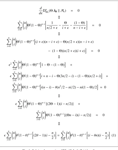
where α = log e is a positive constant obtained when differentiating the function log. In order to find a minimal point for the information diverge, let us examine which nullify the derivative d Dn
KL(ΘλB k A)/d. The bulk of the calculation is illustrated in Fig. 1. Observe that sincePn
i=0i
n
i
Θi(1−Θ)n−iis the expected number
d dD
n
KL(ΘλB k A) = 0 m
n
X
i=0
n i
!
Θi
(1−Θ)n−i
"
1 n/2+ −
Θ i+ −
(1−Θ) n−i+
# = 0 m n X i=0 n i !
Θi(1−Θ)n−ih
(i+)(n−i+)−Θ(n/2+)(n−i+) − (1−Θ)(n/2+)(i+)i = 0
m
2
n
X
i=0
n i
!
Θi(1−Θ)n−ih
1−Θ−(1−Θ)i +
n
X
i=0
n i
!
Θi
(1−Θ)n−ihi+n−i−Θ(3n/2−i)−(1−Θ)(n/2+i)i + n
X
i=0
n i
!
Θi(1−Θ)n−ih
i(n−i)−θ(n2/2−ni/2)−ni(1−Θ)/2i = 0 m
n
X
i=0
n i
!
Θi(1−Θ)n−i[(2Θ−1)(i−n/2)] + n X i=0 n i !
Θi(1−Θ)n−i[(Θn−i)(i−n/2)] = 0
m n X i=0 n i !
θi(1−θ)n−i(2θ−1)(i− n
2) = n X i=0 n i !
θi(1−θ)n−i(i−θn)(i− n
2)
[image:9.595.110.499.70.564.2]
(1)
Fig. 1. Solving the equation d DnKL(ΘλB k A)/d =0.
that
n
X
i=0
i2 n i
!
Θi(1−Θ)n−i =n(n−1)Θ2+ Θn.
These equalities lets us write equation (1) in a simpler form:
We therefore have(2Θ−1)(nΘ−n/2)=(2Θ−1)n(Θ−1)=(2Θ−1)2n/2,and n(n−1)Θ2+ Θn−Θn(n/2+ Θn)+ Θn2/2 =
n2(Θ2−Θ/2−Θ2+ Θ/2)+n(Θ−Θ2) = nΘ(1−Θ).
Since (2Θ−1)2is non-zero whenΘ,1/2, we obtain that d DKLn (ΘλB k A)/d is nullified if and only ifΘ, 1/2 and
= 2Θ(1−Θ) (2Θ−1)2 .
Remarkably, this is independent of n. Also, from the same derivation we immedi-ately obtain that
d dD
n
KL(ΘλB k A)<0 ⇐⇒ <
2Θ(1−Θ) (2Θ−1)2 and
d dD
n
KL(ΘλB k A)>0 ⇐⇒ >
2Θ(1−Θ) (2Θ−1)2 We have therefore proved the following.
Theorem 2.2 For anyΘ∈[0,1/2)∪(1/2,1] there exists ∈[0,∞) that minimises DnKL(ΘλB k A) simultaneously for all n; viz., =2Θ(1−Θ)/(2Θ−1)2.
Furthermore, Dn
KL(ΘλB k A) is a decreasing function of in the interval (0, ) and increasing in (,∞).
This means that unless the principal’s behaviour is completely unbiased, then there exists a unique best A algorithm that outperforms all the others, for all n.
If instead Θ = 1/2, then the larger the , the better the algorithm. Regarding A and B, an application of Theorem 2.2 tells us that the former is optimal for Θ = 1/2±1/√12, whilst –as anticipated by Theorem 2.1– the latter is such for Θ = 0 andΘ = 1.
Concluding this section, it is useful to remark that it is not so much the com-parison of algorithms AandB that interests us; rather, the message is that using formal probabilistic models enables such mathematical comparisons and, more in general, to investigate properties of models and algorithms.
3
Probabilistic Event Structures
the interaction begins. By behavioural observations, we mean observations that the parties can make about specific runs of such protocols. These include infor-mation about the contents of messages, diversion from protocols, failure to receive a message within a certain time-frame, and more. Here as in previous work (cf. [17,14,13]) we use event structures to formalise the concepts of protocols, obser-vations, and outcomes.
Event structures are well suited to our present purposes, as they provide a generic model for events (i.e., basic observables) and causation that is indepen-dent of any specific programming language and higher-level model. In our model, the information that an agent holds about another agent’s behaviour, is information about a number of protocol-runs with it, organised as a sequence of sets of events, or configurations, x1x2· · ·xn. Configuration xirepresents the ith run of the protocol
(e.g., ordered chronologically by starting times), and collects all the events hap-pened up to that point in that instance of the protocol; ximay represent a completed
protocol-run, in which case it records the complete outcome of an interaction, or an running one, in which case more events will be added to it as the computation proceeds. Note that, as opposed to many existing systems, here we are not rating the behaviour of principals; we are instead recording their actual behaviour, i.e., the precise events occurred in the interaction. We will later equip the model with probability measures so as to rate interaction outcomes and therefore assess the likelihood of future interactions.
Although event structures were the model of choice for computing ‘trust val-ues’ of distributed interactions in the SECURE project [3,4], we did not use in that context a formal probabilistic model of principal behaviour. In the next two sec-tions, we amend that: we augment event structure framework with a probabilistic model which generalises the one used in systems based on the beta-distribution [12,16,2,22], and we show how to compute the probabilities of outcomes given a history of observations. While this could be valuable in its own right, we remark that our primary reason is to illustrate an example of a formal probabilistic model which enables formal questions to be asked (and answered). The proposed system is not yet practical: there are in fact many issues it does not handle, as e.g., changes of principal behaviours, lying reputation sources, and multiple execution contexts. We believe that the basic probabilistic model must be better understood before we can deal with such issues successfully.
3.1 Event structures
They satisfy the following properties for all e,e0,e00 ∈E. [e]def= {e0 ∈E |e0 ≤e}is finite;
if e # e0 and e0 ≤e00 then e # e00
The intention behind all this should be intuitive. An event may exclude the pos-sibility of the occurrence of other events; this is what the conflict relation models. The necessity relation represents the idea that events are only possible when others, their causes, have already occurred. Finally, if two events are in neither of the rela-tions, they are said to be independent. The two conditions above are therefore that events must be finitely-caused and that conflict extents along with causation.
An event structure models the set of events that can occur in a particular pro-tocol; the control flow is provided by ≤ and #, that guarantee that not all sets of events can occur in a particular run. The notion of configurations formalises this as follows. A set of events x⊆ E is a configuration of ES if it is
Conflict free: for any e,e0 ∈ x : not e # e0; and
Causally closed: for any e ∈x,e0 ∈E : e0 ≤ e implies e0 ∈ x.
We writeCES for the set of configurations of ES. The set of all maximal config-urations, i.e., configuration that cannot be extended, defines the set outcomes of an interaction exhaustively. Such configurations are of course mutually exclusive.
3.2 Histories
A finite configuration models information regarding a single interaction, i.e., a sin-gle run of a protocol. In general, the information that one principal possesses about another consists of information about several protocol runs; the information about each individual run being represented by a configuration in the corresponding event structure. The concept of a (local) interaction history models this. An interaction history in ES is a finite ordered sequence of configurations, h = x1x2· · ·xn ∈ C∗ES.
The entries xiare called sessions of h.
3.3 Confusion-Free Event Structures
In the following we consider a special type of event structures, so-called confusion free, to which it is especially simple to adjoin probabilities [23]. As we shall see, the key for that is to assure that all ‘choice points’ –here called cells– are independent of each other. This amounts to requiring that the occurrence of an event does not affect the relative probabilities inside cells, even though it may of course rule out entire cells. This will be achieved by guaranteeing that each event belongs to at most one cell and that conflict behaves uniformly on cells.
Consider the following event structure as an aid to fix ideas in the following definitions (∼represents conflict, and→represents causality).
c /o /o /o d e /o /o /o f
a /o /o /o /o /o /o /o /o /o /o /o /o /o b
e
e
KKKKK
KKKKKKK sssssss99 s s s s s
X
X
222 222
F
F
Eventscandeare independent, as are the following pairs:candf;dande; andd andf. In event structures, this simply means that both events in independent pairs can occur in any order in the same configuration. We aim at defining a probabilistic model where independence also means probabilistic independence. To such end we present the concepts of cell and immediate conflict [23].
Let ES=(E,≤,#) be a fixed event structure. Write [e) for [e]r{e}, and say that events e,e0 ∈E are in immediate conflict, in symbol e #µ e0, if
e # e0 and both [e)∪[e0] and [e]∪[e0) are configurations.
Clearly, a conflict e # e0 is immediate if-and-only-if there exists a configuration x where both e and e0 are enabled. This means that they can occur at the same time in x. For example the conflicta#bis immediate, whereasa#cis not.
A partial cell is a non-empty set of events c ⊆ E such that e,e0 ∈ c implies e #µ e0 and [e) = [e0). A maximal partial cell is called a cell. This entails that in
order to complete from [e), the computation will have to ‘pick’ exactly one event from the cell. Cells represent choices. There are three cells in the above event structure: {a,b},{c,d}and{e,f}.
A confusion free event structure is an event structure where immediate con-flict is a transitive relation and is within cells, i.e., e #µ e0 implies [e) = [e0). In
{b,c,e}
9/25 {b,d,e} 9/100 6/25 {b,c,f} {b,d,f} 6/100
{b,e} 9/20
l l l l l l l l l l l
{b,c} 3/5
g g g g g g g g g g g g g g g g g g RRRRRRRRRRR {b,d} 3/20
WWWWWWWWWWWWWWWWWW llll l l l l l l l
{b,f} 3/10
RRRRRRRRRRR
{a} 1/4
{b} 3/4
NNNNNNNNNN
XXXXXXXXXXXXXXXXXXXXXX pppp p p p p p p f f f f f f f f f f f f f f f f f f f f f f ∅ 1
[image:14.595.115.468.88.204.2]TTTTTTTTTTTTTTT fffffffffffffffffffffff
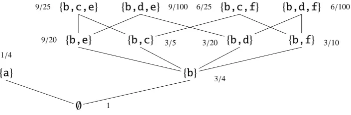
Fig. 2. An example of cell valuation and the probabilities of configurations
c ∈C, and then non-deterministically select (or probabilistically sample) an event e∈c. Update the current configuration by adding e.
The concept of cell-valuation formalises probabilistic sampling in cells. Here and in the following, for f : X → [0,+∞] a function and Y ⊆ X a set, we use f [Y] to denoteP
y∈Y f (y).
Definition 3.1 (Cell valuation, Varacca et al [23]) A cell valuation on a confusion-free event structure ES = (E,≤,#) is a function p : E → [0,1] such that for every cell c, we have p[c]=1.
If we assume (probabilistic) independence between events in cells, then we can compute the probability of any configuration x occurring simply as the product of the probabilities of the constituting events.
Proposition 3.2 ([23]) Let p be a cell valuation, and write p(x) forQ
e∈xp(e); then
• p(∅)= 1;
• p(x)≥ p(x0), if x⊆ x0;
• p(x)= p[C], if C is a maximal set of configurations covering x; • p is a probability distribution on maximal configurations.
In the formulation above, we say y covers x to mean y = x∪ {e}for some e. Observe that the implication of Proposition 3.2 is that p(x) must be interpreted as the probability that the (partial) configuration x is contained in the outcome of the computation. On maximal configurations, p yields a probability distribution. With reference to the event structure of our running example, the assignment
{a7→1/4; b7→3/4; c7→4/5; d7→1/5; e7→3/5; f 7→2/5}
4
A Bayesian framework for event-based models
As illustrated in the previous section, finding a cell valuation p : E → [0,1] is the key step to assign probabilities to the configurations of a finite, confusion-free event structure ES. Observe that to give one such p is to give for each cell c a func-tion pc : c →[0,1] with pc[c]= 1, i.e., a probability distribution. Our assumption
is, typical of the Bayesian approach, that the distributions pc exists independently
and immutably; our intention is, equally typical, for them to be ‘learned’ via exper-iments, that in our case means derived from the past history of interactions with an external entity. Under the following heading, we state explicitly the assumptions about the behaviour of entities in our model. We then proceed to (i) find abstrac-tions that preserve sufficient information under the model; and (ii) derive equations for predictive probabilities, i.e., formulae to answer questions such as “what is the probability of outcome x in the next interaction with entity q?”
4.1 The model
Let ES be a finite, confusion-free event structure ES and C(ES) = {c1,c2, . . . ,cM}
its set of its cells, where ci ={ei1, . . . ,eiKi}. We writeλDESfor the following assump-tions of our model:
each principal’s behaviour is so that there are fixed parametersΘci such that at each interaction there is, independently of anything we know about other interac-tions, probability distributionΘci for the events of cell cito occur, if ciis enabled. Such basic data are equivalent to give a probabilityΘeto each event e of ES, so that
PKi
k=1Θei
k = 1. The collectionΘ=(Θc1, . . . ,ΘcM) determines a cell valuation on ES. It follows from our assumption that for each configuration x∈ CES the probability of obtaining x in any run of ES with a principal parametrised byΘis
Prob(x|ΘλDES)=
Y
e∈x
Θe. (2)
In way of comparison with modelλBdescribed in§2,λDESassigns probabilities to (maximal) configurations to the same effect asλB does for the binary outcomes {s, f}. In this case however, the assignment is not ‘atomic,’ but obtained via a cell evaluation, i.e., an assignment of probability distributions to cells and, ultimately, to basic events. While the occurrence of an x from {s, f}is a binomial (Bernoulli) trial, the occurrence of an event from ci is a random process with Ki outcomes.
That is, a multinomial trial onΘci. To exploit this analogy, we therefore only need to lift the framework of§2 to one based on multinomial experiments. In particular, we shall need to identify a family of distributions that can play here the same role as theβ-distribution does there.
in force of Eq. (2), it is sufficient to estimate the parametersΘc for each cell c. It
then follows from the assumptions ofλDES that a count X of the event occurrences in h is the only significant information for any sequence h ∈ C∗
ES of data observed
about a fixed principal.
Secondly, in order to apply Bayesian analysis, we need prior distributions. As we intend to use our estimates to determine expected values for entire distributions, it is fundamental that we are able to compute them in symbolic form. This is one of the roles of conjugate priors. We phrase the following definition with terminology used in the Introduction to illustrate Bayes’ Theorem.
Definition 4.1 A family F of probability distributions is a conjugate prior for a likelihood function L if whenever the prior distribution belongs to F, then also the posterior distribution belongs to F.
Indeed, the use of conjugate priors generally affords a significant computational convenience in Bayesian analysis, in that the distributions always maintain the same algebraic form. As we shall see below, it turns out that the family of Dirichlet distributions is a family of conjugate prior distributions for multinomial trials.
The use of Dirichlet distributions as priors completes the picture of our appli-cation of Bayes’ Theorem to event structures. Specifically, a prior Dirichlet dis-tribution is assigned to each cell c of ES. Event counts X are then used to update the Dirichlet at each cell. Hence, at any time we have for each cell c a Dirichlet distribution on the parametersΘc of that cell. We will show that the probability of
an outcome x ⊆E is then the product of certain expectations of these distributions.
4.2 The Dirichlet distribution
The Dirichlet family D of order K, for 2 ≤ K ∈ N, is a parametrised collection of continuous probability density functions (pdf) defined on [0,1]K; K parameters of positive reals, α= (α1, . . . , αK), select a specific Dirichlet distribution from the
family. For a variableΘ = (Θ1, . . . ,ΘK)∈[0,1]K, the pdf is given by: D(Θ|α)= Γ(
P
iαi)
Q
iΓ(αi)
·YΘα1−1
1 · · ·Θ
αK−1
K ,
where the Gamma function, Γ(z) = R0∞tz−1e−tdt, for z > 0, is used to define the normalisation constant. Luckily, we shall not be explicitly concerned with such a constant. The main values of interests in our application are the expected value and the variance of variables distributed according to D(· | α) which, importantly, depend only onα. Namely, using [α] as a shorthand forP
jαj, we have:
ED(Θ|α)(Θi)=
αi
[α] σ
2
D(Θ|α)(Θi)=
αi([α]−αi)
4.3 A conjugate prior
Consider sequences of independent experiments with K-ary outcomes, each yield-ing outcome i with some fixed probability Θi; such experiments are multinomial trials (and in our framework correspond to the probabilistic choice of one event at a cell). Let λD denote a model collecting such hypothesis, and let Xi represent the ith trial (i =1, . . . ,n). In other words, Zi ≡ (Xi = ji) is the statement that the ith trial
has outcome ji ∈ {1,2, . . . ,K}. Let Z = (Z1, . . . ,Zn) be the conjunction of n such
statements. Then, by definition of multinomial trials, the sequence of independent experiments has the following likelihood:
Prob(Z |ΘλD)=
n
Y
i=1
Prob(Zi |ΘλD)= K
Y
i=1
Θ#i(Z)
i ,
where #i(Z) is the number of occurrences of i in Z.
The Dirichlet distributions constitute a family of conjugate prior distributions for this likelihood. In order to illustrate this fact, let us recall that according to Bayes’ Theorem one can derive from the prior distribution on Θ, say f (Θ | λD), and the experiments Z, a posterior distribution f (Θ| ZλD) as:
f (Θ|ZλD)= f (Θ| λD)
Prob(Z |ΘλD) Prob(Z |λD) .
In fact, it is not hard to show that when f (Θ | λD) is a Dirichlet distribution, say D(Θ|α1, . . . , αK), then f (Θ|ZλD) is a Dirichlet distribution too; viz.,
f (Θ|ZλD)= D Θ|α1+#1(Z), . . . , αK+#K(Z),
which is what we wanted. Note that by choosing αi = 1 for all i, the Dirichlet
distribution degenerates to the uniform distribution on [0,1]K. This is very useful, as it provides a convenient unbiased initial prior for those cases, relatively frequent in our application domain, where we have no prior information on principals. 4.4 Predictive probability in the Dirichlet modelλD
Let us now consider the statement Zn+1 ≡ (Xn+1 = i) before performing the n+1 experiment. We can then can interpret Prob(Zn+1 |ZλD) as a predictive probability: given no direct knowledge of Θ, but only past evidence (viz., Z) and the model (viz.,λD), then Prob(Zn+1 | ZλD) is the probability that the next trial will result in outcome i. It is easy to show that:
Prob(Zn+1 |ZλD)= Ef (Θ|ZλD)(Θi)=
αi+#i(Z)
[α]+n
Z. Then, given the Dirichlet expression above for f (Θ | ZλD) and the fact that
P
i#i(Z) = n, the results follows from the expectation formula (3). We remark
that the variance formula can be used at any time to evaluate the accuracy of our prediction: the lower the variance, the more likely the prediction.
4.5 Dirichlet distributions on cells
Returning to our event structure model, we will associate to each cell c ∈ C(ES) a Dirichlet prior distribution on the parameters Θc determining the behaviour of
a fixed principal for the events of c. As we interact with the principal, we use Bayes’ Theorem and the formulae derived above to tighten the parameters to the observation and therefore sharpen our ability to predict outcomes via the predictive probability. Each cell c ∈ C(ES) presents a choice between the mutually exclu-sive and exhaustive events of c, and by the assumptions ofλDES such choices are multinomial trials. At any time, we obtain the predictive probability of the next interaction resulting in a particular configuration by multiplying the expectations of the parameters for each event in the configuration.
Let us be precise. Let fc(Θc |λDES) denote the prior distribution for c∈C(ES), and let there be a positive real numberαe associated to each e∈E. We useαci as a shorthand for the vector of parameters associated to ci, i.e., (αei
1, . . . , αe
i
Ki). We are then just left with the task of adapting the formulae of§4.3. We have:
fci(Θci |λDES)=D(Θci |αci)=
Γ([αci])
QKi
k=1Γ(αei
k) ·
Ki
Y
k=1
Θαei k
−1
ei
k
.
Let X : E →Nbe an event count that models the observations about past runs with a specific principal. The posterior pdf is given below, where+denotes both scalar and vector sum, and X(ci)= (X(ei1), . . . ,X(eiKi)).
fci(Θci | XλDES)= D Θci |αci +X(ci)
= Γ([αci +X(ci)])
QKi
k=1Γ(αeik+ X(eik))
·
Ki
Y
k=1
Θαei k+
X(eik)−1
ei
k
.
Such fierce-looking formula is in reality very simple: it just states that each event count X : E → Ncan be used to do Bayesian updating of our cell valuation simply by adding X(e) toαe, for each e∈E.
4.6 Predictive probability in the modelλDES
Also in this case, we merely need to adapt the formulae derived in§4.4. Let X be an event count corresponding to the observation of n previous configurations x1· · ·xn
inλDES, the predictive probability Prob(Z | XλDES) is the product of the probabil-ities of occurrence of each e ∈ x. But the probability of ei
j occurring, provided its
cell ci is enabled, is exactly the expected value ofΘei
j, and since we know the pdfs fc(Θc |XλDES) for all c∈CES, we can use the expectation formulae (3).
E(Θei
j |XλDES)=
αei j +X(e
i
j)
α
ci +X(ci)
.
The predictive probability is therefore the product of the expectations of each of the cell parameters.
Prob(next outcome is x| XλDES)=Prob(Z |XλDES) = Y
e∈x
E(Θe |XλDES)=
Y
ei
j∈x
αei j +X(e
i
j)
α
ci + X(ci)
.
4.7 Summary
We have presented a probabilistic modelλDESbased on probabilistic confusion-free event structures. The model generalises previous work on probabilistic models us-ing binary outcomes and β prior distributions. In our model, given a past history with a principal we need only remember the event counts of the past, i.e., a function X : E →N. Given such an event count, there is a unique probability of any partic-ular configuration occurring as the next interaction. We have derived equations for this probability and it is easily computed in real systems.
With reference to the event structure of our running example, suppose we have the following event count X.
c: 7 /o /o d: 1 e : 3 /o /o f: 5
a : 2 /o /o /o /o /o /o /o /o /o /o /o /o /o b : 8
g
g
OOOOOOOOOOOO ooo77
o o o o o o o o o ] ] <<<<<< < A A
If we assume to start with uniform priors, i.e., αe = 1 for e ∈ {a,b,c,d,e,f},
then X gives rise to the following updated Dirichlet distributions. f{a,b}(Θa,Θb | XλDES)=D(Θa,Θb |3,9), f{c,d}(Θc,Θd | XλDES)=D(Θc,Θd |8,2), f{e,f}(Θe,Θf | XλDES)=D(Θe,Θf |4,6).
As an example, the probability of configuration{b,c}is Prob({b,c} | XλDES)=
In fact, the cell valuation arising from this is the one illustrated in Fig 2.
5
Towards a formal model of dynamic behaviour
In this section we reflect on what has been achieved in this paper, but mainly on what has not. Our main motivation when we started this investigation was to put on formal grounds what we had been seeing in the literature, so as to be able to ask sharp questions of our data. We succeeded in this to a comforting extent, both by presenting the first ever formal framework for the comparisons of computational trust algorithms and by extending a well-known formal concurrency model with a framework for Bayesian analysis.
However, while the purpose of models may not be to fit the data but to sharpen the questions, good models must do both! Our probabilistic models must be more realistic. For example, theβ-model of principal behaviour (which we consider to be state-of-the-art) assumes that for each principal p there is a single fixed parameter Θp so at each interaction, independently of anything else we know, the probability
of a ‘good’ outcome is Θp of the one of ‘bad’ outcome is 1 − Θp. One might
argue that this is unrealistic for some applications. In particular, the model allows for no dynamic behaviour, while in reality not only the p is likely to change its behaviour in time, as its environmental conditions change, but p’s behaviour in interactions with q is likely to depend on q’s behaviour in interactions with p. The same criticisms apply of course to the Dirichlet model we presented here.
Some beta-based reputation systems attempt to deal with the first problem by introducing so-called ‘forgetting factors.’ Essentially this amounts to choosing a factor 0 ≤ δ ≤ 1, and then each time the parameters (α, β) of the pdf for Θp are
updated, they are also scaled by δ. In particular, when observing a single ‘good’ interaction, (α, β) becomes (αδ+1, βδ) rather than (α, β). Effectively, this performs a form of exponential ‘decay’ on parameters. The idea is that information about old interactions is less relevant than new information, as it is more likely to be outdated. This approach represents a departure from the probabilistic beta model, where all interactions ‘weigh’ equally, and in the absence of any mathematical it is not clear what the exact benefits of this bias towards newer information is. Regarding the second problem, to our knowledge it has not yet been considered in the literature.
Let us point out some ideas towards refining such hypothesis and embracing the fact that the behaviour of p depends on its internal state, which is likely to change over time. Suppose we model p as a kind of Markov chain, a probabilistic finite-state system with n finite-states S ={1,2, . . . ,n}and n2transition probabilities t
i j ∈[0,1],
withPn
j=1ti j = 1. After each interaction, p changes state according to t: it takes a
transition from state i to state j with probability ti j. Such state-changes are likely
1
.01
+
+2
.25
k
k
π1=1 B1(a)=.95 B1(b)=.05
O={a,b}
[image:21.595.205.407.71.160.2]π2=0 B2(a)=.05 B2(b)=.95
Fig. 3. Example Hidden Markov Model.
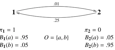
its interactions with p; based on that, it must make inferences on p’s likely state and future actions. If we accept the finite state assumption and the Markovian transition probabilities, we can then incorporate unobservable states in the model by using so-called Hidden Markov Models [19].
A discrete Hidden Markov Model (HMM) is a tuple λ = (S, π,t,O,s) where S is a finite set of states; π is a distribution on S , the initial distribution; t : S ×S → [0,1] is the transition matrix, withP
j∈S ti j = 1; finite set O is the set of possible observations; and where s : S ×O→[0,1], the signal, assigns to each state j∈S , a distribution sj on observations, i.e.,Po∈Osj(o)= 1.
An example. Consider the HMM in Figure 3. This models a simple two-state process with two possible observable outputs a and b. For example, this could model a channel which can forward a packet or drop it. State 1 models the normal mode of operation, whereas state 2 models operation under high load. Suppose that output a means ‘packet forwarded’ and output b means ‘packet dropped.’ Most of the time, the channel is in state 1, and packets are forwarded with probability
.95; occasionally the channel will transit to state 2 where packets are dropped with probability.95. Although this example is just meant to illustrate a simple HMM, we expect that by tuning their parameters Hidden Markov Models can provide an interesting model many of the dynamic behaviours needed for probabilistic trust-based systems.
Consider now an observation sequence, h = a10b2 (that is ten a’s followed by two b’s), which is reasonably probable in our model on Figure 3. The final fragment consisting of two consecutive occurrences of b’s makes it likely that a state-change from 1 to 2 has occurred. Nevertheless, a simple counting algorithm, sayH, would probably assign high probability to the event that a will happen next:
H(a|h)= #a(a
10b2)+1
|h|+2 = 11/14∼ .80
However, if a state-change has indeed occurred, that probability would be as low as.05.
quickly, and assign probability H(a | h) ∼ .25, which is a much better estimate. However, suppose that we now observe bb and then another a. Again this would be reasonably likely in state 2, and would make a state-change to 1 probable in the model. The exponential forgetting would assign a high weight to a, but also a high weight to b, because the last four observations were b’s. In a sense, perhaps the algorithm adapts ‘too quickly,’ it is too sensitive to new observations. So, no matter whatδis, it appears easy to describe situations where it does not reach its intended objective; our main point here is the same as for our comparisons of computational trust algorithms in§2: that the underlying assumptions behind a computational idea (e.g., the exponential decay) need to be specified, and that formal models for prin-cipal’s behaviour (e.g., HMMs) may serve the purpose, allowing precise questions on the applicability of the computational idea.
6
Conclusion
Our ‘position’ on computational trust research is that any proposed system should be able to answer two fundamental questions precisely: What are the assumptions about the intended environments for the system? And what is the objective of the system? An advantage of formal probabilistic models is that they enable rigorous answers to these questions. To illustrate the point, we have presented an example of a formal probabilistic model, λDES. The central technical contribution here has been to recast one of the best known and most popular models of concurrency, the event structures, in a framework for Bayesian analysis. This allows ‘learning’ and ‘prediction’ of composite, multi-event structured outcomes (viz., event structure configurations) in complex interaction protocols (viz., event structures). We antic-ipate the model will be useful in several applications, even though in the paper we discussed some of its shortcomings and hinted at future developments.
Among the several benefits of formal probabilistic models, we have focussed on the possibility to compare algorithms, sayX andY, that work under the same assumption on principal behaviours. The comparison technique we proposed relies on Kullback and Liebler’s information diverge, and consists of measuring which algorithm best approximates the ‘true’ principal behaviour postulated by the model. For example, in order to compareXandYin the modelλ, we propose to compute and compare
DnKL(λk X) and DnKL(λk Y).
Θ, there exists a best approximating algorithm. Remarkably, this does not depend on n, the length of the training sequence. We regard this as the main result of the paper. More generally, another type of property one might desire to prove using the notion of information diverge is that limn→∞DnKL(λ k X) = 0, meaning that algorithm X approximates the true principal behaviour to an arbitrary precision, given a sufficiently long training sequence.
References
[1] M. Blaze, J. Feigenbaum, J. Ioannidis, and A. D. Keromytis. The role of trust management in distributed systems security. In Jan Vitek and Christian D. Jensen, editors, Secure Internet Programming: Security Issues for Mobile and Distributed Objects, volume 1603 of Lecture Notes in Computer Science, pages 185–210. Springer, 1999.
[2] S. Buchegger and J-Y. Le Boudec. A Robust Reputation System for Peer-to-Peer and Mobile Ad-hoc Networks. In P2PEcon 2004, 2004.
[3] V. Cahill and E. Gray et al. Using trust for secure collaboration in uncertain environments. IEEE Pervasive Computing, 2(3):52–61, 2003.
[4] V. Cahill and J-M. Seigneur. The SECURE website. http://secure.dsg.cs.tcd. ie, 2004.
[5] D. Chalmers, M. Chalmers, J. Crowcroft, M. Kwiatkowska, R. Milner, E. ONeill, T. Rodden, V. Sassone, and M. Sloman. Ubiquitous computing: Experience, design and science. Version 4. Available from:http://www-dse.doc.ic.ac.uk/
Projects/UbiNet/GC/Manifesto/manifesto.pdf, 2006.
[6] K. Chatzikokolakis, C. Palamidessi, and P. Panangaden. Anonymity protocols as noisy channels. In Proceedings of TGC’06, LNCS. Springer, 2007. To appear.
[7] Z. Despotovic and K. Aberer. A probabilistic approach to predict peers’ performance in P2P networks. In Proceedings from the Eighth International Workshop on Cooperative Information Agents (CIA 2004), volume 3191 of Springer Lecture Notes in Computer Science, pages 62–76. Springer, 2004.
[8] Z. Despotovic and K. Aberer. P2P reputation management: Probabilistic estimation vs. social networks. Computer Networks, 50(4):485–500, Mar. 2006.
[9] D. Gambetta. Can we trust trust? In Diego Gambetta, editor, Trust: Making and Breaking Cooperative Relations, pages 213–237. University of Oxford, Department of Sociology, 2000. Chapter 13. Electronic edition http://www.sociology.ox.
ac.uk/papers/gambetta213-237.pdf.
[11] A. Jøsang and J. Haller. Dirichlet reputation systems. In Proceedings of the 2nd Intl Conference on Availability, Reliability and Security, ARES 2007. 2007. To appear.
[12] A. Jøsang and R. Ismail. The beta reputation system. In Proceedings from the 15th Bled Conference on Electronic Commerce, Bled, 2002.
[13] K. Krukow. Towards a Theory of Trust for the Global Ubiquitous Computer. PhD thesis, University of Aarhus, Denmark, August 2006. ; available online (submitted):
http://www.brics.dk/˜krukow.
[14] K. Krukow, M. Nielsen, and V. Sassone. A logical framework for reputation systems. Journal of Computer Security, 2007. To appear. Available online www.brics.dk/ ˜krukow.
[15] S. Kullback and R.A. Leibler. On information and sufficiency. Annals of Mathematical Statistics, 22(1):79–86, March 1951.
[16] L. Mui, M. Mohtashemi, and A. Halberstadt. A computational model of trust and reputation (for ebusinesses). In Proceedings from 5th Annual Hawaii International Conference on System Sciences (HICSS’02), page 188. IEEE, 2002.
[17] M. Nielsen and K. Krukow. On the formal modelling of trust in reputation-based systems. In J. Karhum¨aki, H. Maurer, G. Paun, and G. Rozenberg, editors, Theory Is Forever: Essays Dedicated to Arto Salomaa on the Occasion of His 70th Birthday, volume 3113 of Lecture Notes in Computer Science, pages 192–204. Springer Verlag, 2004.
[18] M. Nielsen, G. Plotkin, and G. Winskel. Petri nets, event structures and domains. Theoretical Computer Science, 13:85–108, 1981.
[19] L.R. Rabiner. A tutorial on hidden markov models and selected applications in speech recognition. Proceedings of the IEEE, 77(2):257–286, February 1989.
[20] S. Reece, A. Rogers, S. Roberts, and N. Jennings. Rumours and reputation: Evaluating multi-dimensional trust within a decentralised reputation system. In Proceedings of the 6th Intl Joint Conference on Autonomous Agents and Multiagent Systems, AAMAS-07. 20AAMAS-07. Available athttp://eprints.ecs.soton.ac.uk/13260.
[21] J. Sabater and C. Sierra. Review on computational trust and reputation models. Artificial Intelligence Review, 24(1):33–60, 2005.
[22] W.T.L. Teacy, J. Patel, N.R. Jennings, and M. Luck. Coping with inaccurate reputation sources: experimental analysis of a probabilistic trust model. In AAMAS ’05: Proceedings of the fourth international joint conference on Autonomous agents and multiagent systems, pages 997–1004, New York, NY, USA, 2005. ACM Press.