City, University of London Institutional Repository
Citation
:
Mayhew, L. and Smith, D. (2009). Whither human survival and longevity or the shape of things to come (Actuarial Research Paper No. 189). London, UK: Faculty of Actuarial Science & Insurance, City University London.This is the unspecified version of the paper.
This version of the publication may differ from the final published
version.
Permanent repository link:
http://openaccess.city.ac.uk/2320/Link to published version
:
Actuarial Research Paper No. 189Copyright and reuse:
City Research Online aims to make research
outputs of City, University of London available to a wider audience.
Copyright and Moral Rights remain with the author(s) and/or copyright
holders. URLs from City Research Online may be freely distributed and
linked to.
City Research Online: http://openaccess.city.ac.uk/ [email protected]
Faculty of Actuarial
Science
and
Insurance
Actuarial Research Paper
No. 189
Whither Human Survival and Longevity
or
The Shape of Things to Come
Leslie Mayhew and David Smith
June
2009
Cass Business School
106 Bunhill Row
London EC1Y 8TZ
Tel +44 (0)20 7040 8470
Whither Human Survival and Longevity
or
The Shape of Things to Come
Contents
1.
Introduction
2.
Modelling approach and basic ideas
3.
The empirical model
4.
Developing projections
5.
Future projections
6.
Conclusions
References
Annexes
Author email addresses
Whither Human Survival and Longevity
or
The Shape of Things to Come
Leslie Mayhew and David Smith
Faculty of Actuarial Science and Insurance Cass Business School
Abstract
With the continuing increases in life expectancy, populations are ageing rapidly. Governments are concerned for the future of pensions and health care for which population forecasts are an important component for planning purposes. In this paper we focus on human survival rather than mortality rates which are the more usual starting point when estimating future populations. Using a simple model we link basic measures of life expectancy to the shape of the human survival function and consider its various forms. We then use the simple model as the basis for investigating actual survival in England and Wales from 1841 onwards and investigate the concept of a ‘maximum age’. We show how the model can be used in a predictive sense and demonstrate in two tests that show our model would have given more accurate results than comparable government forecasts using the same base information. We then go on to show that, based on trends in life expectancy, official population forecasts could undershoot the population at age 50+ by 0.6m, with consequent financial implications for pensions, health and social care.
1. Introduction
In June 2009 Henry Allingham of the UK celebrated his 113th birthday, one of a tiny number of people that have made it to such an old age. On present trends the next 20 years or so will see a six fold increase in the number of centenarians in this country to around 60,000 and so Henry Allingham will potentially be joined by many others, not only in the UK but also around the world (Manton et al, 1991; Coale, 1996; Vaupel, 1998; Wilmoth and Robine, 2003; Robine and Saito, 2003).
However, amidst the celebrations of his achievement it is still the case that around 14% of English males will die before their 65th birthday and 31% before their 75th birthday. The highly publicised increases in life expectancy have thus to an extent masked the fact that life span is still hugely variable even in prosperous countries.
We have reached the present position in which the majority of UK citizens live until they are at least 80 years old as a result of many factors and influences spread over 100 years. These include massive reductions in childhood mortality through better nutrition and immunisation programmes that has led to mortality under 30 years of age virtually disappearing, better welfare safety nets leading to poverty reduction, improved health care, central heating, more recently life style changes from reductions in smoking, and finally better treatment and management of chronic diseases in old age particularly heart disease.
Nevertheless, inequality in life span is arguably the most fundamental inequality that exists among human populations (Rogers, 1995; Carey, 2003; Edwards and Tuljapurkar, 2005; Wachter, 2003) and so progress in reducing it is of significant interest in public policy terms. For example the UK government target is to reduce health inequalities by 10% by 2010 as measured by infant mortality and life expectancy at birth between the worst performing areas of the UK and the rest. To what extent is the achievement of this target supported by trends in S(x), the proportion of the population surviving to age x, through time and by when is it likely to be accomplished?
Such changes in the way we live spread over many years, prompts a number of questions. For example, whether inequalities are reducing or increasing through time, or whether there are upper limits to life span or if patterns differ between countries, in particular those at different stages of economic development or with different cultures. An interesting question for example is whether countries experiencing rapid development and economic growth exhibit similar patterns in human survival to already developed countries, and if there are differences whether they are attributable to differences in governance or approaches to welfare.
The literature on the subject of human survival is considerable, going back in some cases centuries (Olshansky and Carnes, 1997). Among the many papers on the subject, Fries (1980) made the important observation that, although more people were living longer for all these reasons, the shape of the human survival curve S(x) was becoming more rectangular in shape, suggesting that there were possible biological limits to life span.
This has sparked considerable debate in the literature ever since in which the arguments broadly resolve into two camps. One agrees with Fries which is that from a rational standpoint there must be biological limits to life expectancy and it is only a matter of ‘when’ and not ‘if’ they limit is reached. The other camp points to the fact that there has been an unbroken linear rise in life expectancy of about three months a year for at least 150 years and that there are no signs of this abating (Oeppen and Vaupel, 2006). In the leader board of life expectancies in different countries, the position has changed many times over the years with, for example, New Zealand in the first half of last century leading the way, then Scandinavia, briefly Switzerland, and now Japan. Supporters of this viewpoint hence argue that, taking the world as a whole, it is premature to talk of upper limits for so long as this trend persists.
and Horiuchi. 1999; Kanisto, 2000; Lynch and Brown, 2001). Their ultimate focus is on the ‘compression of human mortality’ and around an upper limit to life span rather than on the driving forces. Edwards and Tuljapurkar (2005), using the Kulber-Leibler divergence to compare changes over time, found evidence of differences in S(x) according to socio-economic inequality, associated factors such as educational status and ethnicity as well as for example gender.
For an actuary, pension provider or health economist, maximum life span is arguably mainly of academic interest as compared with S(x). The reason is that very few people will reach the maximum life span while changes in the numbers of people reaching different ages will determine the future benefits to be paid out in the case of life assurance and pension provision, and will inform the demand for social security and health care from the public purse. Such information is customarily supported by official published population projections. A problem is that there has been a tendency to under-estimate improvements in mortality especially at older ages, resulting in population forecasts that are too low (Bengtsson, and Keilman, 2003).
In this paper we will argue that there is very little sense of overall strategic direction or indication of speed of change in human survival, so that we do not know if this year’s projections will alter significantly from one year to the next or how this will affect future planning assumptions. An example of this would be the answer to the question of how far pension age should be raised, and if life expectancy increases faster than we had planned for in our calculations, how many more people will survive to pensionable age than we had anticipated? A simple look-up table or chart may be more practicable in this regard than repeated model runs of different population scenarios (Blake and Mayhew, 2006).
Taking these considerations into account, measures of rectangularistion do not directly lead to the answer of how many people will survive to age x between now and 2020 and nor how many deaths would be avoided as a result each year in the intervening period. What would be helpful are methods to predict the shape of S(x) going forward from which can be derived many useful measures including how many lives will survive to any given age. To do this we need to understand patterns of survival in more detail.
In this paper we develop a model that builds on regularities in the survival curve to shed light on some of these important questions, whether life expectancy is measured at birth or at any other age. The paper has five objectives; they are to:
- model and predict changes in the shape of the survival curve through time so that for example knowing where life expectancy will be in the future will enable accurate estimates of the percentages surviving to different ages
- use the model to investigate whether there is evidence of a human ‘maximum’ age and, if so, how many years will elapse until that point is reached
- estimate how many extra lives will be saved each year and at which ages as survival rates improve
- test whether the approach produces more accurate estimates of survivorship than currently used methods that spring from mortality models in the first instance.
We use data for England and Wales concentrating on the period 1841 to 2003 to illustrate or findings. First, however, we outline the modelling approach and develop the mathematical framework we need to develop the basics ideas used in the analysis. Later sections apply the model to historical data to interpret the past and as a basis for building projections in which technical details on how projections are constructed are included. Since survival is the converse of death, the method is theoretically complementary to customary methods based on projecting mortality rates although differences arise due to technical differences of approach.
Limitations of space restrict the number of empirical examples that can be provided in this paper, although we have tested the method on data from several countries. In presenting our results, we consider the case of predicting survivorship from 1981 to the present using then GAD forecasts and our forecasts based on the model but from a 1981 perspective and then with a similar procedure for 1991. We then compare the performance of both models with the realised survivorship rates and compare what happens when the model is rolled forward to 2020. A concluding section reflects on the principal findings and overall approach and discusses follow-on work.
The origins of the techniques described are derived from research in two other unrelated fields both of which use queuing theory. These are worthy of mention because they illustrate a commonality of mathematical processes under different guises that suggests, in turn, a range of other possible applications. The first of these is described in Mayhew (1987) which is concerned with estimating the time elapsed by social security claims in the system and was used for setting social security targets, and the second is based on time to discharge times in accident and emergency departments (Mayhew and Smith, 2007). Both in fact have their basis in types of survival curve, but the distributions are known by different names in the queuing literature (usually the distribution of ‘time spent in the system’).
The fact that in both cases there are statistically robust empirical regularities between average time spent and the time taken to process a given percentage of social security claims or patients in an A&E department encouraged us to believe that similar regularities are observable in other fields, in this case human survival. Such an example is given in Mayhew (2001) which investigates the issue of long term care provision in Japan. Trends in life expectancy are used to project the Japanese survival curve in future years and hence the numbers of people likely to need long term care going forward. The key difference is that sojourns in these environments are ideally as short as possible but in life most want to remain in the system as long as possible ~ a life in slow lane!
o There has been a fundamental change in the pattern of survivorship from 1946 with the result that previously indicated trends of a convergence in survival ages has stalled. At the oldest ages the survival ages are becoming more divergent with no sign of slowing down so that some people will live ever longer. These and other findings could mean that the Government target of reducing health inequalities which relies on a convergence in life expectancy in different areas of the country may not be achievable.
o The underlying model that generates these patterns and trends, described in the first part of the paper, can be adapted to produce future life tables that appear to be more accurate than those officially used as the basis for population projections. This finding is based on a comparison of our model with GAD projections made in 1981 and 1991 and comparing the results with what actually occurred.
o In projecting forward to 2020 our model shows greater survivorship than official GAD forecasts suggesting that there will be even higher numbers of older people than is currently being planned for. For example using 2001 as our base year we estimate that the number of males aged 50+ in 2020 will be approximately 0.7m higher than GAD’s own principal 2001 based projection for 2020. If correct this finding has implications for pensions, life insurance and services for older people such as health and social care that rely on population projections for planning and distribution purposes.
2. Modelling approach and basic ideas
Mathematically the survival curve denoted by S(x) denotes the probability of surviving to age x whereas e(x) defines life expectancy at age x. With no loss of generality we initially develop our ideas into the form of a simple, stylised model in order to gain insights into the processes linking survival and life expectancy. This allows us to derive a basic relationship between the survival processes and simple dynamics that allow us to estimate lives saved, and mortality at different ages.
To calibrate the model in practice we use a form of the conventional Gompertz-Makeham survival curve in order to investigate the actual relationship between lives saved at different ages over time. However, we do not place restrictions on the values that the parameters are able to take. By exploiting the regularities in the data and trends over time we are also able to make a qualified guess at whether populations are converging towards a maximum life span, how many lives are saved each year of life expectancy, and the speed at which the survival curve is converging or otherwise.
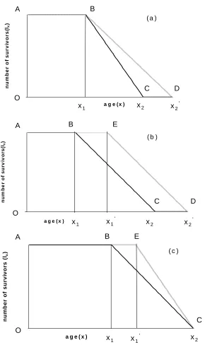
Imagine a stationary population in which there is a constant number of births and deaths, no migration and which is subjected to the same mortality regime each year. Consider Figures 1(a) – (c), which show the mortality curves ABC for three such hypothetical populations at a given point in time. The vertical axis shows the number of survivors lx and the horizontal axis age x. We define the point x1 in each case as the
Figure 1: Three hypothetical mortality models (a), (b) and (c)
Both x1 and x2 are somewhat fuzzy quantities in the real world. In developed
countries we could assume the onset of mortality (x1) occurs from around 50 years onwards. Alternatively this may be defined by reference to particular percentile of deaths, for example 10%, to remove the effects of accidents and rare diseases that affect few of the population. Similarly, rather than look at the final death in a population it may be more appropriate to assume that x2 is the age of death of the 90th percentile. However, our purpose is to use them as conceptually useful devices to anchor and compare distributions and mortality processes rather than to determine them empirically.
0
0
a g e ( x )
nu
m
b
er
of
s
u
r
v
iv
or
s(
lx
)
A B
D C
x1 x2 x2'
O
( a )
0 0
a g e ( x )
num
be
r of
s
u
rv
iv
or
s
(lx
)
x1' x2 x2'
x1
A B
C D
E
( b )
O
0 0
a g e ( x )
n
u
mb
er
of survi
vors (l
x
)
A B E
C x1 x1' x2
O
Now imagine the age distribution of the population at another point in time. In model (a), we see that x1 is unchanged whilst x2 the oldest age has advanced to x2′ (point D). In other words the onset of mortality is unchanged but now some people live to older ages. The consequence of this is a decline in the mortality gradient BD compared with BC. In model (b) we see that both x1 and x 2 have advanced by the same amount, such that the mortality gradient is the same before and after. In model (c) x2 has remained constant but x1 has advanced to x1′ (point E) with the effect that
the mortality gradient is steeper. For reasons that will become apparent shortly we call (a) the dispersed mortality model, (b) the parallel mortality model and (c) the compressed mortality model
What do the models tell us about the evolution of populations following one or other of these evolutionary paths? Qualitatively speaking, model (a) might be thought of benefiting older people more than younger people, model (b) all age groups equally and model (c) younger generations before older generations.
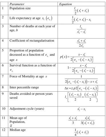
Some relationships and properties of the simple model
Table 1 is a list of basic parameters comparing each of the three models. Assume the number of survivors at a given age is lx. Line 1 in the parameter list (table 1) shows
the population for each case as a function of x1and x2. This is simply the area under
the population curve. Line 2 shows life expectancy
1
x
e at x1 as a function of x1 and
2
x . Line 3 shows the mortality gradient or number of deaths at each age where death can occur. As shown, this value must increase if the difference between the age when people start dying and the age at which all lives have ceased decreases. This is to ensure a stable population as an increase in the number of deaths at each age is needed so that total deaths are the same.
Line 4 is a measure of the degree to which the mortality curve is rectangular in shape, following Wilmoth and Horiuchi (1999). The nearer the ratio is to one the closer the mortality curve is to a rectangle. It is calculated by comparing the area under the mortality curve from birth with the encompassing rectangle whose base ranges from the age at which mortality age to x2.
Line 5 shows the theoretical relationship between cumulative mortalityp x
( )
, life expectancy at x1and a specified age, x, that is greater thanx1. These equations are most easily understood in the context of Figure 2a-c. Figure 2a depicts the dispersion case in which x1 is assumed fixed while x2 increases. On the vertical axis is lifeone-year advance in life expectancy at x1 translates into 2 extra years in maximum age as can be easily verified.
Parameter Mortality dispersion (A)
Parallel Mortality (B) Mortality compression (C)
1 Population size
(
)
1 2
2 x l
x +x′
(
1 2)
2 x l
x′+x′
(
1 2)
2 x l
x′+x′
2 Life expectancy at age x1
( )
1
x
e 2( )
1
1 ' 2 x
x − 1
(
1 2)
12 x′+x′ −x
(
1 2)
1 12 x′ +x −x 3 Number of deaths
at each year of age where death is possible
1
2 1
x l
x′ −x
1
2 1
x l
x′−x′
1
2 1
x l
x −x′
4 Coefficient of rectangularisation 2 1 2 2 x x x ′ +
′ 22 2 1
x x
x
′+ ′
′ 22 2 1
x x
x
′ +
′
5 Proportion of population deceased as a function of
1
x e and
age x
( )
1 1 2 x x x p x e − =( )
(
)
(
1)
1
1 1
2 x
x x p x
e x x
′ − = ′ − −
( )
(
(
)
)
1 1 1 1 2 x x x p xe x x
′ − =
′
− −
6 Survival function as a function of
1 x e 1 1 1 2 x x x e − −
(
)
(
1)
1
1 1
1 2 x
x x e x x
′ − − ′ − −
(
(
)
)
1 1 1 1 1 2 x x x e x x′ − −
′
− −
7 Force of Mortality at age x
1 1
1
2ex − +x x
(
(
)
)
1 1 1 1
1
2 ex − x′−x − +x x′
(
(
)
)
1 1 1 1
1
2 ex − x′−x − +x x′
8 Inter percentile
range, Δx 1
( )
2exΔp x 2(ex1+ −x1 x1′)Δp x( )
(
)
( )
1
2 1
2 x − −x ex Δp x
9 Deaths avoided or
person years saved 1
(
2 2)
2 x l
x′ −x lx1
(
x2′ −x2)
1(
)
1 1
2 x l
x′ −x 10 Adjustment cycle
(years)
2 1
x′ −x x2′ −x1 x2−x1
11 Mean age of
Population, x
(
)
1 2 1 2 1 2
3 3
x x x x x x ′ ′ + − ′ +
(
)
1 2 1 2 1 2
3 3
x x x x x x
′+ ′ ′ ′
−
′+ ′
(
)
1 2 1 2 1 2
3 3
x x x x x x
′+ ′
− ′ +
12 Median age
(
)
1 2
1
4 x +x
(
1 2)
14 x′+x′
(
1 2)
1
Figure 2: Cumulative mortality for each case: (a), (b) and (c)
In Figure 2b we have the same axes as before but cumulative mortality is now assumed to be parallel; that is to say each advance in life expectancy has exactly the same proportional effect on the chances of survival at all ages above the given age
25 30 35 40 45 50
50 60 70 80 90 100 110
age li fe exp ect an cy at ag e 50 ( e50 ) 0% 10% 20% 30% 40% 50% 60% 70% 80% 90% 100% 0 10 20 30 40 50
50 60 70 80 90 100 110
age li fe exp ec ta n cy at ag e 50 ( e50 )
0% 10% 20% 30% 40% 50% 60% 70% 80% 90% 100% 25 30 35 40 45 50
50 60 70 80 90 100 110
and so all age groups appear to benefit equally. To aid the illustration x1 is again
initially set to 50 and x2 to 100, where both parameters are assumed to advance in lock step. Minimum life expectancy in this case is 25 years rising to an assumed maximum of 50 years, which is why the vertical axis starts at 25 and not 0 as in case (a). Now only the 0% mortality curve passes through the origin, whereas previously all the percentiles did so. As for this model, the increase in values for x1 and x2 must
be the same value, each one-year increase in life expectancy advances both x1 and x2 by one year, as can be easily verified.
In 2c cumulative mortality from 50 converges to a point as x1 advances while x2 is held constant. As with case (b), minimum life expectancy at 50 is 25 years assuming
1
x equals 50 and x2 equals 100. Similarly, only the 0% mortality curve passes
through the origin, but note that the lines meet when the onset of mortality x equals 1
the maximum age x2. Life expectancy at this point is given by x2−x1so for example if x 2 equals 100 and x1 equals 50 the maximum life expectancy is 100-50=50. In
other words all people live to 100! Since x2 is fixed each one-year advance in life
expectancy equates to a 1-year delay in the onset of mortality,x1, up to a maximum of
2
x , and so the rate at which the lines converge depends on advances in life expectancy.
It is noteworthy that the median age (denoted by the 50th percentile) is identical in all three models with a cumulative mortality gradient of one. This can be seen by putting
( )
0.5p x = in each equation in line 5 and simplifying to give
1 1
x
e = −x x in each case. Put another way, it means that a one-year increase in life expectancy always equates to a rise in median age of one year regardless of which model one uses.
Line 6 shows the survival function as a function of
1
x
e . This is simply 1 less the
proportion of lives that have died as stated in line 5.
Line 7 shows the force of mortality calculated using
( )
( )
( )
d S x dx x
S x
μ =−
So for the Mortality Dispersion Model:
( )
(
)
(
)
{
}
(
)
(
)
{
}
(
)
(
)
1 1 1 1 1 1 1 1 1 1 11 1 1
1
1
1 exp
2
exp ln 2
exp ln 2 ln 2
2 exp ln 2 1 2 x x x x x x x x x x x
S x dt
e t x
e t x
e x x e x x
e x x
e x x e ⎧ ⎫ ⎪ ⎪ = ⎨− ⎬ − − ⎪ ⎪ ⎩ ⎭ ⎡ ⎤ = ⎣ − − ⎦ ⎡ ⎤ ⎡ ⎤ = ⎣ − − ⎦− ⎣ − − ⎦ ⎧ ⎡ − − ⎤⎫ ⎪ ⎪ = ⎨ ⎢ ⎥⎬ ⎢ ⎥ ⎪ ⎣ ⎦⎪ ⎩ ⎭ − = −
∫
Wilmoth and Horiuchi (1999) noted the degree of convergence (or divergence) in mortality curves provided one possible measure of rectangularisation, and suggested the age difference between the inter-quartile range for this purpose. In line 8, we generalise this concept and call it the inter-percentile range. Consider model (a) and assume the inter-percentile range is 0.8 i.e. (90%-10%) and that life expectancy at x1 is 20 years. The Inter-percentile age range is 2 20 0.8× × or 32 years but if life expectancy is 30 years the range is 48 years or 50% larger.
If we now consider model (b) the IPR is, not surprisingly, constant for any given value of life expectancy. For example, if
1 1 1
2(ex + −x x′) 10= , i.e. the expectation of life at age x1′ is 10 years, and the IPR is 0.8 then the age range would be 8 years. In
the convergent case, it is obvious from Figure 2c the IPR reduces as life expectancy increases. Plugging similar numbers into model (c) as before and assuming a maximum age x2 equal to 100 then when life expectancy is 40 we obtain an IPR of 16 (calculated as 2 0.8 (100 50 40)× × − − ) and similarly an IPR of 48 years when life expectancy is 20 years. The line arrow in Figure 2c denotes this case.
On some more general points we note that the derivative or slope of the cumulative
mortality curves
1
x d
e
dx is independent of both x1 and x2. This means that changes in these parameters will not affect the general shape of the graphs, but they will cause a scale shift on the horizontal and vertical axes. It is further evident that the slopes in models (a) and (c) are functions of pwhereas in model (b) the slope is a constant, as noted above. It is normally assumed that mortality rates decline in old age. In our
models age specific mortality rates are given by
2
1
Of the three models, it is readily apparent that (c) comes closest to the model originally proposed by Fries (1980). This because it is the only case among the three in which the coefficient of rectangularization (line 4) converges to a value of one, which occurs when x1equalsx2. The other two models approach a value of one but
only as x2′ becomes unrealistically large. Since rectangularization has been thoroughly studied by Wilmoth and Horiuchi (1999), we do not pursue it further here but simply note the range of outcomes.
Population Size
The table shows there are different equations for the three distinct models. However this does not need to be the case, as all models have anx1′ and anx2′, it is just that the value is sometimes the same as the original. If we are happy to allow the situation where x1′ =x1or x2′ =x2then we can have one equation for all three models: e.g.
Population size = 2 1 2 1 1
( ) ( )
2 2
x x x
x x x x
l x′ +l ′− ′ =l ′+ ′
Similarly, by using ‘new’ values for all models we are able to get life expectancy to always equal
(
2 1) (
1 1)
(
2 1)
11 1
2 x′−x′ + x′−x =2 x′+x′ −x
As the population is assumed to be stationery the total number of deaths per year must equal lx. Therefore the number of deaths at a particular age, where this age must be
greater than x1′ , can always be expressed as:
1
2 1
x l
x′ −x′
In terms of the degree of rectangularisation , we have
Area of rectangle = l xx 2′
Area under mortality curve = 1 1
(
2 1)
1(
2 1)
2 2
x x x
l x′+ l x′ −x′ = l x′ +x′
Co-efficient =
(
2 1)
2 12 2
2 2
x
x
l x x x x
l x x
′+ ′ ′ + ′ =
′ ′
The proportion of population deceased as a function of
1
x
e and age xis then,
(
)
1
1 1
1
2 1 1 1
where 2 x
x x x x
x x x x e x x
′ ′
− − ′
= ≥
′ − ′ ⎡⎣ − ′− ⎤⎦
(
2 1)
2 x1(
1 1)
p x′ −x′ = p ⎡⎣e − x′−x ⎤⎦
+ +
By general reasoning the increase in the stationary population must be the lives saved over the period.
(
2 2) (
1 1)
2 2
x
x x x x l ⎡⎢ ′ − + ′− ⎤⎥
[image:17.595.113.484.222.702.2]⎣ ⎦
Table 1 can therefore be simplified to:
Parameter Equation
1 Population size
(
)
1 2
2 x l
x′+x′
2 Life expectancy at age
1
x
( )
1
x
e
(
)
2 1 1
1
2 x′+x′ −x 3 Number of deaths at each year of
age, b 1
2 1
x l
x′ −x′
4 Coefficient of rectangularisation 2 1
2 2 x x x ′ + ′ ′
5 Proportion of population deceased as a function of
1
x e and
age x
( )
(
)
1 1 1 1 2 x x x p x
e x x
′ − =
⎡ − ′− ⎤
⎣ ⎦
6 Survival function as a function of
1
x
e
(
)
1 1 1 1 1 2 x x x e x x
′ − −
⎡ − ′− ⎤
⎣ ⎦
7 Force of Mortality at age x
(
)
(
1 1 1)
11
2 ex − x′−x − +x x′
8 Inter percentile range
(
)
1 1 1
2 x
x p ⎡e x′ x ⎤
Δ =+ ⎣ − − ⎦
9 Deaths avoided or person years
saved
(
2 2) (
1 1)
2 2
x
x x x x l ⎡⎢ ′− + ′− ⎤⎥
⎣ ⎦
10 Adjustment cycle (years) x2′ −x1
11 Mean age of Population,
a
(
)
1 2 1 2 1 2
3 3
x x x x x x
′+ ′ ′ ′
−
′+ ′
12 Median age
(
)
1 2
1
Mortality Rates
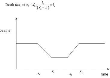
We need to understand how populations adjust to changes in mortality prospects for subsequent cohorts through time in order to assess the impact of improved survival on the lives saved at each age. Again we adopt a simplified approach, by considering each of the models separately and then bring them together in a rather clumsy general equation.
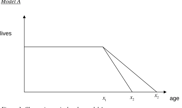
[image:18.595.88.467.187.413.2]Model A
Figure 3: Change in survival under model A
If we consider a particular year where the population suddenly become ‘healthier’ i.e. they are the first people to have the potential to reach agex2′, then we need time to elapse until they reach the age x1.
For t≤x1 i.e. before these new ‘healthier’ lives reach x1
Death rate
(
) (
)
2 1
2 1
x
x
l
x x l
x x
= − =
−
This is of course intuitive as we start with a stable population and if lx people are born then the same number must die.
Forx1< ≤t x2 i.e. when the new ‘healthier’ lives reach x1and die at the new lower rate
but we still have some older lives dying at the original rate
Death rate
(
) (
) (
) (
)
2 1
2 1 2 1
x x
l l
x t t x
x x x x
= − + −
′
− −
The first term involves the older lives who die at the original rate. As t increases this number reduces (as the population with original mortality rates dies out). The second
1
x x2 2
x′ lives
term involves the newer lives dying at the newer, lower rate. As t increases the value of this term increases as a larger number of people from this population reach ages where they can die. The overall death rate decreases as t increases over this range of values. The population is therefore growing over this period and growth reaches a maximum at time t=x2.
For x2 < ≤t x2′ i.e. all the older lives have died off but no new lives have yet reached the new maximum age x2′ i.e. the population is still increasing.
Death rate
(
) (
)
1
2 1
x
l t x
x x
= −
′ −
As there are only new lives left we only have the new death rate but we haven’t reached the stable population yet. As t increases the number of people in the total population and the population exposed to mortality increases and the number of deaths also increases.
Forx2′ <t i.e. the new maximum age has been reached and the population is again stable
Death rate
(
) (
)
2 1
2 1
x
x
l
x x l
x x
′
= − =
′ −
[image:19.595.94.499.353.709.2]Deaths under model A
Figure 4: Deaths under model A
1
x x2 x2′
deaths
Note that the gradients will not usually be the same (they will only be the same if
2 2 2 1
x′ = x −x ).
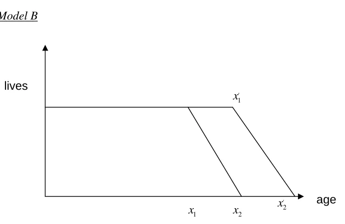
[image:20.595.93.441.109.335.2]Model B
Figure 5: Change in survival under model B
This time we have the difficulty of whether x1′ is greater or less than x2 i.e. how large the shift is.
Case (a) x1′ <x2
For t≤x1 i.e. before these new ‘healthier’ lives reach x1and don’t die.
Death rate
(
) (
)
2 1
2 1
x
x
l
x x l
x x
= − =
−
Which is the same as previously.
For x1< ≤t x1′ i.e. the new ‘healthier’ lives reach x1and don’t die but we still have some older lives dying.
Death rate
(
) (
) (
)
(
)
(
)
2 1 1 2
2 1 2 1 2 1
( )
x x x
l l l
x x t x x t
x x x x x x
= − − − = −
− − −
The first term is the same as above while the second term represents the lives that no longer die. As t increases this number increases which means that the total death rate decreases as t increases.
For x1′ < ≤t x2 i.e. the new ‘healthier’ lives reach x1′ and start to die at the new rate (which is actually the same as the old rate) and we still have some older lives dying.
1
x x2 x2′
1
x′ lives
However, the rate is changing as more of the new lives start getting exposed to ages they can die at.
Death rate
(
) (
) (
) (
)
(
(
)
)
2 1
2 1
2 1 2 1 2 1
x
x x l x x
l l
x t t x
x x x x x x
′ − ′
= − + − =
′ ′ ′ ′
− − −
The first term is the same as above (i.e. decreases as t increases as the old lives die out) while the second term are the new lives that are starting to die. As t increases this number increases. Note that for this period deaths are constant as the number of new lives dying is the same as the reduction in old lives dying (as the mortality rate for a given age where mortality occurs is not changed as the slope is identical).
For x2 < ≤t x2′ i.e. all the older lives have died off and the number of new lives dying is increasing as they start to reach the new maximum age.
Death rate
(
) (
)
1
2 1
x
l t x
x x
′ = −
′ − ′
As there are only new lives left we only have the new death rate but we haven’t reached the stable population yet. As t increases the number of people in the population and the number of deaths both increase.
For x2′ <t i.e. the new maximum age has been reached and the population is again stable
Death rate
(
) (
)
2 1
2 1
x
x
l
x x l
x x
′ ′
= − =
[image:21.595.72.438.445.703.2]′− ′
Figure 6: Deaths under model B
Note that the gradients are the same.
1
x x1′ x2′
2
x time
Case (b) x1′ <x2
For t≤x1 i.e. before the new ‘healthier’ lives reach x1
Death rate
(
) (
)
2 1
2 1
x
x
l
x x l
x x
= − =
−
Which is the usual death rate as seen in case a.
For x1< ≤t x2 i.e. the new ‘healthier’ lives reach x1and don’t die but we still have some older lives dying.
Death rate
(
) (
) (
)
(
)
(
)
2 1 1 2
2 1 2 1 2 1
( )
x x x
l l l
x x t x x t
x x x x x x
= − − − = −
− − −
This is the same death rate as in case (a) though the times when this process occurs differ.
Forx2 < ≤t x1′ i.e. the new lives haven’t reached x1′ so aren’t dying but all the old lives have died off => no one dies during this period!
Death rate = 0
For x1′< ≤t x2′ i.e. all the older lives have died off and the number of new lives dying is increasing as they pass the age where deaths start to occur, x1′, and start to reach the new maximum age x2′.
Death rate
(
) (
)
1
2 1
x
l t x
x x
′ = −
′ − ′
Again, we have seen this death rate in case (a) but with the time that this applies being different.
For x2′ <t i.e. the new maximum age has been reached and the population is again stable
Death rate
(
) (
)
2 1
2 1
x
x
l
x x l
x x
′ ′
= − =
Figure 7: Deaths under model B: alternative case ~ note that the gradients will be the same
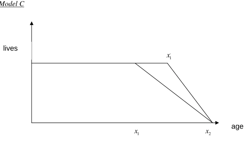
Model C
Figure 8: Effect of an increase in survival with no change in maximum age
For t≤x1 i.e. before these new ‘healthier’ lives reach x1
Death rate
(
) (
)
2 1
2 1
x
x
l
x x l
x x
= − =
−
Which is our usual result.
1
x x2
1
x′ lives
age
1 2 2
′
1
x
x x ′ x
deaths
[image:23.595.92.493.363.596.2]1 1
x < ≤t x′ i.e. the new ‘healthier’ lives reach x1 and don’t die but we still have some older lives dying
Death rate
(
) (
) (
)
(
)
(
)
2 1 1 2
2 1 2 1 2 1
( )
x x x
l l l
x x t x x t
x x x x x x
= − − − = −
− − −
This is the same as Model B.
Forx1′ < ≤t x2 i.e. the new ‘healthier’ lives reach x1′ and start to die at the new rate and we still have some older lives dying at the old rate.
Death rate
(
) (
) (
) (
)
2 1
2 1 2 1
x x
l l
x t t x
x x ′ x x
= − + −
′
− −
This is similar to Model 2 but the rates that the new and old population experience are different
For x2 <t i.e. the old lives die out and the population becomes stable once again
Death rate
(
) (
)
2 1
2 1
x
x
l
x x l
x x
′ ′
= − =
[image:24.595.96.500.364.640.2]′− ′
Figure 9: Transition in annual number of deaths over adjustment period
Generalised Model
We can see above that there are sections where two of the models experience similar rates to each other. In fact, what drives the three models are similar ideas i.e. how many ‘old’ and ‘new’ lives are dying at a given point in time. Allowing x1′ =x1 or
1
x x1′ x2
deaths
2 2
x′ =x then we can generalise the model initially into two parts; old lives and new lives.
Old lives
(
) (
)
(
) (
)
(
)
2 1 1
2 1
2 1 2
2 1
2 2 1
death rate =
0 0 x x x x l
x x l t x
x x
l
x t x t x
x x l x t x x ⎧ − = ≤ ⎪ − ⎪
⎪⎪ − < ≤
⎨ − ⎪ ⎪ = < ⎪ − ⎪⎩ New lives
(
)
(
) (
)
(
) (
)
1 2 11 1 2
2 1
2 1 2
2 1
0 0
death rate =
x x x x l t x x x l
t x x t x
x x
l
x x l x t
x x ⎧ ′ = ≤ ⎪ ′− ′ ⎪
⎪⎪ − ′ ′< ≤ ′
⎨ ′ − ′
⎪ ⎪
′ − ′ = ′ <
⎪
′ − ′ ⎪⎩
Of course, bringing the two equations together in this form brings problems with trying to set the boundaries. However, by using ‘Max’ and ‘Min’ functions we can combine both sets of equations into one equation.
( )
(
2 1 2)
(
)
(
( )
1 2 1)
(
)
2 1 2 1
death rate= , , lx , , lx
x Max Min t x x Min Max t x x x
x x ′ ′ ′ x x
− ⎡⎣ ⎤⎦ + ⎡⎣ ⎤⎦−
′ ′
− −
3. The empirical model
The theoretical model above allows many convenient results to be obtained. We now turn to the issues of whether such geometric shapes occur in reality by using the predictions and insights generated by the theory on real data. Our particular interests are ascertaining whether such patterns hold in reality and if they alter through time; if populations are converging to a maximum age with the passage of time; as life expectancy improves how many lives are saved year on year in different age bands, both in the past and future; and finally, using the model generated to forecast age-specific survival.
as far back as 1841. By studying these it is hoped that we can demonstrate that one of the three types of models detailed above can be used to model the results and forecasts we seek.
In the next section we illustrate aspects of continuous or broken evolution, convergence, divergence or parallelism from past data. In particular, results will be presented that show to what extent life is on track to converge to some upper limit and over what time period. This will be supported by a range of illustrative outputs including long-term projections of the annual number of avoided deaths at different ages based on trends in life expectancy and other potentially useful insights.
Data Sources
Life tables for England and Wales from 1841 to 2003 are contained in the Human Mortality Database (HMD, 2007), which has been available since 2000 and is the product of a joint collaboration between the Department of Demography at the University of California at Berkeley and the Max Plank Institute for Demographic Research. The HMD was created to provide detailed mortality and population data to researchers, and others interested in the history of human longevity. Its main goal is to document the longevity revolution of the modern era and to facilitate research into its causes and consequences (for more information, see www.mortality.org.)
The database contains original calculations of death rates and life tables for 33 national populations, as well as the raw data used in constructing those tables. A complete statement of the methodology used is contained in the methods protocol (Wilmoth et al, 2007). We illustrate examples of each predicted form of the survival curve using different starting ages and time windows. Our start ages are 1 year, 50 years and 80 years with a span of data running from 1841 to 2003, which are split into different time periods. Different time windows or starting ages produce distinctive patterns that are capable of particular interpretation and analysis going forward and backward in time.
Characterisation of changes based on life expectancy at age 1
(a) England and Wales (males)
[image:27.595.82.492.90.611.2](b) England and Wales (females)
Figure 10: Mortality percentiles as a function of life expectancy at 1, males (A) and females (B) from England and Wales
From the case with a starting age of 1 year in Figures 10 (a) and (b), it appears we can identify three eras as follows:
40 45 50 55 60 65 70 75 80 85
0 10 20 30 40 50 60 70 80 90 100 age at death
ex
pect
ed l
if
e
at
1
10th Percentile 20th Percentile 30th Percentile 40th Percentile 50th Percentile 60th Percentile 70th Percentile 80th Percentile 90th Percentile 1947
1901
A
B
C
1841 2003
40 45 50 55 60 65 70 75 80 85
0 10 20 30 40 50 60 70 80 90 100
Age at Death
E
x
pe
c
ted
l
if
e
at
1
10th Percentile 20th Percentile 30th Percentile 40th Percentile 50th Percentile 60th Percentile 70th Percentile 80th Percentile 90th Percentile 1901
1841 1947 2003
A – Starting in 1841 and ending in 1900 an era of rising life expectancy at age 1 from around 47 to 54 years (1.2 years per decade) for males and from 48 to 57 years for females (1.5 years per decade). During this era there was persistent high infant and childhood mortality, but reducing health inequalities at older ages as indicated by the convergence in the 20th to 90th mortality percentiles.
B - Starting in 1901 and ending in 1946, an era of rising life expectancy from around 54 to 67 years (2.8 years per decade) for males and from 57 years to 71 years (3.1 years per decade) for females. This more rapid improvement in life expectancy is mainly due to falling infant and childhood mortality and the continuing reduction in health inequalities as indicated by convergence in the 10th to 90th mortality percentiles.
C - Starting in 1947 to the present, an era of continuing rises in life expectancy from 67 to 76 years (1.6 years per decade) for males and from 71 years to 80 years (1.6 years per decade) for females. This slower improvement in life expectancy compared to B is due to the fact that childhood mortality had already been virtually eliminated at the start of this period so little improvement was achieved from reducing this further. Also the fall in convergence in other percentiles meant improvements in life expectancy was improved by a more parallel behaviour. The improvement in the lower percentiles was thus lower than before while the improvement at the higher percentile was greatest in this era.
We are able to split the results into 3 distinct eras because of more or less year on year improvements in life expectancy at this starting age. An exception is male years spanning the First World War, which interrupt the long run trend and have therefore been removed from Figure 10 (a). rather than starting at age 1, we could have used a start age of 0, but in this case we found that there was pattern loss due to high mortality at birth which tends to mask the underlying trend in the 10th percentile series in particular.
Starting age of 50
(a) England and Wales (males)
(B) England and Wales (females) G
(b) England and Wales (females)
Figure 11: Mortality percentiles as a function of life expectancy at 50, (a) males and (b) females England and Wales
Starting age of 80
Figures 12 (a) and (b), consider the pattern based on a starting age of 80 years. In this case it is evident that mortality percentiles acquire a divergent pattern indicating an increasing spread in the probability of death at older age coupled with rises in life expectancy. As in the previous case, up to 1901 the results show that improvements in life expectancy were uneven and that there were no net gains over the period with the pattern holding more or less constant whether life expectancy was increasing or decreasing. Post-1947 however, there has been more or less continuous improvement with life expectancy increases for males and females of between 2.3 and 2.6 years over the period.
15 17 19 21 23 25 27 29 31 33
50 55 60 65 70 75 80 85 90 95 100 Age at Death
E x pe c ted l if e at 50 10th Percentile 20th Percentile 30th Percentile 40th Percentile 50th Percentile 60th Percentile 70th Percentile 80th Percentile 90th Percentile 1947 1841 1901 1891 2003 15 17 19 21 23 25 27 29 31 33
50 55 60 65 70 75 80 85 90 95 100
Age at Death
(a) England and Wales (males)
(b) England and Wales (females)
Figure 12: Mortality percentiles as a function of life expectancy at 80, (a) males and (b) females England and Wales
Testing for convergence and maximum age
If these trends are to be used for forecasting future population survival an important question is how such patterns evolve, and whether a maximum age is indicated for example in convergent cases. However, as we have seen, continuation of such patterns is not necessarily guaranteed and if used to predict the future it is dependent on both the pace of progress in life expectancy and any changes in mortality patterns and the extent to which these can be anticipated.
0 1 2 3 4 5 6 7 8 9 10
80 81 82 83 84 85 86 87 88 89 90 91 92 93 94 95 96 97 98 99 100
Age at Death
E x pec ted l if e at 8 0 10th Percentile 20th Percentile 30th Percentile 40th Percentile 50th Percentile 60th Percentile 70th Percentile 80th Percentile 90th Percentile 1891 2003 1947 1901 1841 0 1 2 3 4 5 6 7 8 9 10
80 81 82 83 84 85 86 87 88 89 90 91 92 93 94 95 96 97 98 99 100
Age at Death
There would appear to be two main ways to project the data trends forward. The first is to project the percentiles forward using a basic relationship with the expected future lifetime as seen in the graphs above. A time frame can then be obtained by looking at how quickly expected future lifetime is increasing with respect to calendar year. The second method is to project the percentiles by comparing them directly to the calendar year.
To some extent this is a theoretical exercise as convergence fizzled out after 1946 but there is value in ascertaining what the maximum age would have been projected to be pre-1947, and how long it would have been expected to take to reach that point. The results can then be benchmarked against what has actually occurred
Consider the convergent pattern for females already indicated in section B of earlier Figure 10 covering the period 1901 to 1947. For the purposes of our analysis survival data for female lives for the year 1918 has been removed, as the influenza pandemic creates distortions in this year. It can be seen that the early deciles are converging towards the later ones though whether the later percentiles are converging or are parallel is harder to ascertain by sight.
To see whether convergence is occurring we fitted a linear regression to each decile. With these regressions we are able to determine which deciles are converging and also predict the expected life at age 1 required and the age of death where convergence would occur. The results are given below in Table 3 and presented in Figure 13.
Converging percentiles
Age of death where convergence
occurs
Required expected future lifetime at age 1
10th and 20th 83.91 83.16
20th and 30th 84.06 83.24
30th and 40th 86.14 84.96
40th and 50th 88.47 87.46
50th and 60th 92.28 92.58
60th and 70th 98.82 103.19
70th and 80th 102.89 110.86
80th and 90th 106.05 117.8
Table 3: Details of when deciles converge assuming linear regression
The above table can be easily interpreted when looking at one individual line. For example the top line states that the 10th and 20th percentiles will converge when the expected future lifetime at age 1 is 83.16 years and the age of death for these lives is 83.91.
However, there seems to be a problem when we look at the two columns together and it is easiest to illustrate with the last line. According to this line the 80th and 90th percentiles will converge when the expected future lifetime at age 1 is 117.8 but the age at death for these lives will be 106.05.
The problem is that the expected age at death is less than the expected future lifetime but these are the higher percentiles so the age of death should be higher than the expected future lifetime. This is seen in Figure 13 which is based on female data in the era from 1901 to 1947 and includes the fitted regressions lines projected to 1988.
As can be seen the inconsistency with expected future lifetime and age at death is that the graph inverts i.e. the 10th percentile would cross the 90th percentile before the 80th and 90th percentiles are anywhere near close. In fact the 80th and 90th percentiles cross when the expected future lifetime is 117.8 by which time the 10th percentile lives will be dying at age 178!
[image:32.595.86.482.402.607.2]There are a number of ways that we can get around this problem and most focus on looking at how the percentiles will behave once they have met. The first method that will lead to the quickest convergence is to consider that as the 10th percentile crosses the other percentiles it dominates and the improvement in mortality continues at the same pace that the 10th percentile has shown. In this case convergence will occur where the 10th and 90th percentiles converge. This takes place when the lives are expected to die at age 94.45.
Figure 13: Convergent case based on females from England and Wales, 1901 to 1946 with fitted regression lines
However, there is very little justification in the above assumption. As causes of death among the prematurely dying are a consequence of social, environmental or lifestyle changes it is hard to mount a case that improvements will continue at such a pace. Therefore when the 10th percentile meets the 20th percentile it is far more likely that the 20th percentile’s rate of mortality improvement carries on into the future. If this is the case then total convergence will only occur when the last percentiles meet, in this
50 55 60 65 70 75 80 85 90 95 100
0 10 20 30 40 50 60 70 80 90 100 age at death
expe
c
ted
l
if
e at
1
10th Percentile
20th Percentile
30th Percentile
40th Percentile
50th Percentile
60th Percentile
70th Percentile
80th Percentile
90th Percentile
case the 80th and 90th percentiles which will meet when the lives are expected to die at age 106.05.
Projecting time to convergence
While obtaining the ages of possible convergence is useful we also want to know if this will be in 10 years time or 1,000 years time. As we are basing the values of the percentiles on expected future lifetime we can analyse how fast this value is increasing and from this determine our convergence values.
For the years 1901-1951 a simple linear regression gives the equation
Expected future lifetime = calendar year * 0.3109 - 517.26
Under our first scenario we had the 10th and 90th percentiles converging when lives were expected to die at age 94.45. This equates to a nominal expected future lifetime of 87.038 (this is nominal as if we have convergence expected future lifetime would be 94.45-1 = 93.45). The value of 87.038 is obtained, assuming our regression is correct, in the calendar year 2001.65. In other words we should now have had convergence of mortality for females in the UK!
Under the second scenario we had the assumption that the slower improving percentile would dominate when percentiles meet. We can therefore reproduce table 3 from above and now calculate the year that these percentiles merge.
Converging percentiles
Age of death where convergence
occurs
Required expected future lifetime at age 1
Calendar Year this occurs
10th and 20th 83.91 83.16 1988
20th and 30th 84.06 83.24 1989
30th and 40th 86.14 84.96 1994
40th and 50th 88.47 87.46 2003
50th and 60th 92.28 92.58 2019
60th and 70th 98.82 103.19 2055
70th and 80th 102.89 110.86 2080
80th and 90th 106.05 117.8 2103
Table 4: Table showing age of death at convergence for different morality percentiles and the calendar year when this would be expected to occur
Converging percentiles
Calendar Year this occurs according to expected future
lifetime
Calendar year obtained projecting
lower percentile
Calendar year obtained projecting
upper percentile
10th and 20th 1988 1989 1988
20th and 30th 1989 1989 1989
30th and 40th 1994 1994 1995
40th and 50th 2003 2003 2003
50th and 60th 2019 2020 2021
60th and 70th 2055 2056 2058
70th and 80th 2080 2084 2087
[image:34.595.101.521.403.629.2]80th and 90th 2103 2111 2119
Table 5: Table showing the calendar year of convergence for different percentiles based on projecting the percentiles forward
Testing for parallelism
After 1951 the pattern changes from convergence to an apparently more parallel regime, at least visually, in which there is no convergence and therefore no upper age limit indicated. However, it is hard to find an occurrence of perfect parallel lines which last for any length of time. To illustrate this, below is a plot for male lives from 1952-2003 aged 50.
20 21 22 23 24 25 26 27 28 29 30
50 55 60 65 70 75 80 85 90 95 100
age at death
ex
pe
c
te
d
l
if
e
at
5
0
10th Percentile 20th Percentile 30th Percentile 40th Percentile 50th Percentile 60th Percentile 70th Percentile 80th Percentile 90th Percentile
Figure 14: Mortality percentiles for males from England Wales at age 50
Converging percentiles
Age of death where convergence
occurs
Required expected future lifetime at age
50
10th and 20th N/A N/A
20th and 30th N/A N/A
30th and 40th N/A N/A
40th and 50th 338.78 262.49
50th and 60th 287.95 216.61
60th and 70th 187.63 124.89
70th and 80th 139.26 79.53
80th and 90th 158.3 98.35
Table 6: Table showing age of death at convergence and expected future life time at age 50
This table is very different to the previous table. For the 10th, 20th and 30th percentiles we have divergence so we do not have values for convergence. Even the other percentiles which do converge do not do so for a number of years. For example, the first deciles to converge are predicted to be the 70th and 80th percentiles but this will only occur when the expected future lifetime of a 50 year old male is 79.53 years and these particular lives will live until they are 139.26 years old!
Testing for divergence
The divergence case appears to be restricted to the oldest starting ages. A convenient way to consider the pace of inter-decile divergence is either as a function of life expectancy, as in this illustration (Figure 15) at age 80, or a function of time.
Figure 15 shows that the inter-decile range (the gap in years between the 10th and 90th percentile) increases in direct proportion to life expectancy. For each one year increase in life expectancy, the female inter-decile range increases by 1.2 years (male by 1.5 years).
Note that there is a slight hint that the line may be non-linear, that the pace of divergence is slowing and that that divergence cannot proceed indefinitely in the current phase of human evolution.
The data points range from 1841 to 2003, but increases have not been continuous through time. As Figure 16 shows, until 1950 the inter-decile range for females fluctuated between 10 and 12 years, with minima occurring between 1880 and 1890. In this case the best fit curve is a second-degree polynomial (R2 = 0.91)