Nanoscale Resolution Interrogation Scheme
for Simultaneous Static and Dynamic
Fiber Bragg Grating Strain Sensing
Marcus Perry,
Student Member, IEEE,
Philip Orr,
Member, IEEE,
Pawel Niewczas,
Member, IEEE,
and
Michael Johnston
Abstract—A combined interrogation and signal processing technique which facilitates high-speed simultaneous static and dynamic strain demodulation of multiplexed fiber Bragg grating sensors is described. The scheme integrates passive, interferomet-ric wavelength-demodulation and fast optical switching between wavelength division multiplexer channels with signal extraction via a software lock-in amplifier and fast Fourier transform. Static and dynamic strain measurements with noise floors of 1nεand
∼10 nε/√Hz, between 5 mHz and 2 kHz were obtained. An inverse analysis applied to a cantilever beam set up was used to characterise and verify strain measurements using finite element modeling. By providing distributed measurements of both ulta-high-resolution static and dynamic strain, the proposed scheme will facilitate advanced structural health monitoring.
Index Terms—fiber Bragg gratings, optical fiber sensors, in-terrogation, structural health monitoring
I. INTRODUCTION
S
TRUCTURAL health monitoring of existing aging struc-tures and, particularly, future ‘smart’ strucstruc-tures will rely on advanced distributed measurements of not only high-frequency vibration, but also slowly changing strain [1]. Fiber Bragg gratings (FBGs) are often sought to meet these require-ments as they offer reliable, wavelength-encoded measure-ments of strain, that are immune to the interference and inten-sity fluctuations which plague conventional optical transducers [2]. However, when tasked with assessments of structural prestress loss or geological deformation, there are additional demands for stable, static strain sensors capable of nano-scale resolution. At the other extreme, vibration monitoring and impact detection may require highly responsive systems capable of surveying dynamic strain signals ranging from the seismic (1 mHz) to the ultrasonic (>20 kHz). Combining both static and dynamic monitoring capabilities into one demodulation unit will allow FBG monitoring solutions to remain cost-effective, while supplying a greater quantity of information to damage detection algorithms [3].Many contributions to the field of optical sensing have excelled in their respective static or dynamic fields indepen-dently. The application of cross-correlation algorithms to fiber
Manuscript received May 29, 2012; revised Aug 03, 2012. This work was supported by both EDF Energy and the Engineering and Physical Sciences Research Council.
M. Perry, P. Orr and P. Niewczas are with the Institute for Energy and Environment, University of Strathclyde, Glasgow, UK.(phone: +44(0) 141 548 4841; e-mail: [email protected].
M. Johnston is with EDF Energy Nuclear Generation Ltd, East Kilbride, UK.
Fabry-Perot sideband interrogation has yielded static strain resolutions as low as 0.8 nε [4]. Meanwhile, quasi-static and fully dynamic systems at 1.5 Hz and above 100 Hz have utilised frequency-locked lasers to provide noise spectral densities as low as 1.2 nε/√Hz and 0.3 pε/√Hz respec-tively [5], [6]. The schemes reported in the cited references, however, all suffer from resolution impairments after multi-plexing. For the static scheme, distributed sensing increases the already substantial measurement times (>10 s), while in the dynamic case, the requirement for a range of atomic-absorption lines makes multiplexing inconvenient. Bridging the gap between static and dynamic schemes while retaining full resolution, speed and multiplexing capabilities is therefore a key objective for optical structural health monitoring. While a small selection of schemes have been proposed to solve this problem [7], [8], there is still a growing and unmet demand for robust systems capable of combining distributed static and dynamic nanostrain-resolution measurements in a single interrogation unit. Such high-resolution systems would allow for the measurement of phenomena such as concrete creep and geodynamical changes in the earth’s crust [9], [10].
In this article, a passive, interferometric wavelength-demodulation technique [11] is combined with a fast optical path switch and a wavelength division multiplexing (WDM) module to provide an interrogation scheme which does not require tuning or modulation [12]. Signal extraction techniques such as a fast Fourier transform (FFT) and a software lock-in amplifier allow for high-speed, simultaneous, low-noise measurements of the static and oscillating strains in a mul-tiplexed FBG array. Measurements of the strain and natural frequency of a cantilever beam demonstrate the system’s ability to provide indicators of structural health using the inverse-method [13].
II. SYSTEMDESIGN
A. FBG Strain Sensor
Changes in strain,ε, and temperature,∆T, lead to fractional shifts in the reflected Bragg peak of an FBG given by [14]:
∆λB
λB
= (αΛ+αn)∆T+ (1−pe)ε (1)
phase difference:
φ=2πnsd
λ (2)
where ns and d are the refractive index and physical length difference of the two arms of the interferometer. Solutions to Maxwell’s equations state that the three outputs of the 3x3 coupler shown in Figure 1 must be mutually 120◦out of phase [16]. As such, the voltages at each photodetector (m= 1,2,3) at the MZI outputs, normalised to the first, can be described by:
¯
Vm=
Vm
C1
= Cm
C1
+Dm
C1
cos(φ+θm) (3)
where θm = 2π(m−1)/3 and Cm and Dm are constants which describe the amplitude of the dc and ac components of the interference fringes respectively. Crucially, the three outputs yield a phase measurement which is independent of any fluctuations in the optical intensity at the MZI input [17]:
tan(φ) = (µ2−µ3) ¯V1+ (µ3−µ1) ¯V2+ (µ1−µ2) ¯V3 (γ2−γ3) ¯V1+ (γ3−γ1) ¯V2+ (γ1−γ2) ¯V3
(4)
where µm = DCmmcos(θm) and γm = DCmmsin(θm) are re-trievable normalisation parameters, which depend on constants such as the mean intensity level, fringe visibility and optical losses within the setup. The photodetector voltages thereby provide a passive, robust and instantaneous demodulation of wavelength in one voltage sample, without the need for active modulation.
As the optical switch selects between the two FBGs, a square-wave of amplitude ∆φ= φref −φsens is generated. Differentiation of (2) with respect to wavelength and substitu-tion of (1) provides the conversion factor between FBG strain and measured phase differences:
∆ε= λ
2πnsd(1−pe)
∆φ (5)
The differential strain is then extracted from the square-wave by focusing on the component at the switching frequencyωs= 2πfs.
switching-frequencies can be retained and analysed. However, when seeking to extract only static strain, a software lock-in amplifier can provide a superior methodology [19]. In this case, the phase-locked sinusoidal reference signal used to drive the optical switch, g[n] = sin[ωrn], is multiplied with the signal square-wave to generate sum and difference frequency components. Sum frequency components are then rejected by a low-pass filter,G, leaving:
G(g[n].x[n]) =
2∆ε π
2N−1
X
l=1
cos[(jωs−ωr)nτ]
l (7)
wherel= 2k−1. When the reference and signal frequencies are equal (ωr = ωs), the first harmonic of the square-wave provides a dc voltage which is proportional to ∆ε. Noise is reduced, as only noise components close to the reference or signal frequencies are allowed to pass through the filter unat-tenuated. Conventionally, lock-in amplifiers are used in this manner to extract weak signals from a dominant background noise, but even low-noise systems can take full-advantage of the benefits, provided they are driven by a reference [20].
III. CHARACTERISATION
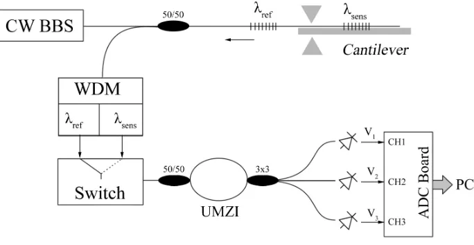
This section outlines the characterisation of the interrogation scheme for both static and dynamic strain measurements, which utilise the lock-in amplifier and FFT algorithms respec-tively. The experiment was set up as shown in Figure 1. One FBG atλsens=1554.66 nm was affixed to a cantilever using an epoxy adhesive, while another reference FBG in the vicinity is multiplexed atλref =1536.02 nm. The photodetectors were oversampled at a rate of fsp= 50 kHz, as this reduced the aliasing of higher harmonic components and improved FFT resolution. The optical switch selected at a rate fs= 500 Hz, while groups of N= 100 unfiltered data points were passed to a computer for signal extraction. A National Instruments software lock-in amplifier was filtered by a high-order Infinite Impulse Response (IIR) Chebyshev filter paramaterised by a cut-off frequency and roll-off of fF= 500 Hz and R= 200 dB/dec respectively.
Fig. 1. A continuous-wave broadband light source (CW BBS) illuminates a strain-sensing FBG,λsens, attached to a cantilever and an unstrained reference grating atλref. The WDM-switch set up allows for independent demodulation of the Bragg peaks by an unbalanced Mach-Zehnder interferometer (UMZI). Analogue-to-digital converted (ADC) voltage signals from the photodetectors are passed to a PC for further analysis.
period, a number, Γ, of strain differential measurements, were extracted from x[n]using the primary FFT and lock-in amplifier algorithms discussed in section II-C. A minimalist ‘max-min’ algorithm was also used to find the peak-to-peak amplitude of the square-wave by calculating the difference between its highest and lowest values. This algorithm worked by simply finding the magnitude of the samples which deviated furthest from the mean value in each half-cycle of ωs. The max-min algorithm resulted in a minimal response time, at the expense of higher noise and inaccuracy.
The standard deviation of a histogram of Γ = 1000 static strain measurements was used to gauge the resolution of the system for each algorithm. Temporal response was measured by striking the cantilever to generate a strain impulse. The tem-poral evolution of the lock-in and primary FFT were compared with the max-min method to provide an indication of relative time responses. A Fourier analysis of the strain differential was obtained using a secondary FFT ofΓ =400 strain differential measurements. This provided an assessment of the frequencies and magnitudes of dynamic strain components.
A. Cut-off Frequency
The lock-in amplifier’s static strain noise as a function of filter cut-off frequency is shown in Figure 3a). The excess sum and difference frequencies which result from signal-reference multiplication are gradually attenuated as the cut-off frequency is decreased from 10 kHz. Shown in Figure 3b) are the cut-off frequencies below 3 kHz. As shown strain noise eventually reaches a minimum of±1 nε. At this point, noise is no longer Gaussian and arises due to imperfect temperature compensation between the FBGs. Instabilities in the MZI are not to blame as the voltage outputs are affected proportionally by any changes in pathlength.
Note that as the filter settling time is inversely proportional to cut-off frequency, there is a trade-off between system response time and precision. Reducing the strain noise from 20 to 2nε can increase response times from 1 ms to 0.1 s.
Fig. 2. Block diagram outlining the steps used to assess relative algorithm performance. The voltages output from the interrogation scheme from the MZI and PDs (photodetectors) in Figure 1 are converted to a signal square-wave,
[image:3.612.338.536.313.642.2]Fig. 3. Strain noise,εrmsas a function of lock-in filter cut-off frequency,
fF between a) 10 Hz and 10kHz and b) 10 Hz and 3000 Hz. The turning point at around 5 kHz is due to the gradual rejection of the sum and difference frequencies arising from signal-reference multiplication. The current system is limited to a minimum noise of ±1 nε due to imperfect temperature compensation.R2values show the correlation coefficients of the fits.
B. Sample Size
Increasing the number of samples, N, passed to the FFT reduces the bin size, improving strain resolution at the expense of sensor response time. As shown in Figure 4, a minimum strain resolution of 5 nε was obtained for a 40 ms sampling time. Increasing N can thus make it challenging to resolve rapid, sequential impulses in the system. This problem equally affects the lock-in amplifier, which does not benefit from the increased sample sizes.
C. Switching Frequency
As shown in Figure 5, increasing the optical switching frequency dramatically improves the strain resolution of the lock-in amplifier, without reducing system response times. The reason stems from equation 7. The difference between the reference frequency and harmonics of the signal wave (lωs−ωr) takes larger values for higher switching rates. This reduces the likelihood of these components (and their aliases) from passing through the low-pass filter. The amplitude noise
[image:4.612.320.556.51.252.2]Fig. 4. Noise,εrms, in the strain measured by the FFT as a function of time lag,tL. These results were obtained by varying sample sizes in the rangeN=[100,1000]. The inverse square root dependence stems from the strain scaling with the square root of FFT power, and fits with a correlation factor of 0.9978.
Fig. 5. The dependence of FFT and lock-in strain noise,εrms, on the switching frequency, fS, for a cut-off frequency of 1 kHz. There is no correlation between switching frequency and amplitude noise in the FFT. In the lock-in amplifier, the linear introduction of harmonic power noise for reduced switching frequencies leads to an inverse square-root dependence between amplitude noise and switching rate (correlation coefficient 0.9949).
in the FFT, on the other hand, is independent of the switching rate, as it instead depends mainly on the rate and volume of sample acquisition.
D. High Frequency Measurements
[image:4.612.319.542.324.512.2]Fig. 6. Collection of secondary FFTs of FBG strain, as measured for a cantilever driven by a loudspeaker, operating at driving frequencies between 0.05 and 2 kHz. Variations in amplitude and secondary harmonics arise from resonant frequencies within the experimental set. Above 5 Hz, the noise floor is 7nε/√Hz.
A collection of secondary FFT spectra for various cantilever driving frequencies are shown in Figure 6. As shown, the system is fully capable of measuring sub-microstrain signals up to 2 kHz, with a noise floor of 7nε/√Hzabove 5 Hz.
Due to the two-step process, the second FFT’s frequency bandwidth is inversely proportional to the frequency bin size of the primary FFT. As the primary FFT must resolve the signal square-wave accurately, system bandwidth is, for the time being, limited by the 40 kHz sampling rate.
E. Low Frequency Measurements
The scheme’s ability to perform at seismic frequencies is demonstrated by increasing FFT sample sizes. This yields high frequency-resolution measurements of low (1 Hz) bandwidth strain oscillations. Driving the electroacoustic transducer at 80 mHz in both pulsed and sinusoidal modes results in the strain profiles and secondary FFTs shown in Figure 7. After a 200 s sampling time, the first few harmonics of both low-frequency signals were detected with a resolution of 5 mHz. Crucially for geophysical measurements, nanostrain resolutions have been retained, as the noise floor is 17nε/√Hzabove 50 mHz.
IV. APPLICATION TOSTATIC-DYNAMICSTRAIN
MEASUREMENT
Both the strain and natural frequency of a cantilever vary as a function of the force applied to the cantilever end. By finding the natural vibration frequencies and strains in the region that the FBG is bonded to, model values can be used to verify those obtained experimentally. Conventionally, the Euler-Bernoulli equation and the equation of motion for a fixed-free cantilever of thickness h, length L and mass Mb can be solved to find the longitudinal strain along the cantilever’s length, ε(z)and the natural angular frequency,ωC, for a given tip force,F:
ε(z) = (L−z)F h
2IE , ω
2
C=
3EI L3(0.2357M
[image:5.612.52.309.55.225.2]b+Fg) (8)
Fig. 7. Two low-frequency strain profiles and their resulting FFT spectra. a) shows the measured 0.08 Hz strain profiles applied to the cantilever over time for pulsed and sinusoidal actuation of the transducer. Performing primary and secondary FFTs over 4000 and 2000 samples respectively yield b). The FFT bandwidth extends to 1 Hz, but has been terminated earlier for clarity. The low bandwidth reduces the temporal response of the system to 200 s, but also provides a minimum measurable frequency 5 mHz. The noise floor above 50 mHz is 17nε/√Hz.
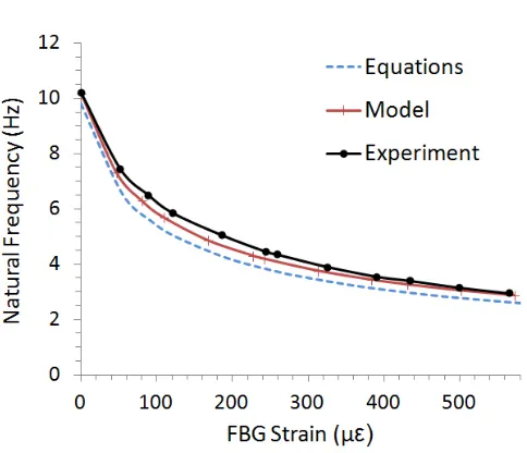
where E is the elastic moudulus, I is the second moment of area andg is gravitional acceleration. Significant improve-ments to accuracy, however, can be made through Finite Element Modelling (FEM) using COMSOL. The geometry, mesh and an example longitudinal strain for a realistic steel cantilever are shown in Figure 8. Structural mechanics and shell models were solved in stationary and eigenfrequency domains to find the static strain and natural frequencies of a cantilever, as a function of tip force.
inverse-Fig. 8. Original mesh and deformation of the cantilever beam under a tip force of 3.94N. The longitudinal strain is shown along the top surface of the cantilever.
Fig. 9. The natural frequency of the cantilever as a function of the strain measured by an FBG. Shown are the theoretical, finite element model (FEM) and measured values. Using a Young’s modulus of E=200 GPa allows excellent agreement between the modeled and measured values.
Slow drifts in the measured strain are thought to result from the fact that the reference and sensing FBGs have poor thermal contact. Indeed, there is only so much an interrogation scheme can do to reduce the noise before physical phenomena, such as these, must be rectified. Measurements in structural health monitoring depend equally on long-term, reliable mechanical and thermal contact between the sensors and the structure.
When choosing to extract signals through an FFT, the sample acquisition rates and volumes are of prime importance for a low strain noise. However, as increasing the number of samples also reduces the time resolution of the system, it is recommended that sampling rates are maximised as a first resort. Likewise, reductions in dc fluctuations in the lock-in amplifier can be achieved by increasing the switching frequency, but both of these hardware improvements may reduce the cost-effectiveness of the system.
Spectral leakage and aliasing currently cause negligible offsets in strain accuracy because samples are obtained in a frequent, well-defined, periodic manner. As such, there is no call for the implementation of window functions or pre-sample filtering to the signal sqauare-wave, both of which can be detrimental to system response and noise.
One criticism of this system is its inability to demodulate absolute wavelengths. The phase-unwrapping method only allows for relative strains to be monitored while the system is running, thus an extra interrogation device may be required if absolute strain cannot be inferred. It is worth noting, however, that many applications in structural health monitoring, such as measurements of prestress loss or geophysical deforma-tion, only induce or require the assessment of relative strain changes. The system’s dynamic range depends on the number of multiplexed FBGs in the sensor array and the channel widths and spacings of the CWDM, as FBG shifts must be prevented from overlapping between channels.
[image:6.612.54.296.461.669.2]multiplexing can be conveniently realised through the use of high (1 MHz) bandwidth or cascaded switches.
VI. CONCLUSION
The characteristics of a fiber Bragg grating interrogation scheme based on a three-output interferometer and a wave-length division multiplexing switching system were investi-gated. Using the proposed scheme, we have demonstrated the simultaneous interrogation of static and dynamic fiber Bragg grating nanostrain sensors. A software lock-in amplifier was used to extract static strain signals with a 1 nε resolution, which was limited by thermal fluctuations between FBGs. Various fast Fourier transform algorithms were applied to retrieve dynamic strain measurements in both seismic and audible frequency regimes. Frequency resolutions of 5 mHz and 5 Hz were obtained for bandwidths of 1 Hz and 2 kHz. In both cases, a high strain-resolution was retained as noise floors were 7 and 17 nε/√Hzrespectively.
Assessments of fixed and oscillating strains were employed to provide evaluations of the elasticity of a cantilever beam based on its natural frequency. These agreed with modeled and theoretical values. Further application of the model allowed for a full mechanical description of the cantilever, based on an inverse analysis. The scheme’s ability to scale conveniently to allow quasi-distributed strain measurements without resolution or response losses make it ideally suited to strain-based structural health monitoring applications, which will benefit from the dual-regime and distributed measurement attributes.
REFERENCES
[1] J. M. L´opez-Higuera, L. R. Cobo, A. Q. Incera, and A. Cobo, “Fiber optic sensors in structural health monitoring,” J. Lightwave Technol., vol. 29, pp. 587–608, Feb 2011.
[2] A. Kersey, M. Davis, H. Patrick, M. LeBlanc, K. Koo, C. Askins, M. Put-nam, and E. Friebele, “Fiber grating sensors,”Lightwave Technology, Journal of, vol. 15, pp. 1442–1463, Aug. 1997.
[3] N. Serker and Z. Wu, “Structural health monitoring using static and dynamic strain data from long-gage distributed FBG sensor,” IABSE-JSCE Joint Conference on Advances in Bridge Engineering-II, pp. 519– 526, 2010.
[4] Q. Liu, T. Tokunaga, and Z. He, “Sub-nano resolution fiber-optic static strain sensor using a sideband interrogation technique,” Opt. Lett., vol. 37, pp. 434–436, Feb 2012.
[5] A. Arie, B. Lissak, and M. Tur, “Static Fiber-Bragg Grating Strain Sensing Using Frequency-Locked Lasers,”J. Lighwave Tech., vol. 17, no. 10, pp. 1849–1855, 1999.
[6] J. H. Chow, D. E. McClelland, M. B. Gray, and I. C. M. Littler, “Demonstration of a passive subpicostrain fiber strain sensor,”Opt. Lett., vol. 30, pp. 1923–1925, Aug 2005.
[7] Y. Wang, Y. Cui, and B. Yun, “A Fiber Bragg Grating Sensor System for Simultaneously Static and Dynamic Measurements With a Wavelength-Swept Fiber Laser,”IEEE Phot. Tech. Lett., vol. 18, no. 14, 2006. [8] P. Antunes, H. Lima, H. Varum, and P. Andre, “Optical fiber sensors for
static and dynamic health monitoring of civil engineering infrastructures: Abode wall case study,”Measurement, vol. 45, no. 7, pp. 1695 – 1705, 2012.
[9] Z. Bazant, “Prediction of concrete creep and shrinkage: past, present and future,”Nucl. Eng. Des, vol. 203, no. 1, pp. 27 – 38, 2001. [10] P. Ferraro and G. D. Natale, “On the possible use of optical fiber bragg
gratings as strain sensors for geodynamical monitoring,” Opt. Laser. Eng., vol. 37, no. 23, pp. 115 – 130, 2002.
[11] M. Todd, G. Johnson, and C. Chang, “Passive, light intensity-independent interferometric method for fibre Bragg grating interroga-tion,”Elec. Lett., vol. 35, no. 22, pp. 784–786, 1999.
[12] P. Orr and P. Niewczas, “High-speed, solid state, interferometric inter-rogator and multiplexer for fibre bragg grating sensors,”J. Lightwave Techn, no. 99, pp. 1 – 1, 2011.
[13] M. I. Friswell, “Damage identification using inverse methods,”Royal So-ciety of London Philosophical Transactions Series A, vol. 365, pp. 393– 410, Feb. 2007.
[14] A. Othonos,Fiber Bragg gratings : fundamentals and applications in telecommunications and sensing. Boston Mass.: Artech House, 1999. [15] Y. Rao, “In-fibre bragg grating sensors,”Meas. Sci. and Tech., vol. 8,
no. 4, p. 355, 1997.
[16] P. E. Greene, Fiber Optic Networks. New Jersey: Prentice Hall, 1993. [17] M. Todd, M. Seaver, and F. Bucholtz, “Improved, operationally passive interferometric demodulation method using 3x3 coupler,” Elec. Lett., vol. 38, no. 15, pp. 784–786, 2002.
[18] M. Boas, Mathematical Methods in the Physical Sciences. New Jersey: Wiley, 3rd ed., 2005.
[19] J. Scofield, “A Frequency-Domain Description of a Lock-in Amplifier,”
Amer. J. Phys, vol. 62, no. 2, pp. 129–133, 1994.
[20] R. Burdett, Amplitude Modulated Signals: The Lock-in Amplifier. New Jersey: Wiley, 2005.
Marcus Perry received an MSci degree in Physics from the University of Bristol, UK in 2009. He is currently working with EDF Energy towards an Engineering Doctorate in optical fiber sensors for use in nuclear environments at the Institute for Energy and Environment, University of Strathclyde. His research focuses on the use of fiber Bragg grating strain sensors for monitoring prestress loss in fission reactor prestressed concrete pressure vessels.
Philip Orrreceived the BEng and PhD degrees in electronic and electrical engineering in 2007 and 2011 respectively from the University of Strathclyde, where he is presently a research associate with the Institute for Energy and Environment. His core research area is the fundamental design of fibre sensors and interrogators for application within power and energy systems. In particular, he is concerned with intrinsic fibre sensing, multiplexing topologies, electromagnetic field measurement, nuclear diagnostics, and power system protection.
Pawel Niewczas received his PhD in the area of optical current sensors from the University of Strathclyde in 2000. He is currently a Senior Lecturer in the Department of Electronic and Electrical Engineering, University of Strathclyde, and is leading the Advanced Sensors Team within the Institute for Energy and Environment in the same department. His main interests centre on the advancement of optical sensing methods in such areas as power system metering and protection; gas turbine monitoring; downhole pressure, temperature, voltage and current measurement and in nuclear fission and fusion environments. He has published over 60 technical papers in this area.
![Fig. 4.Noise, εrms, in the strain measured by the FFT as a function oftime lag, tL. These results were obtained by varying sample sizes in therange N=[100,1000]](https://thumb-us.123doks.com/thumbv2/123dok_us/1677849.121223/4.612.54.295.50.419/strain-measured-function-oftime-results-obtained-varying-therange.webp)