TERMINAL MULTIPLE SURFACE SLIDING GUIDANCE FOR
PLANETARY LANDING: DEVELOPMENT, TUNING AND
OPTIMIZATION VIA REINFORCEMENT LEARNING
Roberto Furfaro
*, Daniel R. Wibben,
†Brian Gaudet
‡, Jules Simo
§The problem of achieving pinpoint landing accuracy in future space missions to planetary bodies such as the Moon or Mars presents many challenges, including the requirements of higher accuracy and degree of flexibility. These new challenges may require the development of a new class of guidance algorithms. In this paper, a non-linear guidance algorithm for planetary landing is proposed and analyzed. Based on Higher-Order Sliding Control (HOSC) theory, the Multiple Sliding Surface Guidance (MSSG) algorithm has been specifically designed to take advantage of the ability of the system to reach multiple sliding surfaces in a finite time. As a result, a guidance law that is both globally stable and robust against unknown, but bounded perturbations is devised. The proposed MSSG does not require any off-line trajectory generation, but the acceleration command is instead generated directly as function of the current and final (target) state. However, after initial analysis, it has been noted that the performance of MSSG critically depends on the choice in guidance gains. MSSG-guided trajectories have been compared to an open-loop fuel-efficient solution to investigate the relationship between the MSSG fuel performance and the selection of the guidance parameters. A full study has been executed to investigate and tune the parameters of MSSG utilizing reinforcement learning in order to truly optimize the performance of the MSSG algorithm in powered descent scenarios. Results show that the MSSG algorithm can indeed generate closed-loop trajectories that come very close to the optimal solution in terms of fuel usage. A full comparison of the trajectories is included, as well as a further Monte Carlo analysis examining the guidance errors of the MSSG algorithm under perturbed conditions using the optimized set of parameters.
INTRODUCTION
Future planetary missions, both robotic and human, will require unprecedented levels of landing accuracy and system flexibility. As an example, over the past decade, landing systems developed for Mars missions have been critical to ensure the successful deployment of agents (e.g. rovers, landers) on the Martian surface and it will continue to grow in importance due to the sustained interest of the scientific community to explore the red planet [1],[2]. In addition, there has been recent renewed interest in the Moon and its potential economic returns by mining for the various resources that it contains[3]. In both cases, more demanding planetary exploration requirements translate to technology development that calls for more precise guidance systems capable of delivering rovers and/or landers with higher degree of precision. In past missions to both the Moon and Mars, delivery of robotic agents to the ground was ensured with a safe landing
*
Assistant Professor, Department of Systems and Industrial Engineering, Department of Aerospace and Mechanical Engineering, University of Arizona, 1127 E. James E. Roger Way, Tucson, Arizona, 85721, USA
†
Graduate Student, Department of Systems and Industrial Engineering, University of Arizona, 1127 E. James E. Roger Way, Tucson, Arizona, 85721, USA
‡
Research Engineer, Department of Systems and Industrial Engineering, University of Arizona, 1127 E. James E. Roger Way, Tucson, Arizona, 85721, USA
§
without the need of higher precision. In the case of Mars, the landing accuracy, usually described by a 3-sigma landing ellipse, has been established to be on the order of 100 km (e.g. Phoenix Mission, MER). The recent landing of the Mars Science Laboratory (MSL) has taken important steps towards increasing the precision of landing on Mars. Indeed, the MSL system architecture included an Apollo-derived guidance algorithm employing bank angle control during the initial atmospheric entry as well as a powered descent algorithm designed to deliver to the surface the newly designed “Sky Crane” system within 10 km accuracy [4]. Despite these improvements, future missions may require an even higher landing precision to possibly pinpoint level (10s of meters).
Powered descent algorithms generally comprise of two major components: a) a targeting (trajectory planning) algorithm and b) a trajectory-following, real-time guidance algorithm. The targeting algorithm is responsible for generating a reference trajectory (position, velocity, and thrust profile) that explicitly defines the path for driving the vehicle to the desired landing location. Subsequently, the trajectory-tracking algorithm is designed to close the loop on the desired trajectory ensuring that the spacecraft follows the planned path. Current practice for Mars landing employs a guidance approach where the reference trajectory is generated on-board5. More specifically, the trajectory is computed as a fifth-order polynomial whose coefficients are determined by solving a Two-Point Boundary Value Problem (TPBVP). Originally devised to compute the reference trajectory used by the Lunar Exploration Module [6]-[8], the method is currently employed to generate a feasible reference trajectory comprising of the three segments of the MSL powered descent phase5. A fifth-order (minimal) polynomial in time satisfies the boundary condition for each of the three position components. The required coefficients can be determined analytically as a function of the pre-determined time-to-go.
Recently, more research efforts have been devoted towards determining reference trajectories (and guidance commands) that are fuel-optimal, i.e. trajectories that satisfy both the desired boundary conditions and any additional constraints while minimizing the fuel usage [9]-[11]. Whereas analytical solutions are possible for a limited number of cases (e.g. the energy-optimal landing problem with constant gravity and unconstrained thrust [12]), fuel-efficient trajectories can be found numerically using either direct or indirect methods. Solutions based on direct methods are generally obtained by converting the infinite-dimensional optimal control problem into a finite constrained Non-Linear Programming (NLP) problem [13]. Recently, Acikmese et al.[11] devised a convex optimization approach where the minimum-fuel soft landing problem is cast as a Second Order Cone Programming problem (SOCP)[14]. The authors showed that the appropriate choice of a slack variable can convexify the problem [15]. Consequently, the resulting optimal problem can be solved in polynomial time using interior-point method algorithms [16]. In such a case and for a prescribed accuracy, convergence is guaranteed to the global minimum within a finite number of iterations. The latter makes the method attractive for possible future on-board implementation. Moreover, the method has been extended to find solutions where optimal trajectories to the target do not exist, i.e. the guidance algorithm finds trajectories that are safe and closest to the desired target [17].
algorithms for endo-atmospheric flight system guidance (e.g. missiles [23]). In particular, sliding control methods have emerged as attractive techniques that can be applied to develop robust missile autopilots [24],[25] and guidance algorithms [26],[27]. However, such non-linear guidance design methods have rarely been used to design guidance algorithms for planetary precision landing. Recently, Furfaro et al. have explored sliding control theory as a mean to develop two classes of robust guidance algorithms for precision lunar landing [28]. In addition, the potential use of HOSC for asteroid close proximity-operation has been studied [30]. In the context of autonomous guidance for missions to small bodies, Furfaro et al. [29] developed a Multiple Surface Sliding Guidance (MSSG) algorithm for asteroid precision landing. The MSSG approach results in a guidance algorithm that is robust against perturbations and unmodeled dynamics. MSSG, which is designed on the principles of 2-sliding mode control, employs multiple sliding surfaces to generate on-line targeting trajectories that are guaranteed to be globally stable under bounded perturbations (with known upper bound [18],[21]). Two sliding surface vectors are concatenated in such a way that an acceleration command program that drives the second surface to zero automatically drives the dynamical system on the first surface in a finite time. The on-line trajectory generation and the determination of the guidance command require only knowledge of the system state (position and velocity) and the desired landing position. Importantly, one of the key principles behind the proposed methodology is that the landing problem is considered complete once the sliding surface is reached, i.e. the dynamical system reaches the surface for the first time at the landing location (with the desired velocity). Such approach has been first proposed and discussed by Harl and Balakrishnan who applied HOSC to design a class of sliding-based guidance algorithms for the terminal guidance of an unpowered lifting vehicle during the approach and landing phase [31].
In this paper we demonstrate that the MSSG algorithm can be potentially employed as terminal guidance for general planetary pin-point landing, i.e. it is possible to generate closed-loop landing trajectories on large planetary bodies that are precise and robust against perturbations and un-modeled dynamics. Importantly, while the proposed algorithm has been shown to be robust and globally stable in the previous work done by Furfaro et al. [28]-[30], preliminary results have demonstrated that it is sensitive to the guidance parameters and it is generally sub-optimal for any given set of parameters. Whereas the latter may not be a limiting factor for small body guidance, fuel-efficiency becomes critical for landing on planets and moons. This paper aims at investigating the general behavior of the MSSG guidance for planetary bodies as well as employing Reinforcement Learning (RL [32]) to select (learn) the set of guidance gains that optimize MSSG in terms of both residual guidance error and fuel usage. Within the RL framework, the guidance problem is cast as a Markov Decision Problem (MDP) which enables the determination of a set of guidance parameters that are optimized in a stochastic environment. The goal is to demonstrate that RL can be effectively used to tune the MSSG algorithm to maximize performance in terms of landing error and fuel consumption while preserving the intrinsic characteristic of stability and robustness.
TERMINAL GUIDANCE PROBLEM FORMULATION
We consider the terminal planetary descent and landing guidance problem that can be formulated as follows: given the current state of the spacecraft, determine a real-time acceleration program that reaches the target point on the surface with zero velocity.
Dynamical Model: 3-D Equations of Motion
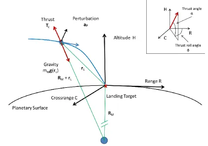
The fundamental equations of motion of a spacecraft moving in the gravitational field of a planetary body can be described using Newton’s law (Figure 1). Assuming a mass variant system, the equations of motion can be written as:
̇ (1)
̇
‖ ‖ ( ) (2)
̇
(3)
Here, and are the position and velocity of the lander with respect to a coordinate system with origin on the planet’s surface, is the gravitational constant of the moon, is the planet radius, is the thrust vector, is the mass of the spacecraft, is the specific impulse of the lander’s propulsion system, is the reference gravity, and is a vector that accounts for unmodeled forces (e.g. thrust misalignment, effect of higher order gravitational harmonics, atmospheric drag, etc.). If [ ] and [ ] the equations of motion can be written by components as:
̇ (4)
̇ (5)
̇ (6)
̇
‖ ‖
(7)
̇
‖ ‖
(8)
̇
‖ ‖
(9)
̇
(10)
The considered mathematical model is a 3-DOF model with variable mass. This model is employed to simulate spacecraft descent dynamics by the proposed guidance law.
Figure 1.Guidance Reference Frame and Free-Body Force Diagram for a Planetary Lander during the Powered Descent to the Designated Target
NON-LINEAR LANDING GUIDANCE LAW DEVELOPMENT
Sliding Control Theory for Systems of Higher Relative Degree
The sliding control methodology is an elementary approach to robust control [33]. Intuitively, it is based on the observation that it is much easier to control non-linear and uncertain 1st order systems (i.e. described by first-order differential equations) than nth-order systems (i.e. described by nth-order differential equations). Generally, if a transformation is found such that an nth-order problem can be replaced by a first-order problem, it can be shown that, for the transformed problem, perfect performance can be achieved in presence of uncertain modeled dynamics.
Consider the following single-input, nth-order dynamical system:
( ) ( ) (11)
assumed to be not exactly known. Under the conditions that both ( ) and ( ) have a known upper bound, the sliding control goal is to get the state to track the desired state
[ ̇ ( )] in presence of model uncertainties. The time varying sliding surface is introduced as a function of the tracking error ̃ by the following scalar equation:
( ) (
)
̃ (12)
For example, for the case , one obtains:
( ) ̃̇ ̃ (13)
Here, is a positive constant. According to Eq. (12) and Eq. (13), the tracking problem is reduced to the problem of forcing the dynamical system in Eq. (11) to remain on the time-varying sliding surface (Eq. (13)). Clearly, tracking an n-dimensional vector has been reduced to the problem of keeping the scalar sliding surface to zero. The system’s stabilization can be now achieved by selecting a control law such that outside the sliding surface the following is satisfied:
(14)
Here, η is a strictly positive constant. Eq. (14), also called “sliding condition”, explicitly states that the distance from the sliding surface decreases along all system trajectories. Generally, constructing a control law that satisfies the sliding condition is fairly straightforward. For example, using the Lyapunov direct method [34], one can select a candidate Lyapunov function as follows:
( ) (15)
where ( ) and ( ) for . By taking the derivative of Eq. (15), it is easily concluded that the sliding condition (Eq. (14)) is satisfied. The control law is generally obtained by substituting the sliding control definition, Eq. (13), and the system dynamical equations, Eq. (11), into Eq. (14).
Definition: Consider a smooth dynamical system with a smooth output ( ) (sliding function). Then, provided that ̇ ̈ are continuous and that ̇ ̈ , then the motion on the set { ̇ ̈ } { } is said to exist on a r-sliding mode.
As it will be shown shortly, the dynamics of the soft landing problem are such that the acceleration command appears in the second derivative of a properly defined sliding vector. Thus, 2-sliding control principles can be applied to take advantage of such properties and ameliorate/reduce the chattering by pushing it at higher order. Recently, HOSC has been one of the central topics of modern non-linear control theory [18]-[22]. Indeed, asymptotically stable higher-order sliding modes appear naturally in systems that are traditionally treated with conventional sliding-mode control [35]. Whereas theoretical studies on the finite-convergence properties of arbitrary-order sliding mode control are currently underway (e.g. Levant [20]), 2-sliding controllers have been already applied in practical problems of interest in space and aerospace applications including missile guidance [24]-[27], reentry terminal guidance [31] as well as lunar and asteroid landing guidance [28],[30]. Importantly, Harl and Balakrishnan [31] set the stage on how to apply HOSC principles for terminal landing guidance problems. The key point is to enforce that the sliding surface and its derivative will go to zero in a finite time while ensuring that both will not cross zero until the final time is achieved. In contrast with one of the most popular approaches described by Levant [21] where 2-sliding homogeneous control can “twist” around the sliding surface zeroing it out in a finite time, such approach is not suitable for guidance applications as the problem is considered over when the sliding surface is crossed (i.e. the lander has reached the desired target point). Notably, the idea of devising robust guidance algorithms such that the sliding surface is reached in finite time for the first time at the landing location can be also effectively employed in standard sliding mode control as demonstrated for lunar landing [28].
The proposed MSSG for terminal planetary pinpoint landing is designed around the principles of HOSC. The overall approach to the MSSG development is to employ the notion that the motion of the guided vehicle during the powered descent toward the planet surface is forced to exist in a 2-sliding mode. The guidance law is derived in the next section.
Multiple Sliding Surface Guidance Development: HOSC approach to the Design of Terminal Planetary Landing Guidance
The overall goal is to derive a guidance law (acceleration command) that is a) robust against unmodeled disturbances, b) does not require a reference trajectory and c) guarantees the high performance requested by stringent precision requirements (i.e. pinpoint landing). The guidance model employed to develop the MSSG algorithm is a 3-DOF model similar to the one presented in the previous section (see Eq. (1)). However, the guidance model does not account for mass variation. The equations can be synthetically represented as follows:
(16a)
( ) ( ) (16b)
interest to the planetary powered descent problem, the dynamics of the sliding system has relative degree 2. Let us define the first sliding vector surface in the following way:
(17)
Here, is the position of the desired (target) landing point on the planet’s surface. Taking the derivative of , one obtains:
̇ ̇ ̇ (18)
Here, is the desired landing velocity (i.e. zero for soft landing). The guidance problem can be set as a standard control problem where the acceleration (guidance) command must be found such that ̇ in a finite time . It is easily verified that the sliding surface is of relative degree 2:
̈ ̇ ( ) (19)
Here the controller appears in the second derivative of the sliding surface. The acceleration algorithm is constructed by setting ̇ as a virtual controller and employing a backstepping approach. More specifically, ̇ is found such that the first sliding surface is driven to zero in a finite time. The virtual controller can be conveniently selected as follows:
̇ ( ) (20)
where, { } is a diagonal matrix of guidance gains. It is easily shown that the virtual controller ̇ is a) globally stable and b) it is able to drive the first sliding surface to zero in a finite time. Indeed, consider the following candidate Lyapunov function:
(21)
has the following properties:
( ) (22a)
( ) (22b)
The time-derivative of is negative definite everywhere:
̇ ̇ ( ) (
)( ) (23)
Here, { } are the cartesian components of the first sliding surface vector. Eq. (23) holds if { } . Generally, it is desirable that the matrix gains are all greater than one. Indeed, this can be seen in the time variation of the sliding surface vector , which can be explicitly derived. Applying separation to Eq. (20), one obtains:
(24)
Eq. (24) can be integrated to obtain the following:
( ) ( ) (25)
By imposing the initial conditions ( ) and taking the exponential of both sides, the solution becomes:
( ) ( ) (26) Or in vector form:
( ) ( ) (27)
The derivative of the sliding surface vector can be also computed explicitly:
̇ ( ) ( ) (28)
Or in vector form
̇ ( ) ( ) (29)
( ), both the sliding surface vector and its derivative go to zero for (i.e. at the desired reaching time).
At the point where the power descent is initiated, the spacecraft is generally characterized by a position and velocity such that Eq. (20) is not satisfied. Importantly, ̇ must be explictly connected to the acceleration command that drives both and ̇ to zero. Consequently, a second surface can be defined such that the acceleration command drives ̇ from its initial value to a trajectory defined by the first-order non-linear equation Eq. (20) which must be maintained until
̇ . A second sliding surface vector is defined in the following way:
̇ ( ) (30)
Importantly, the new sliding surface vector is of relative degree 1 with respect to the acceleration command. It can be easily verified that the acceleration command appears explicitly on the first derivative of :
̇ ̈ (
) ̇ ( ) ( ) ( ) ̇ ( ) (31)
The acceleration command is determined via a Lyapunov approach. Let us define a second Lyapunov candidate function as follows:
(32)
satisfies conditions similar to the one defined for (see Eq. (22)). Moreover, its time derivative becomes:
̇ ̇ { ( ) ( ( ) ̇
) } (33)
The acceleration command can be selected as follows:
{ ( ) ( ( ) ̇ ) ( )} (34)
Here, the matrix coefficients { }are defined as follows:
( )
With the parameter established by Eq. (35), it is guaranteed that the second sliding surface vector is driven to zero in a finite time . In fact, using Eq. (34), the equation describing the dynamics of the second sliding surface vector (Eq. (31)) becomes:
̇ ( ) (36)
Noting that does not change sign before reaching zero, Eq. (36) can be integrated between zero and to yield:
( ) ( ) ( ) (37)
Clearly, the second sliding surface vector goes to zero as . The MSSG law can be shown to be globally stable. Eq. (33) can be recast to consider the perturbing acceleration as well as the derived guidance law:
̇ ̇ { ( ) ( )} (38)
Thus, the time derivative of the second Lyapunov function is always less than zero if an upper bound for the perturbing acceleration, , is available. In such a case, the matrix coefficients can be selected such that | |. The second Lyapunov function is therefore decrescent and by virtue of the Lyapunov theorem for finite-time stability of non-autonomous systems,
as . Consequently, ̇ as .
As pointed out by the Harl and Balakrishnan [31] the adaptive nature of the guidance law is such that the system cannot be maintained on the first sliding surface for (see Eq. (26-29)). However, for the soft landing guidance problem, the latter is a non-issue as the problem is over as soon as the system reaches the final time.
Markov Decision Process and Reinforcement Learning: Tuning the Guidance Parameters
Sometimes called approximate dynamic programming, Reinforcement Learning [32] is a machine learning technique concerned with how an agent (e.g. the lander) must take actions in uncertain environments to maximize a cumulative reward (e.g. minimize the landing errors, minimizing fuel consumption). The stochastic environment is conventionally formulated as a Markov Decision Process (MDP) where the transition between states for a given action is modeled using appropriate transition probability. A MDP consists of:
• A set of states (where denotes a state ) • A set of actions (where denotes an action )
• State transition probabilities, which defines the probability distribution over the new state
that will be transitioned to given action is taken while in state • An optional discount rate that is typically used for infinite horizon problems
RL algorithms can learn a policy ( ) that maps each state to an optimal action. For a given state, these actions are considered optimal if they maximize the policy’s utility over the resulting system’s trajectory. The utility is defined as the expected value of the sum of discounted rewards computed starting from state and following the policy . For a single trajectory i, one can write the following:
( )( ) [ ( ( )) ( ( )) ( ( ))
] (39)
Here, the expectation accounts for the stochastic nature of the environment, whereas the sequence ( ) ( ) ( ) defines the trajectory associated with starting from initial condition .
To conceptually illustrate how the RL theory can be applied to design adaptive controllers, consider the problem of stabilizing an inverted pendulum attached to a cart on a bounded track. From a control design point of view, for any possible starting location on the track, it is desired to generate an acceleration command that keeps the angle of the pendulum with the vertical axis within some specified target value. Any possible starting location will define a unique trajectory - possibly over an infinite horizon, unless the controller finds a steady state control that keeps the pendulum balanced. For the cart control problem and given the current system state, reinforcement learning means that a policy that will generate an optimal action (i.e. an acceleration along the track) is learned through real or simulated experience. The action will be determined to be optimal with respect to the problem’s definition of utility. For this type of problem, one can estimate a policy’s utility using a sampling approach. In such a case, the estimate would be calculated as either the average or minimum utility over the sample trajectories:
( ) ∑ ( )( )
( ) ( )( ) (40)
Note that the concepts used to define the reinforcement learning problem have a clear counterpart to those used to define the optimal control problem: the policy becomes the controller, the action becomes the control, the state transition probabilities becomes the plant, the utility becomes the negative cost, while the state remains the same.
Many RL-based algorithms approach the problem of determining the optimal policy indirectly, i.e. through the value function. For a given policy , the value function is defined as the expected sum of rewards given that the system is in state and executes policy . The value function can be expressed in terms of the reward associated with being in the current state plus the discounted expectation over the distribution of the next states given that the controller is following policy :
( ) ( ) ∑ ( )( ) ( )
determined by taking the action that maximizes the expected sum of future rewards for the given current state; using Equation (39), the optimally policy can be formally expressed as follows:
( )
∑ ( ) ( )
(42)
The principal limitation of this approach is that both the state and action space must be discretized. As a result, the number of discrete states and actions grow exponentially with the dimensionality of the state and action spaces. Often the state space has higher dimensionality than the action space; consequently it is often easier to discretize the action space than the state space. When this is the case, fitted value iteration, which learns a model that represents the value function as a continuous function of the state, may be effectively employed to determine the optimal policy. Suitable value approximation functions for fitted value iteration include least squares, weighted least squares, and neural networks using on-line learning. When it is desired to work with continuous state and action spaces, one approach (policy optimization) is to dispense with the value function, and directly search for the optimal policy.
The RL framework can be employed to optimize the MSSG guidance parameters. In this case, the RL theory is not directly applied to determine the optimal action as function of the state, but rather to determine (learn) the set of optimal guidance gains as function of the state (current or initial). Importantly, the landing problem is cast as MDP and the MSSG-guided descent is simulated in a stochastic environment where the guidance gains are iteratively updated to maximize a properly chosen reward function. Details of the optimization process are presented in the next sections.
RESULTS AND ANALYSIS
Initial Comparison to an Open-Loop Optimal Solution
As shown in Eq. (34), the guidance algorithms depends on five guidance parameters: , and ( ). The general behavior of the MSSG-generated trajectories can be assessed. The algorithm performance analysis is investigated in a powered lunar landing scenario. In order to investigate the effect of these parameters on the closed-loop trajectories, the MSSG guidance algorithm is compared from a fuel-usage standpoint to an open-loop, fuel-optimal lunar landing guidance solution found numerically via pseudo-spectral methods for the problem of lunar landing. The minimum-fuel optimal guidance problem can be formulated as follows [11]:
Minimum-Fuel Problem: Find the thrust program that minimizes the following cost function
(negative of the lander final mass; equivalent to minimizing the amount of propellant during descent):
̈ (44)
‖ ‖ (45) and the following boundary conditions and additional constraints: ‖ ‖ (46)
( ) ( ) ̇ ( ) (47)
( ) ( ) ̇ ( ) (48)
( ) (49)
Figure 2. Comparison of MSSG System Trajectories to Optimal Solution
The open-loop,fuel-optimal lunar landing problem is solved assuming that the lander’s initial position and velocity are ( ) [ ] and ( ) [ ] , respectively. Note that this initial state is similar to the apollo lander’s state at the beginning of the approach phase [8]. The guidance reference frame is fixed to the lunar surface with the origin located at the targeted landing point. The desired final state of the vehicle is set to be ( )
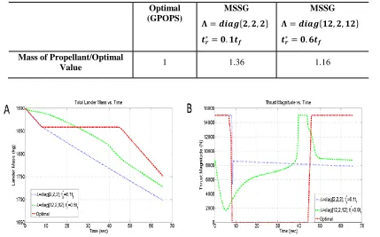
[ ] and ( ) [ ] . Targeting a point 10 meters above the lunar surface provides additional margin if any hazard avoidance maneuver is required.The lander is assumed to be a small robotic vehicle, with six throttlable engines ( ). For these simulations, the only dynamical force included is the gravitational force of the moon, as seen in Eq. (44). The lander is assumed to weigh 1900 kg (wet mass) and is capable of a maximum (allowable) thrust of 15 kN as well as a minimum (allowable) thrust of 1.5 N. While this lower thrust limit may not be truly realistic, it provides an extremely idealistic optimal case with which we can compare to the MSSG trajectories. The terminal position is set to be at the origin of the guidance reference frame to be achieved with zero velocity (soft landing). For comparison, the MSSG algorithm is initiated at the same initial conditions and defined to target the same terminal state. Figure 2 shows the trajectories and total velocity histories for the open-loop, fuel-optimal landing guidance found via GPOPS and two MSSG-guided cases. GPOPS found a total optimal flight time equal to
lower thrust limit imposed on the optimal solution, but instead feature a minimum thrust limit of approximately 3000 N. For the same descent time, the MSSG algorithm tends to require more fuel mass than the optimal case. The fuel-efficient thrust profile is extremal, i.e. the optimal algorithm thrusts at a maximum value until it switches to the minimum allowable thrust, and finally returns to the maximum value (bang-bang type). The MSSG algorithms reduce the thrust command until the second surface is reached. At , the thrust command experiences a large shift and then decreases monotonically until the first surface is achieved. The thrust spike can be in principle reduced by increasing . However, arbitrarly increasing (or decreasing) the time of flight can increase the fuel consumption [29].
Table 1. Comparison Between the Open-Loop Fuel-Optimal Guidance and the MSSG Guidance (Propellant Mass)
Optimal (GPOPS)
MSSG
{ }
MSSG
{ }
Mass of Propellant/Optimal
Value 1 1.36 1.16
Figure 3.A) Lander Mass and B) Thrust Magnitude Histories Comparing Optimal Solution to MSSG
Clearly, MSSG is sub-optimal. Indeed, in order to better characterize the performance and to find the optimal guidance gains for MSSG, reinforcement learning is implemented. By using reinforcement learning policies to determine a set of optimal guidance gains, the performance of MSSG can truly be optimized in terms of both fuel optimality and landing accuracy.
Parameter Optimization via Reinforcement Learning
vehicle state, a set of these five parameters was chosen and used for the entirety of that scenario, i.e. only one set of parameters are used and the parameters do not update adaptively during the course of the simulation. The learning process occurs off-line, i.e. the RL-learned parameters are set to verify the performance of the MSSG algorithm.
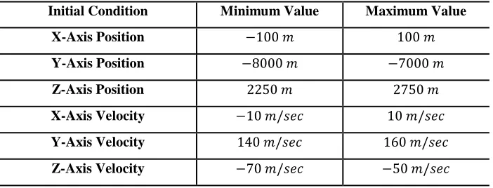
Importantly, by utilizing reinforcement learning, the guidance algorithm parameters are optimized in a stochastic environment. That is, the guidance parameters are being learned to be optimal over a range of starting condition and in an environment that accounts for sensor or navigation errors. By including these in the learning process, the resulting parameters will not only provide optimality from a fuel consumption standpoint, they will also include robustness to initial state perturbations and sensor errors, which is not accounted for in the given optimal trajectory seen in Figure 2 and 3. The reinforcement learning simulation used to calculate the utility of a certain combination of parameters uses conditions which are very similar to those provided in the previous section. The initial wet mass of the spacecraft remains 1900 kg. The range of initial conditions employed to learn the optimal guidance parameters are reported in Table 2. Each of these values are uniformly distributed between the respective minimum and maximum values, providing a total of 144 samples that are used to learn an optimal set of parameters. Further, these simulations included uncertainties of and in position and velocity, respectively, which are provided to the guidance algorithm to simulate sensor noise when estimating the current state of the spacecraft. Finally, the utility function, which is determined at the end of the simulation of each sample, which is used in order to determine which set of parameters is optimal, was chosen to be quadratic:
( ) ‖ ‖ ‖ ‖ ( ) (48)
Here, the terms ‖ ‖ and ‖ ‖ represent the final position and velocity errors that result from the chosen guidance parameters, represents the difference between the final lander mass resulting from the chosen parameters and the final mass computed by numerically solving the open-loop optimal landing problem as discussed in the previous section. Additionally,
and represent the parameters that weight the importance of each of their respective terms. Essentially, this utility function is attempting to minimize the residual error of the guidance law as well as minimizing the fuel usage over the given set of initial conditions. The values are selected as a trade-off between the importance of errors in position, velocity and fuel mass. It was found via numerical simulations that velocity has the highest contribution to the overall error and required a higher weight. Final weights were selected to be , and .
previous iteration: if the new utility is lower, the set of guidance gains is retained. Otherwise, the new set of gains is replaced by the one at the previous iteration. The process continues until convergence. More specifically, the algorithm is declared to have converged when the variation in utility over the current epoch falls below a specified threshold.
Table 2. Initial Condition Range for Reinforcement Learning Parameter Optimization
Initial Condition Minimum Value Maximum Value
X-Axis Position
Y-Axis Position
Z-Axis Position
X-Axis Velocity
Y-Axis Velocity
Z-Axis Velocity
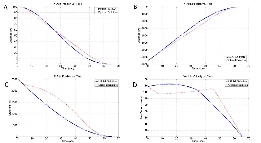
The results of the RL optimization are captured in Table 3. Importantly, the final time of the simulation determined by reinforcement learning is very close to the value determined by the optimal solution, .
Table 3. Optimal Parameter Results of Reinforcement Learning
Figure 4. Comparison of Reinforcement Learning Optimized MSSG System Trajectories to Optimal Solution
Figure 5. A) Thrust Magnitude and B) Lander Mass Histories Comparing Optimal Solution to Reinforcement Learning Optimized MSSG
[image:19.612.105.536.330.444.2]Table 4. Comparison Between the Open-Loop Fuel-Optimal Guidance and the Reinforcement Learning Optimized MSSG Guidance (Propellant Mass)
Optimal (GPOPS)
RL Optimized MSSG
Mass of Propellant/Optimal
Value 1 1.032
Mass of Propellant
Monte Carlo Analysis of Optimized MSSG
In order to further validate and analyze the behavior of the guidance algorithm employing the learned MSSG guidance parameters, a Monte Carlo analysis has been performed to test the system under off-nominal conditions. The Monte Carlo analysis has been conducted by running 1000 simulations of the MSSG algorithm in the described 3-DOF framework (Eq. (1)-(10)). In simulating the MSSG-guided powered descent, we included additional perturbing accelerations and navigation errors to simulate a more realistic descent and landing. Table 5 shows the parameters used in the simulations, as well as their dispersions. All values are assumed to follow a normal (Gaussian) distribution described by their respective means and standard deviations. The MSSG parameters and gains are selected to be exactly those reported in Table 3. The nominal case for the Monte Carlo simulation is the same as seen in the previous analysis. Furthermore, the main thruster mass-flow rate is perturbed using a normal distribution which is set assuming an upper value of 10% deviation from the mean value. An additional random acceleration (Gaussian distribution with zero mean and 10% standard deviation) has been added to account for unmodeled dynamics.
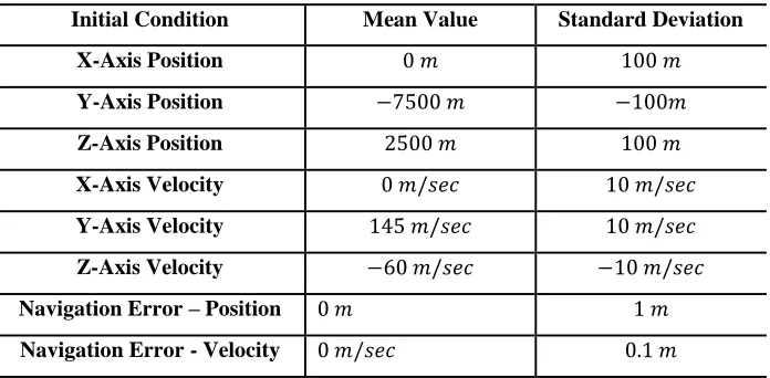
Table 5. Initial Condition Dispersions for Monte Carlo Simulation
Initial Condition Mean Value Standard Deviation
X-Axis Position
Y-Axis Position
Z-Axis Position
X-Axis Velocity
Y-Axis Velocity
Z-Axis Velocity
Navigation Error – Position
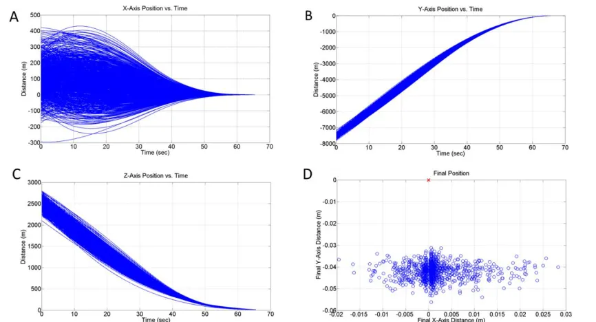
[image:20.612.134.482.417.588.2]Figure 6. Monte Carlo Simulation Results: A) X-Axis Position; B) Y-Axis Position; C) Z-Axis Position; and D) Final Landing Location Dispersion
Figure 7. Monte Carlo Simulation Results: A) X-Axis Velocity; B) Y-Axis Velocity; C) Z-Axis Velocity; and D) Velocity Magnitude
and off nominal conditions. Figures 8 and 9 show that the residual errors in position and velocity are very close to zero. The statistics of the Monte Carlo simulations are reported in Table 6.
Figure 8. Monte Carlo Simulation Results: A) X-Axis Miss Distance; B) Y-Axis Miss Distance; and C) Magnitude of Miss Distance
[image:22.612.106.539.371.613.2]Table 6. Monte Carlo Simulation Result Statistics
Initial Condition Mean Final Value Standard Deviation
X-Axis Position
Y-Axis Position
Z-Axis Position
X-Axis Velocity
Y-Axis Velocity
[image:23.612.105.532.248.391.2]Z-Axis Velocity
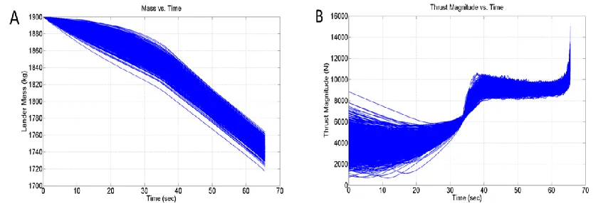
Figure 10. Monte Carlo Simulation Results: A) Lander Mass History; and B) Thrust Magnitude History
Clearly the performance of the algorithm with the given parameters is quite good. Figure 6d shows that the final miss distance is very near zero for all cases, demonstrating the accuracy of the algorithm with the optimized parameters. However, as can be seen in Figure 9, and Table 6, some cases did contain significant residual velocity error. The residual final velocity has a maximum value of , which is mostly in the direction (Figure 9c). However, most of the cases exhibit residual velocity errors much smaller than the worst case. This error can be attributed in part to the amount of training that was performed within the reinforcement learning environment. Importantly, the MSSG parameters were determined for the nominal initial condition as opposed to a set of parameters that work best over the entire space defining all possible initial conditions. It is likely that the worst case was very near the edge of the design space that was used in the learning environment, and as such further training will likely remove these errors.
final altitude achieved in the reinforcement learning environment was seen to be 9.57 meters. Consequently, a small undershoot in the y-axis position is expected, and if the Monte Carlo were run with this cutoff altitude, the bias removal from the results would be expected.
CONCLUSIONS AND FUTURE WORK
A non-linear guidance algorithm for planetary pinpoint landing using Higher Order Sliding Mode (HOSM) control is presented and analyzed. In previous work, the algorithm was developed and applied as possible guidance scheme for close-proximity operations around small bodies. It was theoretically proven to be globally stable under the assumption that an upped bound for the perturbing accelerations is known. Moreover, the algorithm was demonstrated to be both robust and accurate under perturbations and unmodeled dynamics arising in operating in uncertain environments typically found around small-bodies. Here, the MSSG algorithm is revised and extended for the general problem of terminal landing guidance for large planetary bodies. Whereas the stability properties and robustness are preserved also for the planetary landing case, the closed-loop guidance algorithm is generally shown to be suboptimal from a fuel consumption standpoint. Indeed, a comparison between a numerically computed fuel-efficient open-loop guidance solution and the MSSG algorithm has been executed. The comparison highlights the need to tune the required five guidance gains to achieve competitive accuracy and fuel efficiency. The RL framework has been employed to learn the guidance gains that generate a close-to-optimal behavior for the proposed guidance algorithm. Indeed, the resulting implementation of the reinforcement learning scheme has numerically generated a set of guidance parameters that bring the performance of the MSSG algorithm very close to that provided by an optimal open-loop solution while maintaining its inherent feedback nature. Further, the algorithm does not require the generation of a reference trajectory, and as such is more flexible under off-nominal conditions and perturbations. The features of accuracy, flexibility, and good fuel usage make the RL-tuned MSSG algorithm very applicable for future planetary missions that require pin-point landing.
that are shaped by changing the guidance gains . For the general landing close-loop guidance problem, such gains can be learned as function of the state to shape the trajectory as dictated by mission-specific needs (e.g. altitude angle or glide-slope constraint).
Future work for the MSSG algorithm include a) inclusion of additional constraints in the reinforcement learning process, including glide-slope constraints and attitude/thrust constraints b) shifting the paradigm of one set of guidance parameters to that of a more adaptive approach, which will allow the reinforcement learning algorithm to learn an optimal set of guidance parameters that update during the descent phase, and c) the application of reinforcement learning of the MSSG algorithm to other scenarios, including asteroid proximity operations and Mars hypersonic reentry and terminal powered landing guidance. These additional features and analysis will allow the MSSG algorithm to be further refined and analyzed under more strenuous conditions and provide further understanding into the true application of the algorithm for future mission architectures.
REFERENCES
[1] A. A. Wolf, J. Tooley, S. Ploen, M. Ivanov, B. Acikmese, K. Gromov, Performance Trades for Mars Pinpoint Landing, IEEE Aerospace Conference Proceedings, March 2006, IEEE-1661, March 2006.
[2] A. Wolf, E. Sklyanskly, J. Tooley, B. Rush, Mars Pinpoint Landing Systems Trades, AAS/AIAA Astrodynamics Specialist Conference Proceedings, AAS 07-310, August 19-23, 2007
[3] Phinney, W.C., Criswell, D., Drexler, E., Garmirian, J. “Lunar Resources and Their Utilization”, Space-Based Manufacturing from Nonterrestial Materials, AIAA p. 97-123, 1977.
[4] A. D., Steltzner, D. M., Kipp, A., Chen, P. D.,Burkhart, C. S., Guernsey, G. F., Mendeck, R. A., Mitcheltree, R. W., Powell, T. P., Rivellini, A. M., San Martin, D. W., Way, Mars Science Laboratory Entry, Descent, and Landing System, IEEE Aerospace Conference Paper No. 2006-1497, Big Sky, MT,(2006).
[5] G. Singh, A. SanMartin, and E. Wong. Guidance and control design for powered descent and landing on Mars.
Aereospace Conference IEEE, 2007.
[6] A. R., Klumpp, A Manually Retargeted Automatic Landing System for the Lunar Module (LM), Journal of Spacecraft and Rockets, Volume 5, Issue 2, 1968, pp 129-138.
[7] A. R., Klumpp, Apollo Guidance, Navigation, and Control: Apollo Lunar-Descent Guidance, Massachusetts Inst. of Technology, Charles Stark Draper Lab., TR R-695, Cambridge, MA, June 1971.
[8] A. R., Klumpp, Apollo Lunar Descent Guidance, Automatica, Volume 10, Issue 2, 1974, pp. 133-146.
[9] U., Topcu, J., Casoliva, and K., Mease, Fuel Efficient Powered Descent Guidance for Mars Landing, AIAA Paper 2005-6286, 2005.
[10] F., Najson, and K., Mease, A Computationally Non-Expensive Guidance Algorithm for Fuel Efficient Soft Landing, AIAA Guidance, Navigation, and Control Conference, San Francisco, AIAAPaper 2005-6289, 2005.
[11] B., Acikmese, and S. R., Ploen, Convex Programming Approach to Powered Descent Guidance for Mars Landing, Journal of Guidance, Control, and Dynamics, Vol. 30, No. 5, 2007, pp. 1353–1366.
[12] C. D’Souza, An Optimal Guidance Law for Planetary Landing, AIAA Guidance, Navigation, and Control Conference, AIAA Paper 1997-3709, 1997.
[13] D. A., Benson, G. T., Huntington, T. P., Thorvaldsen, and A. V., Rao, Direct trajectory optimization and costate estimation via an orthogonal collocation method. Journal of Guidance, Control, and Dynamics, 29(6), 2006, 1435-1440.
[14] J. F., Sturm, Using SeDuMi 1.02, a MATLAB Toolbox for Optimization Over Symmetric Cones, Optimization Methods and Software, Vol. 11, No. 1, 1999, pp. 625–653.
[16] Y., Nesterov, and A., Nemirovsky, Interior-Point Polynomial Methods in Convex Programming, SIAM, Philadelphia, PA, 1994.
[17] L. Blackmore, B. Acıkmese, and D. P Scharf. Minimum landing error powered descent guidance for Mars landing using convex optimization. AIAA Journal of Guidance, Control and Dynamics, 33(4):1161–1171, 2010.
[18] A., Levant, Construction Principles of 2-Sliding Mode Design, Automatica, Vol. 43, No. 4, (2007), pp. 576– 586.
[19] Levant, A., Sliding order and sliding accuracy in sliding mode control. International Journal of Control, 58(6), 1993, 1247–1263.
[20] A. Levant, Higher-order sliding modes, differentiation and output feedback control. International Journal of Control, 76(9/10), (2003), 924–941.
[21] Levant, A. Homogeneity approach to high-order sliding mode design. Automatica, 41(5), (2005a). 823–830. [22] Levant, A., Quasi-continuous high-order sliding-mode controllers. IEEE Transactions on Automatic Control,
50(11), (2005b), 1812–1816.
[23] Y. B., Shtessel, & I. A., Shkolnikov, Aeronautical and space vehicle control in dynamic sliding manifolds. International Journal of Control, 76(9/10), 1000–1017, 2003.
[24] M., U., Salamci, M., K., Ozgoren, S., P., Banks, Sliding Mode Control with Optimal Sliding Surfaces for Missile Autopilot Design, Journal of Guidance, Control and Dynamics, Vol. 23, No. 4, 2000.
[25] Y., Shtessel, and C., Tournes, Integrated Higher-Order Sliding Mode Guidance and Autopilot for Dual-Control Missiles, Journal of Guidance, Control and Dynamics, Vol. 32, No. 1, 2009.
[26] C., Tournes, Y., Shtessel, I., Shkolnikov, Missile Controlled by Lift and Divert Thrusters Using Nonlinear Dynamic Sliding Manifolds, Journal of Guidance, Control and Dynamics, Vol. 29, No. 3, 2006.
[27] A., Koren, M., Idan, O., M., Golan, Integrated Mode Guidance and Control for a Missile with On-Off Actuators, Journal of Guidance, Control and Dynamics, Vol. 31, No. 1, 2008.
[28] R. Furfaro, S. Selnick, M. L. Cupples and M. W. Cribb, Non-Linear Sliding Guidance Algorithms for Precision Lunar Landing, in Advances in the Astronautical Sciences, Volume 140, Proceedings of the 21st AAS/AIAA Space Flight Mechanics Meeting held February 13-17, 2011, New Orleans, Louisiana.
[29] Furfaro, R., Cersosimo, D., Wibben, D.R., “Asteroid Precision Landing via Multiple Sliding Surfaces Guidance Techniques,” Journal of Guidance, Control, and Dynamics, Vol. 36, No. 4, 2013, pp. 1075-1092.
[30] R. Furfaro, D. O., Cersosimo and J. Bellerose, Close Proximity Asteroid Operations using Sliding Control Modes, Proceedings of the annual AAS/AIAA Space Flight Mechanics Conference, AAS 12-132, Jan 31-Feb 4, 2012, Charleston, Louisiana.
[31] N., Harl, and S., N., Balakrishnan, Reentry Terminal Guidance Through Sliding Control Mode, Journal of Guidance, Control and Dynamics, Vol. 33, No. 1, January–February 2010.
[32] Sutton, R., Barto, A., Reinforcement Learning, MIT Press, 1998, pp. 100-103. [33] Slotine, J., and Li, W., Applied Nonlinear Control, Prentice Hall, 1991.
[34] T. L., Vincent, & W. J. Grantham, Nonlinear and optimal control systems. New York: Wiley, 1997.
[35] L. Fridman. An averaging approach to chattering. IEEE Transactions on Automatic Control, 46(8), 2001, 1260–1265.
[36] A. V., Rao, D. A., Benson, C., Darby, M. A., Patterson, C., Francolin, I., Sanders, et al. Algorithm 902: GPOPS, a MATLAB software for solving multiple phase optimal control problems using the Gauss pseudospectral method. ACM Transactions on Mathematical Software, 37(2), 2010, 22:1-22:39.
[37] P.E. Gill, M.A. Saunders, and W. Murray. SNOPT: An SQP algorithm for large scale constrained optimization. Technical Report NA 96-2, University of California, San Diego, 1996.
[38] Amato, M., Garvin, J. B., Burt, I. J., Gardner, T., & Karpati, G. Lower-Cost, Relocatable Lunar Polar Lander and Lunar Surface Sample Return Probes, Paper for the Iinternational Planetary Probe Workshop 2010.