An agent-based implementation of hidden Markov models for gas turbine condition monitoring

1

An Agent-based Implementation of Hidden Markov

Models for Gas Turbine Condition Monitoring

A. D. Kenyon,

Member, IEEE

, V. M. Catterson,

Member, IEEE

,

S. D. J. McArthur,

Senior Member, IEEE

, J. Twiddle.

Abstract—This paper considers the use of a multi-agent sys-tem (MAS) incorporating hidden Markov models (HMMs) for the condition monitoring of gas turbine (GT) engines. Hidden Markov models utilizing a Gaussian probability distribution are proposed as an anomaly detection tool for gas turbines components. The use of this technique is shown to allow the modeling of the dynamics of GTs despite a lack of high frequency data. This allows the early detection of developing faults and avoids costly outages due to asset failure. These models are implemented as part of a MAS, using a proposed extension of an established power system ontology, for fault detection of gas turbines. The multi-agent system is shown to be applicable through a case study and comparison to an existing system utilizing historic data from a combined-cycle gas turbine plant provided by an industrial partner.

Index Terms—Gas turbines, Fault detection, Hidden Markov models, Gaussian distributions, Condition monitoring, Multi-agent system

I. INTRODUCTION

Failure of a component within a generation plant may require the unit to be taken off-line, and it may remain unable to generate electricity for an extended period of time. This can incur a loss of earnings and lasting damage to the utility’s reputation. For these reasons the condition monitoring of assets and the timely detection of faults is an important aspect of maintaining a generation fleet. This paper introduces an approach involving the use of several hidden Markov models, implemented as intelligent agents, to capture the underlying behavior of the components of gas turbines, allowing the modeling of the turbine characteristics without the need for high frequency data. The algorithm is shown to allow effective fault-detection capability through a comparison with an exist-ing condition monitorexist-ing system usexist-ing data from the same plant.

The implementation of the hidden Markov models as intelli-gent aintelli-gents allows the construction of a multi-aintelli-gent condition monitoring system. The system utilizes and extends an existing power engineering ontology to maintain compatibility with current and future systems in the domain. The flexibility of the system is demonstrated through the deployment of additional algorithms complementary to the HMM-based approach.

HMMs have been used extensively in speech recognition [1]. In cases where they have been used to model dynamic systems a high sampling rate has been available [2] [3], often several samples a second. The proposed system is unique in applying HMMs to an application where the sampling interval is several minutes. An example is provided to show that HMMs are still capable of fault detection under these

conditions, with performance comparable to or exceeding those of existing techniques. The use of multiple diagnostic models, in a modular system, is not unusual [4] [5]. However, the use of MAS technology using freely available standards increases the potential for new innovative algorithms and evidence combination techniques to be incorporated in to the system.

Section II provides a brief overview of gas turbine con-dition monitoring and the associated challenges. Section III summarizes the principles of HMMs, and explains why they are used for this application. Section IV shows an example of HMMs trained on combustion data with a low sample rate, and compares the performance of the HMMs to an existing commercial system, and shows superior performance. Section V describes the standards and technologies utilized to deploy a multi-agent system. Implementation details are provided for a prototype system incorporating several algorithms as intelli-gent aintelli-gents, including HMMs for the main GT subsystems, for condition monitoring of real plant data. This includes details of the operation and communications between agents. Section VI concludes with a summary of the paper’s findings.

II. GASTURBINECONDITIONMONITORING

Gas turbine condition monitoring is a broad and mature field, covering not only techniques developed for the power industry, but also for the aero-engine market. GT plant mon-itoring systems can still take many forms, owing to the large number of potential sources of failure [6]. Often a plant-wide database may exist consisting of relatively low frequency data, with sampling rates of several seconds. Data from this source can be useful, but it is difficult to capture the dynamic behavior of a gas turbine rotating at high speed without a high sampling rate. This often results in a second system being employed using higher frequency readings to better capture the dynamic behavior of the turbine. However, this will be only for a limited number of specific variables, typically vibration, and requires separate analysis from the other data. There are automated approaches involving signal analysis of vibration or other high-frequency data. This includes using Fourier or Wavelet transforms of the captured data, examples include Beran [7] and Symbolic Dynamic Filtering [8].

detection capability, but little capability to detect precursors to pending faults [9]. SBM has been shown to be effective by modeling the similarity of data vectors to existing training examples [10]. This means that it is potentially vulnerable to variations caused by seasonal or operational conditions. While it is possible to mitigate this through the use of a large and up-to-date training set, it would be preferable to have a model that reflects the underlying behavior, and is therefore resilient to such variations.

HMMs have been successful in capturing the underlying states of other types of dynamic systems [2]. HMMs have been shown to be effective for anomaly detection of other electrical assets such as transformers [11]. This technique arose from the fundamental work undertaken by Fox et al [12]. HMMs have proven themselves, with several variations of HMM applied to rotating machinery [13] [14] [15]. However, none of these have been applied to low-frequency data from power GTs.

Many techniques have found their way into composite con-dition monitoring systems. Examples include AMODIS [4], which includes tools for monitoring entire plants, and TI-GER [5] which is focused specifically at GT monitoring. Regardless of the scope of the assets focused on, systems such as these typically cover the processes of data acquisition, pre-processing, anomaly detection, fault isolation and fault diagnosis. Systems may apply only a single algorithm to each task, or may combine several in an effort to minimize the weaknesses of individual techniques. In the case of more spe-cialized systems like TIGER, the turbine may be divided into subsystems of related variables. Such systems are extensible, with additional algorithms being added in or existing ones updated or replaced. None of these systems use HMMs to model the dynamics of the system as proposed in this paper and therefore can miss anomalous behavior short of failure. However, their extensibility and modularity are considered a requirement for any solution proposed in this paper. To provide such capabilities, the HMM-based algorithm is deployed as an intelligent agent within a prototype multi-agent system.

III. HIDDENMARKOVMODELS

HMMs were chosen due to their potential to model the underlying dynamics of a system by way of their hidden states, in expectation that this would allow them to outperform other techniques in timely anomaly detection. The following section summarizes the theory behind HMMs.

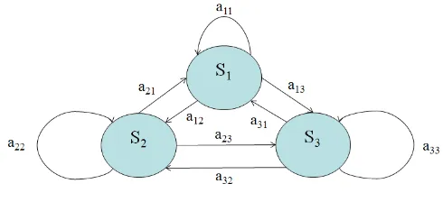
HMMs are a type of probabilistic model [16]. The principle of a HMM is that given a set of observations, it is possible to derive the most likely set of underlying states and the associated probability of transitioning between those states. In this way, a HMM may model the internal behavior of a system based on only that system’s inputs and outputs. A simple HMM is shown is shown in Figure 1.

Figure 1 shows the principle of a three state HMM, with the states given the designations S1,S2 andS3. The state trans-ition probabilities are represented by the nine “a” variables. For a HMM with S states, these probabilities are stored in a SxS state transition matrix, usually called A, where the aij

element represents the probability of transitioning from Si to

Figure 1. A 3 State HMM

Sj. A HMM also contains a vector with the probabilities of

starting (t= 0) in a particular state, represented by the vector π, of lengthS.

Variations exist on how a HMM represents the probabilities of observations [1]. Regardless of how it is calculated or stored, bj(O) represents the probability of the observation

O, while in state j. If the inputs to the model are discrete, bj(O), is a scalar value between 0 and 1. When combined,

the probabilities of all observations must be 1 for each state. If there areO possible discrete observations, the probabilities are stored inB, aSxOobservation matrix. As the data for the GT application is in the form of continuous values, in order to use a discrete HMM it would be necessary to cluster or classify the values in some way to derive discrete observations.

In order to use continuous inputs directly,O may not rep-resent a classifier symbol as is the case with discrete HMMs, but rather a real value. To represent the probability of all possible values it is necessary to use a continuous probability density function, rather than an observation matrix. This is accomplished by combining many Gaussian distributions in a Gaussian mixture model (GMM). This paper will refer to this type of model as a mixture HMM (MHMM). Equation 1 below shows a 1-dimensional Gaussian function, where x is the input,µis the mean andσ2_{is the variance.}

g(x|µ, σ2) =√ 1

2πσ2e −(x−µ)2

2σ2 (1)

The Gaussian distributions are combined using a mixture weight to form an approximate distribution. Each state has its own GMM. As the continuous input is being fed directly to the MHMM, x is equivalent to an observationO. Therefore, if bj(O)once again means the probability of the observation O

while in statej,M is the number of mixtures, andcjm is the

mixture weight for themth mixture of statej, the probability is given by:

bj(O) = M

X

m=1

cjmg(O|µjm, σ2jm), O

X

bj(O) = 1 (2)

(weight) matrix, a SxMxD mean matrix, and a SxMxDxD covariance matrix in place of a observation matrix [3]. This allows the construction of any value ofbj(O). The model, λ,

may now be fully defined:

λ= (A, C, M,Σ, π) (3)

A. Training and Testing a HMM

The output of a HMM is the maximum probability of a particular sequence of observations given the model para-meters. As the probability is a function of both the state transition probability and observation probability this is not straightforward to calculate. This complicates training and testing of the HMM. The solutions are described elsewhere [1]. What follows is a brief summary of how the HMMs were trained and tested for this application.

Training requires the HMM to “learn” the behavior it is presented with during the training period. This requires some form of algorithm to adjust the HMM parameters so as to maximize the output probability value for behavior similar to that seen during training. There is no analytic way of de-termining the optimal values for the HMM parameters, so the expectation maximization algorithm [17] [18] was used. This also incorporated the forward-backward procedure [19] [20], which utilizes induction to reduce complexity, in order to keep training time reasonable. While this is not guaranteed to find the global maximum, providing only local maximum, it is an accepted practical solution [1].

Testing is addressed by finding the maximum probability of the observations provided as test data. This is a potentially computationally expensive task if calculated directly [1]. The forward-backward procedure was once again applied to reduce the required number of calculations. This allowed the time taken to calculate output probability values to be greatly reduced making on-line testing of larger models possible where it would otherwise not be possible.

B. Interpreting the model output

When considering the output probabilities it is necessary to use a logarithmic scale. This is because, being a probability, the output of the HMM is continually multiplied by values less than 1. Figure 2 shows that this makes it difficult to interpret the output after only 50 observations of a 100 observation sequence. By using a log scale the curve becomes a roughly straight line for normal behavior.

The log scale also makes it much easier to pick out anomalies (which present themselves as deviations from the trajectory of normal behavior) and allows easier visualization of the results. In general, when considering the output of the HMM, the term “likelihood” is used in literature [1] rather than “probability”, and as the log scale is used, this is then termed the “log-likelihood”(LL).

A useful way to visualize the results of a HMM is to plot several sequences simultaneously. This allows a “cone” of normality to be built up, allowing sequences that diverge from normal behavior to be easily identified. However, it can also be desirable to plot the LL over a long period of time. In

Figure 2. Linear vs Log Scales for Normal and Abnormal Sequences

this case, only the final LL value is presented to the user. A comparison of the two visualizations is provided in Figure 3.

Figure 3. Comparison of Cone and Final Log Likelihood Plots

IV. COMBUSTIONMODELING USINGHIDDENMARKOV

MODELS

Hidden Markov models were used to model the gas turbines of a single unit of a CCGT. This contained two single-spool gas turbines burning natural gas, each coupled via a shaft to its own generator. The exhaust gases from each turbine also feed separate heat recovery steam generators. The steam produced is then used to power a single steam turbine and its coupled generator.

A. Available Data

operational turbines. This data is sampled every 10 minutes. While frequency-based vibration monitoring of the GTs is performed by the utility, this was not available for use with the proposed algorithms.

The gas turbines are divided into 5 variable groups for modeling by the existing condition monitoring system. All include the GT load and ambient temperature at the plant. More specifically, the variable groups are:

1) Compressor: 19 variables consisting of mostly pressures and temperatures around the axial-flow compressor. 2) Combustion: 46 variables consisting of a combustion

chamber temperature vector of 31 readings, and addi-tional input and output temperatures and pressures. 3) Fuel Flow: 21 variables including servo feedback

read-ings, fuel temperature and pressures, and some GT operational parameters.

4) Mechanical: 30 variables primarily concerning ball bear-ing temperature and vibration measurements.

5) Wheelspace: 21 variables, all thermocouple readings. At least 2 sensors before and after each turbine stage, plus additional temperatures before and after turbine wheelspace.

These variable groupings are carried over to the models presented in this paper. This is in order to allow a direct comparison of results between the existing and proposed sys-tems. Due to the presence of known faults strongly correlated to combustion, the results presented in this section focus on those models. However, the prototype system arising from the research reported in this paper (described in Section V) contains models for all variables groups and in this regard is fully equivalent to the existing system.

The following sections document the process followed in order to apply probabilistic models to the GT monitoring domain. A process of data mining [21] was used to drive the preparation and analysis of the available data, before training and experimentation with MHMMs began in order to find a suitable model.

B. Data Preparation

Data taken from the gas turbines during steady-state oper-ation was used for analysis. This was motivated primarily by the abundance of such data. This would provide ample training data, a pre-requisite when using a data-based technique [22] such as HMMs. Data taken from periods outside steady-state operation was considered, but was less common and more intermittent. Attempting to visualize this data showed that the scarcity and brevity of these occurrences would make the trending of GT behavior, and therefore the detection of degradation in performance, more difficult.

Any captured data may have invalid inputs, which may be due to a faulty sensor or a data line failure. These must be flagged and removed if necessary as part of the data cleaning process. If the application is for only a particular operational state it will also be necessary to filter the data to remove inappropriate data. As HMMs are required to model transitions over time, simply removing individual data vectors without regard for continuity was not an option. Because of this a

decision was reached to only consider contiguous observation sequences of valid on-load inputs.

The data was sampled every 10 minutes, as provided by the utility. Existing systems used by the utility group data into 3 hour blocks. In line with this the HMM grouped the samples into observation sequences of length 20, resulting in a period of 3 hours and 20 minutes.

Data reduction techniques were considered, but this would require an additional stage before the HMM that would make it more difficult to evaluate the HMM performance. It was also desirable to use the same range of inputs as the existing system, to provide a more direct comparison. For similar reasons the use of a discrete HMM was discounted as this would have required a similar preprocessing stage in the form of a classifier or clusterer. By its nature a classifier could reduce the sensitivity of the HMM to small changes in inputs. While this may be a positive attribute for some fault diagnosis systems, the desire for the HMMs to be able to show gradual degradation over long periods of time makes this approach poorly suited to this application. Due to the desire to provide a clearer indicator of gradual degradation a continuous HMM technique was selected for implementation and testing.

C. Processing Results

For simplicity and transparency, and the need to view a timeline to match utility requirements, only the final LL value of a sequence is considered when evaluating the performance of the algorithm. Considering each LL cone separately would be a time consuming process. However, the prototype system contains the capability for the user to isolate any point on the final LL graph and view the full LL cone if they need further information.

When evaluating the performance, it is necessary to define how to interpret the HMM results. The HMM’s LL value does not have a hard threshold as not only the absolute LL value but also the general trend and any dips or divergence from that trend all had to be considered. A low absolute value could be considered a persistent fault, or could simply be a slight change in behavior due to a maintenance procedure. The trend is useful as this can often indicate degradation which can lead up to a failure. Finally, a “dip” outside of this trend can often indicate a fault has already occurred. Considering all three of these metrics is potentially more complicated to automate than a simple threshold-based approach. In this paper all the results have been interpreted by hand. It is intended that the next stage of work will incorporate automated techniques to analyze the LL plots.

D. Adjusting the Model

With the concept of MHMM-based anomaly detection es-tablished, the next step is to define a satisfactory model architecture. Because of the ‘black box’ nature of HMMs the optimal number of states and observations/mixtures for a HMM is difficult to calculate exactly. It is also possible that the potential accuracy of a larger model is offset by the increased computational complexity that this requires. There is no hard-and-fast rule for determining the best model parameters, so it is necessary to rerun tests with different models.

Figure 4. Comparison of Model Sizes

The first round of tests concentrated on the size of the model and varied the number of states and mixtures. When considering both fidelity and computational expense, a good compromise was found using 10 states and 8 mixtures. Figure 4 shows that a smaller model shows a smaller range of log-likelihood levels across the testing period, representing a loss of resolution. While smaller models did decrease training and testing time, this was not sufficient justification for a loss in model effectiveness.

Larger models increased the dynamic range. This is due to the larger number of mixtures and states allowing the model to more closely fit the training data and, in the case of mixtures, reducing the Gaussian variance. This would result in abnormal values having much lower LL values. While this is generally desirable, it is possible that individual values can become extremely low, beyond that which may be represented in computer memory as a finite value. This was the case with some of the larger models and resulted in more of an on-off anomaly detection capability. This was not the desired outcome and for this application smaller models were deemed more appropriate.

Further experimentation was carried out by varying the length of the observation sequences fed into the model. Figure 5 shows that the smaller sequence has generally higher LL values. This is because LL is cumulative. While it would also increase the frequency of model output, the difference between normal and abnormal behavior is once again compromised when looking at the final LL values. Conversely, when tested

Figure 5. Comparison of testing using different observation sequence lengths.

against sequences with greater than 20 observations the num-ber of sequences dropped and, as the LL values decreased uniformly, did not display improved fidelity or dynamic range that would assist in determining the presence of anomalies. These results have led to the conclusion that the original sequence length of 20 observations is adequate. As this is also in line with the utility’s practice of analyzing 3 hours of data at a time this was used for all subsequent tests.

E. Validation

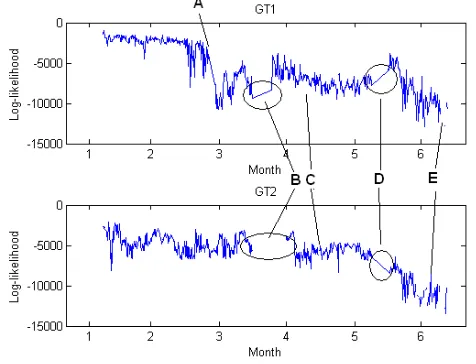
After some preliminary tests, promising results were ob-tained for both turbines using models with 10 states and 8 mixtures, using the sequence length of 20. These results are shown in Figure 6.

Figure 6. Initial test using MHMM on combustion data

It was attempted to correlate the level, trends, dips and variations in LL values shown in Figure 6 to trips and other factors that may explain them.

from the utility, this is attributed to low level faults that would affect previous data (including training data), that were fixed during month 2. This would affect the behavior of the turbine and would be visible as a drop in LL.

While both turbines experience an outage starting in the middle of month 3 for routine maintenance, GT2 appears to start later after the month 3 shutdown (B). In fact this is due to several trips running up to end of the month. It was rarely up to base load long enough for a complete sequence and there were negative infinity LL values (suggesting extremely unusual behavior) when it was.

Both turbines show a slight drop in month 4 which cor-relates with combustion retuning changing the GT behavior slightly (C). There is an outage in month 5 (D), which shows GT1’s LL temporarily increase. This is attributed to maintenance performed on GT1 during this time. The values of both GT1 and GT2 then gradually drop off until increasing number of negative infinity values begin to occur (E). This is due to a combination of low level faults and a particularly large seasonal variation in temperature and pressure values.

F. Generalizing the Model

As one of the advantages of HMMs is the ability to learn underlying behavior, there is a possibility of deriving a general turbine model based on training data from multiple turbines. A model was trained using the combined training data of both GT1 and GT2. It should be stressed that this is limited to only two turbines of the same manufacturer and model, and as such further data and testing would be required to develop a true general GT model. In this case, it is useful because it provides a means to deploy a model for a known GT type even when no data is available to train a specific GT, such as when a new turbine is installed.

Figure 7. Comparison of GT-specific models to a model trained on data across both turbines

The results in Figure 7 show that the model with a combined training set produces results close to the individual models, particularly noticeable in the GT1 results. Interestingly, the general model actually shows a higher LL for GT2 than the

GT2-specific model, but does still show degradation until the lower values towards the end of the time period. This would suggest that the dedicated model is more sensitive to the change in operational values due to water washes and other maintenance.

The results suggest that the general model is still able to continue effective anomaly detection. Despite the wider ranges of values, the general model has successfully learned the behavior of a turbine, even if the values vary slightly depending on the specific turbine. The use of a general model may make it possible to monitor a new turbine until sufficient data is available to allow a more sensitive turbine-specific model to be deployed.

G. Results

With the MHMM trained, its performance alongside the ex-isting condition monitoring system was considered. The time and date of successfully detected anomalies were compared. The comparison focuses on major confirmed anomalies. A side by side comparison shows the HMM stands up well to the results from the existing system. This is particularly impressive as the training data contains only the original data — without the additional data added to the deployed model throughout the comparison period and beyond.

Table I

PERFORMANCE COMPARISON OFMHMMVS.EXISTING SYSTEM.

GT Month Events MHMM Existing System Similar

GT1 1 2 2 0 0

2 2 1 1 0

3 3 1 1 1

4 1 1 0 0

Total 8 5 2 1

GT2 1 2 1 1 0

2 5 1 1 3

3 2 2 0 0

4 N/A N/A N/A N/A

Total 9 4 2 3

Table I shows a breakdown of the number of anomalies recorded during a 4 month period. The “MHMM” column shows the number of times the MHMM detected an anomaly before the existing system, or detected an anomaly which the existing system did not. The “Existing System” column counts the cases where the reverse is true, and the “similar” column counts the number of times where anomalies were detected within a similar timescale by both. Data was unavailable for GT2 during month 4.

The results show that each system picks up different an-omalies, with the MHMM identifying more than the existing system. While each individual system missed anomalies, no anomaly failed to be detected by one of the systems, suggest-ing that an optimal system would use both along with some means of corroboration.

H. Applying HMMs to other subsystems

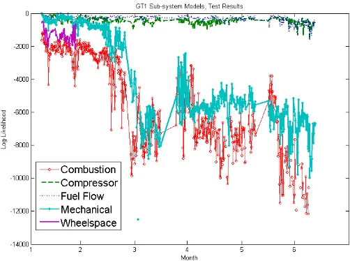
MHMMs were trained to the other variable groups (see Section IV-A) for GT1. Figure 8 shows the results.

Figure 8. The log-likelihoods of all sub-system across the test period for GT1

The results show a number of interesting similarities between the sub-systems. The compressor and fuel flow appear to display similar values. While the mechanical results starts with similar values to the compressor and fuel flow models, it drops following the maintenance performed in month 2, at the same time as the dip in the combustion results (Figure 6, point A). From then on it displays results across the test period similar to the combustion model. The compressor and fuel flow models remain relatively unaffected by this maintenance.

The Wheelspace model returns negative infinity values following the first month. This suggests an event that affected the wheelspace variables and changed the underlying behavior and relationships. The change occurs at the same time as the second combustion event in month 1 (see Table I). This suggests that while the combustion model picked up this anomaly, the effect on wheelspace was far greater and more persistent.

The other subsystems all show a drop off starting in month 5, leading to negative infinity values as the turbine behavior deviates significantly from the model.

These results suggest that training HMMs on other sub-systems is practical, and can provide additional information about detected anomalies. This necessitates a mechanism to allow several HMMs to be deployed and interpreted concur-rently. The following section proposes a multi-agent system to meet this requirement.

V. IMPLEMENTATION AS AMULTI-AGENTSYSTEM

After the algorithm was successfully applied to GT data, a prototype on-line system incorporating the technique was developed. The system was required to allow parallel deploy-ment of several models. The system also had to be extensible to allow new algorithms to be deployed as required. While any sufficiently modular software architecture can be extended

to include new elements, a Multi-Agent System allows new modules to be added at run-time. This allows uninterrupted condition monitoring, with no re-compilation of code required. For these reasons, a multi-agent system was selected as the best means to deploy the algorithms.

Multi-agent systems are an area of artificial intelligence (AI) that involves developing systems as a collection of separate entities known as agents. Multi-Agent Systems have been shown to be applicable to the power engineering domain [23], with standards and tools available [24]. A MAS can provide flexibility and the capability to allow multiple models to run concurrently. Due to the use of standardized inter-agent communication protocols and a platform-independent agent environment the system can also be deployed regardless of platform or network topology, providing a level of future-proofing.

A. Definition of a MAS

There are many definitions about what a MAS is, both within the AI field and outside [25]. Before we can define what a MAS is, a definition for an agent is necessary. The seminal work by Wooldridge and Jennings defines an intelligent agent. This can be considered to be an agent that displays the following core properties [26]:

1) Reactivity: An agent can perceive and react to changes in the surrounding environment, taking actions as appro-priate to the circumstances.

2) Pro-activeness: The agent is goal orientated, and actively seeks out the means to achieve those goals. Wooldridge describes this as “taking the initiative”.

3) Social Ability: The agent has the ability to co-operate with other agents to achieve common goals.

A MAS can be defined as a collection of one or many intelligent agents working together towards certain goals.

B. Technology

The Foundation for Intelligent Physical Agents (FIPA) is a standards organization that provides a number of specifications for the development of MASs [27].

An agent platform is specified that allows agents to suc-cessfully deploy, operate and communicate with each other. It is fundamental to the development of an operational MAS. Figure 9 shows the FIPA Agent Management reference model. This shows the high-level structure of the agent platform.

The platform uses a message transport service and two utility agents in order to allow application agents to join and contribute to the MAS:

1) Message Transport Service (MTS): The means by which agents registered on the platform may send messages and communicate with each other. It also permits communic-ation between agents across FIPA-compliant platforms. 2) Agent Management System (AMS): The “white pages”

Figure 9. The Agent Management Reference Model [27]

agents can both advertise their own services, and look-up agents which provide services it requires.

In addition to these platform-provided services, the user-designed application agents are deployed. These provide the desired functionality required of the particular MAS.

The MTS provides the means to send messages across the platform, allowing communication between agents. However, agents are only able to understand one another if they “speak” a common Agent Communication Language (ACL), content language, and share a common ontology. The ACL provides the structure for the messages, the content language defines the semantics, while the ontology defines the vocabulary. For the system shown in this paper, FIPA-ACL, FIPA Semantic Language (FIPA-SL), and an extension to the IEEE PES Power Systems Upper Ontology [28] provide these functions.

The use of standards for the communication between agents provides a level of robustness to the system. Implementing a new set of protocols is time consuming and unnecessary, as proven mechanisms already exist. This also ensures that any agent that implements these standards, including those developed in the future and by other parties, will be able to integrate with the system with a minimum of modifications. The extension of an existing ontology also serves to further the potential for integration with existing and new agents designed for the same domain.

C. Extensions to PES Power Engineering Upper Ontology

In any conversation, it is necessary for the involved parties to understand the context of the discussion. When considering intelligent agents, this requirement is met by using an ontology - a set of concepts through which meaningful and relevant information can be exchanged.

Rather than build a new ontology from scratch, an existing ontology was sought that might fit the requirements of the application. This was found in the power systems upper ontology developed by the IEEE PES Multi-Agent Systems Working Group [28]. While the upper ontology forms a useful vocabulary of power system terms, it cannot fulfill the requirements of an ontology for the proposed MAS without extension. This is due to the nature of the ontology - it is only

intended to be a high level vocabulary, and is not intended to completely define any particular application ontology.

The first addition to the ontology was the inclusion of an observation concept. This includes the one or many measure-ments that make up an observation. Its place in the ontology is shown in figure 10. Multiple instances are used to represent the observation sequences used to train and test a HMM.

Figure 10. The “Observation” concept and its place in the expanded ontology.

It was also necessary to add concepts to represent the log-likelihood output of the HMM. This was implemented as a sub-concept of value, (figure 11). It takes all its attributes from its parent concept, with the constraint that the “value” attribute must be of type float. It should also be noted that the “unitSymbol” is currently not used as we are dealing with probabilities and therefore a unitless value.

Figure 11. The “LogLikelihood” concept and its place in the expanded ontology.

A “LogLikelihood” often belongs to a LL sequence, and this had to be represented in the ontology as well, as agents communicating model behavior over a historic period may require to send information about many LL sequences.

In addition to the LL of a sequence of observations, a HMM may provide the capability to calculate the most probable state sequence. This can be useful when attempting to understand the underlying behavior of the turbine. While this functionality was not utilized in the work presented in this paper, it may be added in the future, and therefore it is prudent to include this concept in the ontology. Both sequence types are children of “DetailedInterpretation”, which is in turn a child of the “InterpretedData” concept, as shown in figure 12.

D. Implementation

Figure 12. The LogLikelihoodSequence and StateSequence concepts and their place in the expanded ontology.

algorithm was implemented, permitting a threshold agent for each monitored variable. This was trained on the same data as the HMM and set limits on normal behavior values. If a variable exceeds these limits an anomaly would be flagged. For the prototype, an HMM agent was deployed for each of the 5 variable groups described in section IV-A, and 120 thresholding agents (one for every variable) were deployed for each turbine.

In addition to these two algorithm-based agent types, a collector agent was used to store the result from the other agents to a database. Because the collector agent is the only agent in the system to communicate with the database, the system is highly flexible. Depending on the users’ preference of database it is possible to create and deploy an appropriate collector agent, without having to rewrite or modify any existing algorithm agents, reducing the work to adapt to a new system or schema. Finally, a manager agent is used to dynamically launch the HMM and thresholding agents based on stored tag files. These contain the models and variables to be monitored, and are configurable by the user. This allows the user to launch appropriate agents for any given situation, and add agents while the system is on-line. In this way the system is highly configurable and adaptable. The structure of the system is shown in Figure 13.

To display the results, a custom web interface was de-veloped. The use of a web interface allows the user interface to also be platform independent and ensures that anyone within the utility can view the results of the system.

E. Agent Operation and Communication

With the intelligent agents and their roles now defined, along with the required ontology, it is possible to analyze the communication that occurs between agents that allows the multi-agent system to function as a single condition monitoring system. An example of the initial communication between agents in provided.

A single database connection is maintained by the Col-lectorAgent. This simplifies database access, avoiding issues

Figure 13. Architecture of prototype MAS

associated with concurrent read/write operations. The collector agent subscribes to the directory facilitator (DF) to be aware of any agents, now or in the future, offering anomaly or log-likelihood sequences as services. It then subscribes to the appropriate agents in order to be informed of any newly processed measurements (whether they are classified as anom-alous or not) or log-likelihood (LL) sequences. Upon receiving an “Inform” agent communication language (ACL) message it saves the information to an SQL database for further analysis and visualization.

Manager Agent

Diagnostic Agent

Directory Facilitator

Collector Agent

Create

Register

Subscribe Results from Subscription

Subscribe

Algorithm Output

Figure 14. Interactions between the DF, ManagerAgent, CollectorAgent and a single algorithm agent.

A simplified diagram of the interaction between agents is shown in figure 14.

VI. CONCLUSION

This paper shows the promise of an MHMM-based al-gorithm. Further work will consider methods of automated detection of anomalies based on analysis of the LL trace, making the solution more suited to an on-line deployment. However, the results presented in this paper show that the MHMM is capable of distinguishing normal and abnormal behavior, and further extension of the system is warranted.

in both variable groups and algorithm type. Other future work possibilities include the incorporation of general models, as described in section IV-F.

The successful application of the system to two generation GTs demonstrates the soundness of both the HMM-based algorithm and the multi-agent architecture.

REFERENCES

[1] L. R. Rabiner, “A Tutorial on Hidden Markov Models and Selected Applications in Speech Recognition,”Proceedings of the IEEE, vol. 77, no. 2, pp. 257–286, 1989.

[2] P. Smyth, “Hidden Markov models and neural networks for fault detection in dynamic systems,”Neural Networks for Signal Processing III - Proceedings of the 1993 IEEE-SP Workshop, pp. 582–592, 1993. [3] J. Lee, S. Kim, Y. Hwang, and C. Song, “Diagnosis of mechanical fault

signals using continuous hidden Markov model,”Journal of Sound and Vibration, vol. 276, no. 3-5, pp. 1065–1080, Sep. 2004. [Online]. Avail-able: http://linkinghub.elsevier.com/retrieve/pii/S0022460X03009921 [4] Z. Abu-el zeet and V. C. Patel, “Power Plant Condition Monitoring

Using Novelty Detection,” in International Conference on Systems Engineering, 2006, pp. 9–14.

[5] R. Milne, “TIGER : Knowledge Based Gas Turbine Condition Monit-oring,” inIEE Colloquium on Artificial Intelligence-Based Applications for the Power Industry, 1999, pp. 5/1–5/4.

[6] P. J. Tavner, “Review of condition monitoring of rotating electrical machines,”IET Electric Power Applications, vol. 2, no. 4, pp. 215 – 247, 2008.

[7] Beran Instruments, “PlantProtech,” available online at www.beraninstruments.co.uk.

[8] S. Gupta and A. Ray, “Symbolic Dynamic Filtering,” inPattern Recog-nition: Theory and Application, 2007, ch. 2, pp. 17–71.

[9] A. D. Kenyon, V. M. Catterson, and S. D. J. Mcarthur, “Development of an Intelligent System for Detection of Exhaust Gas Temperature Anomalies in Gas Turbines,”BINDT Insight, vol. 52, no. 8, pp. 419–423, 2010.

[10] S. Wegerich, “Similarity based modeling of time synchronous aver-aged vibration signals for machinery health monitoring,”2004 IEEE Aerospace Conference Proceedings, pp. 3654–3662, 2004.

[11] A. J. Brown, V. M. Catterson, M. Fox, D. Long, and S. D. J. McArthur, “Learning Models of Plant Behavior for Anomaly Detection and Condi-tion Monitoring,”2007 International Conference on Intelligent Systems Applications to Power Systems, pp. 1–6, Nov. 2007.

[12] M. Fox, M. Ghallab, G. Infantes, and D. Long, “Robot introspection through learned hidden Markov models,”Artificial Intelligence, vol. 170, no. 2, pp. 59–113, Feb. 2006.

[13] V. Arkov, G. Kulikov, T. Breikin, and V. Patel, “Chaotic and stochastic processes: Markov modeling approach,” 1st International Conference, Control of Oscillations and Chaos Proceedings, no. 5, pp. 488–491, 1997. [Online]. Available: http://ieeexplore.ieee.org/lpdocs/epic03/wrapper.htm?arnumber=626652 [14] V. Purushotham, S. Narayanan, and S. Prasad, “Multi-fault diagnosis

of rolling bearing elements using wavelet analysis and hidden Markov model based fault recognition,”NDT & E International, vol. 38, no. 8, pp. 654–664, Dec. 2005.

[15] J. Huang and P. Zhang, “Fault Diagnosis for Diesel Engines Based on Discrete Hidden Markov Model,”2009 Second International Conference on Intelligent Computation Technology and Automation, pp. 513–516, 2009.

[16] J. Bilmes, “A Gentle Tutorial of the EM Algorithm and its Application to Parameter Estimation for Gaussian Mixture and Hidden Markov Models,” International Computer Science Institute, Tech. Rep., 1998. [17] A. P. Dempster, N. M. Laird, and D. B. Rubin, “Maximum likelihood

from incomplete data via the EM algorithm,” Journal of the Royal Statistical Society Series B Methodological, vol. 39, no. 1, pp. 1–38, 1977.

[18] F. Dellaert, “The Expectation Maximization Algorithm,”IEEE Signal Processing Magazine, vol. 13, no. 6, pp. 1–7, 2002.

[19] L. E. Baum and J. A. Eagon, “An inequality with applications to statistical estimation for probabilistic functions of Markov processes and to a model for ecology,”Bulletin of the American Mathematical Society, vol. 73, no. 3, pp. 360–364, May 1967.

[20] L. E. Baum and G. R. Sell, “Growth Transformations For Functions On Manifolds,”Pacific Journal of Mathematics, vol. 27, no. 2, 1968.

[21] G. P.-S. U. M. Fayyad and P. Smith,From Data Mining to Knowledge Discovery: An Overview. Cambridge, MA: MIT Press, 1996. [22] M. Todd, S. D. J. Mcarthur, J. R. Mcdonald, and S. J. Shaw, “Generator

Diagnostic Knowledge,” IEEE Transactions on Systems. Man, and Cybernetics - Part C: Applications and Reviews, vol. 37, no. 5, pp. 979–992, 2007.

[23] S. D. J. McArthur, E. M. Davidson, V. M. Catterson, A. L. Dimeas, N. D. Hatziargyriou, F. Ponci, and T. Funabashi, “Multi-Agent Systems for Power Engineering Applications — Part I: Concepts, Approaches, and Technical Challenges,”IEEE Transactions on Power Systems, vol. 22, no. 4, pp. 1743–1752, Nov. 2007.

[24] ——, “Multi-Agent Systems for Power Engineering Applications — Part II: Technologies, Standards, and Tools for Building Multi-agent Systems,” IEEE Transactions on Power Systems, vol. 22, no. 4, pp. 1753–1759, Nov. 2007.

[25] Y. Shoham, “Agent-oriented programming,” Artificial Intelligence, vol. 60, pp. 51–92, 1993.

[26] M. Wooldridge, C. Street, M. M, and N. R. Jennings, “Intelligent Agents : Theory and Practice,”October, no. January, pp. 1–62, 1995. [27] Foundation for Intelligent Physical Agents, “FIPA Standards

Repository,” Available online at http://www.fipa.org/. [Online]. Available: http://www.fipa.org