Green's function for a spherical dielectric discontinuity and its application to simulation

Green’s function for a spherical dielectric discontinuity and its application to simulation

Per Linse1,a) _{and Leo Lue}2,b)

1)_{Physical Chemistry, Department of Chemistry}

Lund University, P.O. Box 124, S-221 00 Lund, Sweden

2)_{Department of Chemical and Process Engineering, University of Strathclyde}

James Weir Building, 75 Montrose Street, Glasgow G1 1XJ,

United Kingdom

(Dated: 31 December 2013)

We present rapidly convergent expressions for the Green’s function of the Poisson equation for spherically symmetric systems where the dielectric constant varies discontinuously in the radial direction. These expressions are used in Monte Carlo simulations of various

electrolyte systems, and their efficiency is assessed. With only the leading term of the expansion included, a precision of the polarization energy of 0.01kJ mol−1 or better was achieved, which is smaller than the statistical uncertainty of a typical simulation. The

inclusion of the dielectric inhomogeneity leads to a2.5-fold increase of the computational effort, which is modest for this type of model. The simulations are performed on six types

of systems having either (i) a uniform surface charge distribution, (ii) a uniform volume charge distribution, or (iii) mobile ions, which were neutralized by mobile counterions. The ion density distributions are investigated for different dielectric conditions. These

spatial distributions are discussed in terms of the importance of (i) the direct mean-field Coulomb interaction, (ii) the surface charge polarization at the dielectric discontinuity, and/or (iii) the change in the attractive Coulomb correlations.

a)_{Electronic mail: [email protected]}

I. INTRODUCTION

Soft matter is a widespread field containing colloid particles, proteins, polymers, phospholipids, surfactants, etc and their organization in solution. Properties of soft matter containing charged species are often strongly affected by Coulomb interactions.1,2_{The primitive model of electrolytes}

is often used to describe systems containing Coulomb interactions. Within this model, the charges are explicitly included and the solvent is represented by a dielectric medium that attenuates the

Coulomb interactions. The primitive model implies a nonphysical uniform dielectric constant throughout the whole system, including the interior of the low-dielectric species.

The spatial dependence of the electrical potential follows the Poisson equation.3,4 As a conse-quence, the electric potential from a charge near a single and planar dielectric discontinuity can be represented by a single imaginary (image) charge located on the other side of the discontinuity

where the potential is evaluated. However, for curved dielectric discontinuities, the expression of the reaction potential is more complex, and it cannot, in general, be expressed as generated by a finite set of image charges. Hence, for curved discontinuities, we have infinite expansions that can

not be analytically summed to yield a simple expression, such as that for the planar case.

Attempts at improving the primitive model by allowing nonuniform dielectric properties

of models with spherical dielectric discontinuities stems back to, among others, Tanford and Kirkwood.5_{They derived relevant equations, provided expressions applicable for large differences}

in the dielectric constants, and applied those onto globular proteins. Later Torrie and Valleau6 and Bratko, J¨onsson, and Wennerstr¨om,7 included the reaction potential from the surface polar-ization appearing at planar dielectric discontinuities in Monte Carlo (MC) simulations. Linse8

applied a similar, but approximate, MC approach to spherical dielectric discontinuities covering mobile charges located both inside and outside the discontinuity. Early investigations of planar dielectric discontinuities with mobile ions have also been performed by Levine and Outhwaite

within the framework of the Poisson-Boltzmann equation9and Kjellander and Marcelja within the hypernetted chain approximation.10

More recently, a renewed interest has appeared to describe the electrical potential outside a spherical dielectric discontinuity generated by charges located outside the discontinuity. Messina11

charge inside the sphere.13 Later, Lue and Linse14 investigated and compared three routes to sum the polarization energy. In general, the fastest route involved a reformulation of a factor containing

the ratios of the two dielectric constants and a summation index into a very rapidly convergent sum. The simulation time of including a single dielectric surface was here reduced down to only a factor two to three times that of a homogeneous dielectric medium.

The methods proposed by Lue and Linse14_{provided the potentialoutsidethe spherical dielectric}

discontinuity generated by the surface polarization caused by a chargeoutsidethe discontinuity. In the present contribution, we extend our method to the four combinations of having the field point and the source location inside/outside the sphere. In particular, we demonstrate that the same

nu-merical advantages of reformulating the infinite expression to a much faster sum prevails in all four cases. We find that the simulation time increases only2.5times that of a homogeneous dielectric

medium to obtain a convergence similar or better than the statistical uncertainty of extended MC simulations. Thus, with this approach, basically all systems containing a spherical dielectric dis-continuity can be simulated with an efficiency not differing much from that of the corresponding

homogeneous dielectric system.

In this work, we also explore the behavior of these model systems containing a uniform surface charge distribution, a uniform volume charge distribution, or mobile ions, in each case neutralized by mobile counterions. We consider cases where ions are restricted to one side of the dielectric

discontinuity and where they occupy a volume extending on both sides of the dielectric disconti-nuity.

The remainder of this paper is organized as follows. First, rapidly convergent expressions for the Green’s function of a system with a single spherical dielectric discontinuity in a background

continuum solvent are presented in Sec. II. A physical interpretation for these expressions is also given in that section. The model, the simulation method, and the parameters of the systems used

II. GREEN’S FUNCTION FOR A SINGLE SPHERICAL DIELECTRIC DISCONTINUITY

In this section, we develop expressions for the Green’s function of the Poisson equation

appli-cable to a three-dimensional space containing a spherical dielectric discontinuity. Physically, the Green’s functionG0(r,r0)represents the potential generated at position rby a unit point charge

located at positionr0 and is defined through the equation

− 1

4π∇ ·[ε(r)∇G0(r,r

0

)] =δd(r−r0) (1)

whereε(r)denotes the spatially variation of the dielectric constant, and d the dimensionality of

the space.

Throughout, we consider a three-dimensional space (d = 3) containing a system composed of a sphere of radiusR with a dielectric constant of ε1 embedded in a medium with a dielectric constantε2. At these conditions, the Green’s function for the Poisson equation can be written as

G0(r,r0) =

1 ε2|r−r0|

+δG0(r,r0) (2)

where the first term in Eq. (2) is the Green’s function for a bulk system with the dielectric constant

ε2, and δG0 is the contribution due to any inhomogeneities in the dielectric constant, i.e. the

polarization contribution. Furthermore,δG0 can be expressed as4,15

δG0(r,r0) = ∞ X l=0 l X m=−l

δgl(r, r0)Ylm(θ, φ)Ylm∗ (θ 0

, φ0) (3)

where

δgl(r, r0) =

4π 2l+ 1

1 ε2R

                         −∆ η

(l+ 1) l+ζ

r R r0 R l

+(η−1−1)r< R

lR

r> l+1

forr, r0 < R

∆l l+ζ

r_<

R

lR

r> l+1

forr < Randr0 > R

∆l l+ζ

R r R r0 l+1

forr, r0 > R

with

η≡ε1/ε2 (5)

∆≡(1−η)/(1 +η) (6)

ζ ≡(1 +η)−1 (7)

r< ≡min(r, r0) r> ≡max(r, r0), (8)

and wherer≡ |r|, andYlm(θ, φ)denotes the spherical harmonics.

A list of important variables and their symbols is provided in Appendix A.

A. Physical interpretation

Consider the potential at a position r, locatedinsidethe dielectric sphere, generated by a unit

point charge located at a position r0. This potential is composed of a direct contribution due to the unit point charge and an indirect contribution due to the polarization of the dielectric interface

by the point charge. The potential due to the polarization can physically be represented by a point charge located at the Kelvin pointrK, which liesoutsidethe sphere, and a line charge with a nonuniform charge density, which stretches from the Kelvin point to infinity. This is schematically

depicted in Figs. 1(a) and (c). In this case, the Green’s function can be written as

G0(r,r0) =

1 ε1|r−r0|

+ qK

ε1|r−rK|

+ 1

ε1 Z ∞

rK

dx λK(x)

|r−x|. (9)

The first term is the direct potential generated by the unit point charge, the second term is the

potential from the point charge located at the Kelvin point, and the final term is the potential from the line charge.

The locationrKof the Kelvin point depends on the positionr0 of the unit point charge as

rK=r0  



(R/r0)2 _forr0 _{< R}

1 forR < r0

. (10)

depends on the position of the unit point charge according to

qK =−∆  



rK/R forr0 < R

1 forR < r0

. (11)

The charge density of the line charge is given by

λK(x) =−∆ζη

r_K x ζ   

R−1 forr0 < R r_K−1 forR < r0

. (12)

wherexis the distance from the center of the dielectric sphere. Note that the sign of the line charge is thesameto that of the point charge at the Kelvin point.

Now, we consider the potential atroutsidethe dielectric sphere generated by a unit point charge

located atr0. In this case, the potential due to the polarization of the dielectric interface can also be represented by a point charge located at the Kelvin pointrKnow lyinginsidethe sphere and a

line charge stretching from the Kelvin point to the center of the dielectric sphere. This is depicted in Figs. 1(b) and (d). The Green’s function can be written in a form very similar to that of Eq. (9) according to

G0(r,r0) =

1 ε2|r−r0|

+ qK

ε2|r−rK|

+ 1

ε2 Z rK

0

dx λK(x)

|r−x|. (13)

The location of the Kelvin point is given by

rK=r0  



1 forr0 < R

(R/r0)2 forR < r0

, (14)

and the magnitudeqKof the point charge at the Kelvin point becomes

qK = ∆  



1 forr0 < R rK/R forR < r0

. (15)

The charge density of the line charge is given by

λK(x) = −∆ζ r_K x 1−ζ   

r−1_K forr0 < R

R−1 forR < r0

Note that in this case, the line charge density has the opposite sign as that of the Kelvin point charge.

B. Rapidly convergent expressions

The Green’s function can be written in a more rapidly convergent series.14 Here, we need to split into three different cases depending on the locations of the point r, at which the potential should be expressed, and of the point charger0. See Appendix B for derivations of the expressions

in this subsection.

Case 1: r < Randr0 < R

For the case where bothr andr0 lie inside the dielectric discontinuity [Fig. 1(a)], the Green’s

function can be written as

δG0(r,r0) =

η−1−1 ε2|r−r0|

+ η

ε1R

1−η 1 +η

(

− 1

η(1−2tcosγ+t

2₎−1/2

+ t

−1

1 +ηln

(1−2tcosγ+t2₎1/2_{−t+ cosγ}

1 + cosγ

− η

1 +η

"

1 +

∞ X

l=1

1 (l+ 1)

tl_P

l(cosγ)

(1 +η)l+ 1

# )

(17)

whereγ is the angle between vectorsrandr0, andt = rr0/R2_{. The first term in the braces is the}

potential generated by apoint chargeof magnitudeqK =−∆rK/R that is located at positionrK. The second term in the braces represents the potential generated by aline chargeof densityλ(x) = −∆ζηrK/(xR) =−∆ζηR/(xr0), wherexis the distance from the center of the dielectric sphere.

The corresponding expression for the total Green’s function in this case is

G0(r,r0) =

1 ε1|r−r0|

+ η

ε1R

1−η 1 +η

(

− 1

η(1−2tcosγ +t

2₎−1/2

+ t

−1

1 +ηln

(1−2tcosγ+t2₎1/2_{−t+ cosγ}

1 + cosγ

− η

1 +η

" 1 + ∞ X l=1 1 (l+ 1)

tl_P

l(cosγ)

(1 +η)l+ 1

# )

.

(18)

Case 2: r<< Randr> > R

For the case where one ofrandr0 lies inside and the other outside the dielectric discontinuity

[Figs. 1(b) and (c)], we have

δG0(r,r0) =

1 ε2r>

1−η 1 +η

(

(1−2tcosγ+t2)−1/2

+ t

−1

1 +η ln

(1−2tcosγ+t2₎1/2_{−t+ cosγ}

1 + cosγ

− η

1 +η

" 1 + ∞ X l=1 1 l+ 1

tl_P

l(cosγ)

(1 +η)l+ 1

#)

(19)

wheret =r</r>.

In the situation where the unit point charge is located inside the dielectric sphere [Fig. 1(b)], the

first term corresponds to the potential generated by a point charge of magnitudeqK = ∆ located at the Kelvin point, while the second term corresponds to the potential generated by a line charge of uniform charge densityλ= −∆ζ/r0_{, which extends from the center of the sphere to the point}

r0. The third term corresponds to a spherical surface charge distribution of total charge−∆ηζand

of radiusrK.

In the case where the unit point charge is outside the dielectric sphere [Fig. 1(c)], the first term corresponds to a point charge of magnitude ofqK =−∆that is located atr0, and the second term

Case 3: r > Randr0 > R

For the case where bothrandr0 lie outside the dielectric discontinuity [Figs. 1(d)], we get

δG0(r,r0) =

1 ε2R

1−η 1 +η

(

t(1−2tcosγ+t2)−1/2

+ 1

1 +η ln

(1−2tcosγ+t2₎1/2_{−t+ cosγ}

1 + cosγ

− ηt

1 +η

"

1 +

∞ X

l=1

1 l+ 1

tlPl(cosγ)

(1 +η)l+ 1

#)

(20)

whereγ is the angle between vectorsr andr0, andt = R2_/(rr0₎

. The first term is from a point charge of magnitudeqK = ∆rK/R = ∆R/r0 that is located at the Kelvin pointrK. The second term is from a line charge with a uniform charge densityλ =−∆ζ/Rstretching from the center

of the dielectric sphere to the Kelvin point. The third term is from a spherical charge distribution of total charge−∆ηζrK/Rand of radiusrK.

III. MODEL AND METHODS

In this section, we will describe the model, methods, and systems containing a spherical di-electric discontinuity, used in our study of (i) the convergence of expressions given by Eqs. (17),

(19), and (20) and (ii) how structural properties of these systems depends on the dielectric inho-mogeneities.

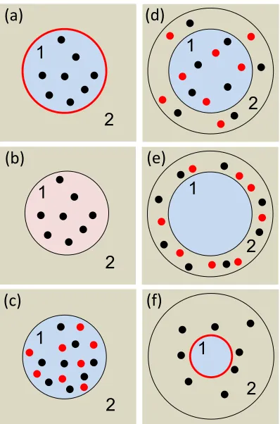
A. Model

Throughout this work, all systems possess a spherical region, which is labeled 1, with a radius

R1, area S1 = 4πR21, volumeV1 = 4πR13/3, and dielectric constant ε1 (see Fig. 2). Region 1 is

immersed in medium 2, which is of infinite extension and has the dielectric constantε2. Hence, whenε2 6=ε1, we have a spherical dielectric discontinuity atR1. Some systems contain a second sphere with radiusR2 > R1, placed concentrically around region 1, and hence sphere 2 divides

medium 2 into two parts. The space between spheres 1 and 2 is referred as to region 2, which consequently has the volumeV2 = 4πR32/3−V1.

all systems and appear as charged hard spheres of radiusRion = 2A and charge˚ q=zione0, where

e0 is the fundamental unit of charge.

Beside mobile ions, some systems also have a stationary charge density. Such a density

gen-erates a potential that acts on the ions, and this potential is referred to as an “external potential”. Two such stationary charge distributions will be employed.

The first one involves an infinite thin shell of a uniform surface charge density σ(r) at the interface between region 1 and 2 and given by

σ(r) = QS S1

δ(r−R1) (21)

where QS is the total charge of the spherical shell. When region 1 is immersed in a continuum medium with the dielectric constant ε2, the electrostatic potential at r generated by the surface charge densityσ(r0)becomes

Z

dr0G0(r,r0)σ(r0) =

QS

ε2R1  



1 forr < R1

R1/r forR1 < r

. (22)

Ions within region 1 experience a constant electrostatic potential from the surface charge density,

regardless of their position within the region. In region 2, ions will experience an electrostatic potential that decays inversely with their distance from the center of region 1.

The second stationary charge distribution is a uniform volume charge densityρ(r)in region 1, given by

ρ(r) = QV V1

 



1 forr < R1

0 forR1 < r

(23)

whereris the distance from the center of region 1, andQV is the total charge of region 1. When

region 1 is immersed in a medium with dielectric constantε2, the electrostatic potential generated atrby the volume charge densityρ(r0)becomes

Z

dr0G0(r,r0)ρ(r0) =

QV

ε1R1      1 2

3− r

2

R2 1

−(1−η) forr < R1

ηR1

r forR1 < r

. (24)

B. Method

Metropolis Monte Carlo (MC) simulations in the canonical ensemble (i.e., at constant number of particles, volume, and temperature) are used to examine the different model systems. The po-tential energy of a system is composed of direct Coulomb and polarization terms. The polarization

energy was evaluated using Eqs. (17), (19), and (20) with the upper infinite limit of their sums overlreplaced bylmax. Moreover, no significant differences were observed betweenlmax = 0and

1(see Sec. IV A 1). Unless otherwise stated, data usinglmax = 0are presented. All energies are

given in kJ (mol ions)−1.

After equilibration, each simulation involved106 _{MC passes (trial moves per ion) for systems}

containing N = 100 counterions and 107 _{MC passes for systems with N < 100. The value of} trial displacements ranged from 2 to 10A. Radial ion density distributions were determined by˚

using a histogram width of0.2_{A. In passing, the statistical uncertainty of the potential energy and}˚ radial density distributions is, for normal requirements, unnecessarily small —104 passes would be sufficient in most cases.

The statistical uncertainties of potential energies were evaluated by repetitively dividing a sim-ulation into blocks of an increasing number of configurations, evaluating the statistical uncertainty

of each block length, and finally extrapolate to infinite block length. This protocol removes the influence of the statistical correlation between successive configuration inherent in the Metropolis Monte Carlo procedure. Uncertainties of radial density distributions were obtained by the simpler

method of divining a run into10subunits that are regarded as statistically independent.

The integrated MC/molecular dynamic/Brownian dynamics simulation package MOLSIM for

molecular systems was employed.16 The inclusion of the polarization energy lengthened the MC simulation times by the factor2.5, as compared to the time where the polarization energy evalua-tion was switched off.

C. Systems

Six types of systems are considered. They differ in terms (i) of the presence of either a

sta-tionary charge distribution or coions to be neutralized by the counterions, and (ii) of the volume available to the ions. Coions and oppositely charged counterions possess the absolute charge

TABLE I. Specification of the types of systems considered, in terms of location of the stationary charge distributions and their counterions, and further specification in terms of the number of ions N, radius of region 1R1, outer radius of region 2R2, and values of the dielectric constants of medium 1ε1, and medium 2ε2.aThe last column indicates the equation used to describe the reformulated Green’s functions.

Type of Location of charges N R1 R2 ε1 ε2 Eq.

system A˚ A˚

A surface charge atS1and counterions inV1 N0 73 ∞ εa εb (17) B volume charge and counterions inV1 N0 73 ∞ εa εb (17) C ions (co- and counterions) inV1 2N0 73 ∞ εa εb (17) D ions (co- and counterions) inV1andV2 2N0 73 92 εa εb (19) E ions (co- and counterions) inV2but outsideV1 2N0 73 92 εb εa (20) F surface charge atS1and counterions inV2but outsideV1 N0 30 92 εb εa (20)

a a_N0 _{∈ {1,5,100},ε}

a ∈ {80,40}, andεb ∈ {80,40,20,10}. Other parameters: absolute ion charge|zion|= 1and temperatureT = 298K.

The six type of systems constitute models for various experimental systems in soft matter such as

microemulsions, micelles, reversed micelles, and cross-liked microgels.

The types of systems are divided into three groups according to the volume available for the

ions. These groups matches the cases presented in Sec. II and are defined as follows:

1. Systems of type A–C comprise counterions confined in region 1, which neutralize (i) in

systems of type A a uniform surface charge distribution at S1, (ii) in systems of type B a uniform volume charge distribution in region 1, and (iii) in systems of type C coions confined in region 1.

2. Systems of type D have the ions confined in regions 1 + 2 withV1 =V2.

3. Systems of type E and F comprise counterions confined in region 2, which neutralize (i) in systems of type E coions confined in region 2 withV2 = V1 and (ii) in systems of type F a

uniform surface charge distribution atS1 withV2 V1.

For each of the six types of systems, we consider throughout three different numbers of

coun-terions N0 combined with eight different choices of (ε1, ε2) – a total of 144 systems. Table I provides a summary of the six types of systems and their specifications including values of N0,

R1,R2,Rion,ε1,ε2, and temperatureT; Fig. 2 displays the types schematically.

respectively. This can be made unambigously for all types of systems except those of type D, where ions appear in both regions – here we let εa denote ε1 and εb denote ε2. The reason for

switching from (ε1,ε2) to (εa,εb) is to achieve a larger degree of similarity of the responses of the systems upon changing the dielectric constants.

IV. NUMERICAL RESULTS AND DISCUSSION

This section is divided into two subsections: the first one contains results on the convergence

of the expansion of the Green’s function and the second one demonstrates effects of the dielectric discontinuities on structural properties. The two subsections are independent of each other and can be read in arbitrary order.

A. Convergence

Numerical results of our simulations are subject to (i) systematic errors arising from the trun-cation of the Green’s function representing energetic contributions from the dielectric

inhomo-geneities given by Eqs. (17), (19), and (20) and (ii) statistical uncertainties due to the finite simu-lation length. Below, we examine how the average potential energy and the radial density distri-butions are affected by these two issues for systems containingN0 = 100counterions. Our focus

will be on the systematic errors, and their magnitudes will be related to the statistical uncertainties.

1. Potential energy

The potential energy among the systems differs strongly, as the electrostatic interaction be-tween counterions and balancing opposing charges is dependent of the volume available to the

counterions as well as of the nature of the balancing charge and its space available. Moreover, the dielectric discontinuity is a source of further variation of the potential energy among the systems.

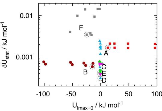
Figure 3 provides an overview of the statistical uncertainty of the potential energy δUstat as a function ofUlmax=0, the latter denoting the average potential energy of the systems obtained with lmax = 0 [i.e., completely omitting the sum over l in Eqs. (17), (19), and (20)]. Data for the

We observe that (i) the potential energy per ion varies from ca. −100 to +100kJ mol−1, (ii) the statistical uncertainty of most systems lies between5×10−4 to10−2kJ mol−1, and (iii) data

of the different types of systems are clustered. In the case of homogeneous dielectric systems, systems of type A and F display the largest magnitude and the largest statistical uncertainty of the potential energy. In systems of type A, the repulsive Coulomb interaction among the

counteri-ons dominates, whereas in systems of type F, the attractive surface charge-counterion interaction dominates. Generally, we see that the statistical uncertainty remains constant or increases with increasing difference of the dielectric constants of the two media. The increase in the statistical

uncertainty is largest for systems of type D, most likely related to the existence of transitions of ions across the dielectric discontinuity.

We will now consider the effect of the truncation of the summation over l in Eqs. (17), (19), and (20). We notice that for ε2/ε1 → ∞, δG0 withlmax = 0 becomes exact. Thus, the infinite

sum only contributes to the difference between the value of ε2/ε1 and ∞(in fact, only a part of it). Initial simulations supported that the convergence of these expansions is very fast, and that it is sufficient to only examine the effect of including the first terml = 1of the infinite sum.

Figure 4 shows |δUl| with δUl ≡ Ulmax=1 −Ulmax=0 denoting the difference in the average

potential energy emerging from simulations with lmax = 1 and lmax = 0 as a function of the

statistical uncertainty of the average potential energyδUstat, obtained withlmax = 0. We observe that the magnitude of the energy differences|δUl|in most cases is smaller or equal to the statistical

uncertainty of the average potential energy δUstat. Considering the length of these simulations providing small values of δUstat, we conclude that the reformulation of the expansion given in Eq. (2) into Eqs. (17), (19), and (20) (i) leads to an expression possessing a very fast convergence

and (ii) the expression ofδG0obtained withlmax = 0is sufficient to achieve an energy convergence of 0.01 kJ mol−1 or better. This holds for an extensive set of different type of systems at various combinations of dielectric constants.

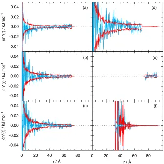
The radial density distributions of mobile ions have been subjected to a similar analysis as the potential energy of the systems. Results of such an analysis applied to systems with the largest

dielectric discontinuity(εa, εb) = (80,10)of each type of system are presented in Fig. 5. In sys-tems containing mobile co- and counterions, where they display same radial density distributions,

type E.

First, we observe that the statistical uncertainty of the reduced radial density distribution

δn∗_stat(r)is largest at the origin and reduces continuously with increasing distance from the origin. This is a direct consequence of the spherical geometry and the use of sampling bins of equal

length. The quantity δn∗_l(r) represents the difference between the radial density distributions obtained from systems with the infinite sums in potential energy terms given in Eqs. (17), (19), and (20) truncated atlmax = 1and0. Second and more importantly, we find|δn∗l(r)| ≤δn

∗ stat(r): the systematic error of truncating the infinite sum isboundedby the statistical uncertainty. Hence, we conclude that in our study the truncation of the infinite sums appearing in the potential energy

expression and arising from the dielectric discontinuity causes a negligible effect on the radial density distributions of the mobile ions.

B. Structural properties

We will here provide radial density distributions of different systems illustrating the effect of a dielectric discontinuity. Such properties of some of the different types of systems have earlier been reported.8,11,12,14 _{Our departure will be homogeneous dielectric systems corresponding to}

water, for which we also will examine the role of different amounts of charge. In the following two subsections, we will present the effects of a dielectric inhomogeneity for the situationsεa> εb andεa< εb, respectively, limited to the largest charge selected andN0 = 100counterions.

In the following, systems of type A–C will be discussed collectively. Whereas the representa-tion of and volume available to the counterions are the same, we recall that these types of systems

differ with respect to the appearance of the other charged species. In systems of type A, this charge is uniformly distributed at the surface of region 1, of type B it is uniformly distributed in the space

of region 1, and of type C it is divided into units carrying one elementary charge and are mobile within region 1 (see Fig. 2a–c). Hence, we can also assess how the different representation of one of the two charged species affects the radial density distribution of the counterions.

1. Dielectric homogeneous systems with different amounts of charge

different amount of charge and number of counterions, viz.N0 = 1,5, and100.

Starting withN0 = 1counterion in the systems of type A, B, and C, we observe in Figs. 6a–c basically uniform counterion distributions. In all three types of systems, the relevant electrostatic

interaction is smaller than the thermal energy and hence too small to significantly affect the prop-erties of the systems. In more detail, in the system of type A the counterion distribution is truly uniform due to a constant external potential, cf. Eq. (22). Furthermore, in the system of type B the

distribution is very weakly shifted toward the center of sphere 1 owing to the radially decreasing magnitude of the attractive external potential, cf. Eq. (24). In the system of type C, no external

potential acts on the ions, nevertheless still a weak depletion of the ions appears near the surface of region 1.

Continuing with systems with increased charge andN0 = 5 and100counterions, the relevant electrostatic interaction will progressively become more important relative to the thermal energy.

The distribution of the counterions in systems of type A is forN0 = 5weakly and forN0 = 100

markedly shifted toward the surface of region 1; in type B forN0 = 5depleted and forN0 = 100

weakly accumulated at the surface of region 1; and in type C remains uniformly distributed but stronger depleted near the surface of region 1.

Thus, systems of type A–C display various responses upon an increase in charge. This variation originates from their different ability of establishing a local screening of ionic charge. In systems

of type A, there is no such screening of the repulsion among the counterions, and their mutual repulsion forces them apart and toward the surface of region 1. In systems of type B with a uniform background charge, there are with N0 > 1 two competing interactions. The mutual

repulsion among the counterions is here counteracted by the the radial potential from the uniform volume charge density. WithN0 = 100the balance has been altered such that the mutual repulsion

among the counterions dominates over the attraction from the volume charge density. In systems of type C, we have a local charge screening among ions of opposite charge, which acts on the length scale of the Debye screening length, here ≈10 ˚A forN0 = 100. Hence, the average ion

density distribution becomes constant with the exception of a depletion near the surface of region 1. This depletion arises from the cohesive nature of the Coulomb interaction due to correlation

effects in combination an anisotropic distribution of surrounding ions of an ion near a surface.

reduced radial density distributions for these three types of systems.

WithN0 = 1counterion, the density distributions in the systems of type D and E are basically

uniform; the depletion effect originating from correlation effects near the dielectric discontinuity is too small to be detected. In the system of type F, a weak accumulation of the counterion at

the charged surface appears. This is the expected outcome, given the attractive potential of the charged inner surface of region 2, cf. Eq. (22).

With increased charge and N0 = 5 and 100 counterions, we observe a depletion of ions at the outer surface of region 2 in the systems of type D and E of the same correlation origin as in systems of type C. In systems of type D, (centers of) counterions are by construction absent in a

shell with width of4_{A. We notice that this gap is too narrow to affect the counterion distribution}˚ near it, whereas for systems of type E a depletion zone appears also at the inner surface of region 2. In the systems of type F, the accumulation of the counterions increases with increasing surface

charge density. At the highest surface charge density andN0 = 100counerions, the contact value atr= 32A amounts to˚ ≈80 and most counterions are located within a shell of10A from the inner˚

surface.

Dielectric homogeneous systems at larger electrostatic coupling than that appearing in aqueous

solutions of monovalent ions, e.g., realized by exchanging monovalent ions to multivalent ones or exchanging water to a solvent with a lower dielectric constant is also of interest. Figure 6 also displays selected reduced radial density distributions obtained at (εa, εb) = (20,20) with N0 =

100 and 50. These systems are trivially equivalent to those specified by (zion, εa, εb) = (2, 80, 80). The system withN0 = 100 is related to the dielectric homogeneous system just discussed by

replacing monovalent ions by divalent ones at constant ion numberdensity and the one with N0

= 50 at constant ioncharge density. For simplicity, these two systems are here referred to ones with divalent ions. Systems of type A, B, and F, remain charge neutral by having the charge of

the counterions and the continuous charge distributions matching each other. In systems of type A and F withN0= 100 (dashed black curves), where all interactions are four-folded increased, we notice that the divalent counterions become more unevenly distributed than in the corresponding

systems with monovalent counterions. The more uneven counterion distribution in system of type A is caused by a stronger counterion–counterion repulsion and in system of type F by a stronger

becomes reduced. This reduced increase is in system of type A caused by the lower counterion number density and in system of type B by the weaker surface–counterion attraction, as compared

to results withN0= 100. Finally, in systems of type B, C, D, and E, the main effect is an enhanced depletion of, now, divalent couterions in the system of type B and of divalent ions in systems of C, D, and E at the uncharged surfaces. The stronger ionic depletion originates from a larger loss

of correlation energy near the surfaces as the cohesive nature of the Coulomb interaction increases with increasing ionic valence.

2. Dielectric inhomogeneous systems: εa > εb

We will now examine the effect of reducing the dielectric constant in the region free of mobil

ions with systems of type D being the only exception. Results will be presented forεa = 80with

εb = 80, 40, 20, and 10 and with N0 = 100 counterions. Table I gives an overview of all the systems investigated.

Figures 7a–c display the evolution of the reduced radial density distributions in systems of

types A–C with decreasing εb. As to systems of type A–C, the major response to the decrease of the dielectric constant in medium 2 located outside medium 1 is a decrease in the counterion density in the vicinity of the dielectric discontinuities, otherwise the radial density distributions

remain basically unaffected. The magnitude of the decrease of the distributions near the surfaces is similar across the three types of systems, and the decease becomes larger as the value of the

dielectric constant in region 2 is decreased.

In systems of type D, a new feature of the ion distribution is shown in Fig. 6d. Here, the ions attain an equilibrium distribution between the two regions of different dielectric constant. To ob-tain a consistent description, an addition of Born1 _{terms have been made to the potential energy}

equations previously given. The Born energy comprises the free energy change of transferring an ion of a certain size from the gas phase to the fluid in question. From these Born energies, the unequal solubility of ions in media of different dielectric constants can be described and

rational-ized; a more negative Born term represents a higher solubility of an ion in a medium with a higher dielectric constant. Figure 7d indeed shows a lowering of the ion density in region 2 upon

the largest dielectric constant.

The systems displaying the weakest response on the reduced dielectric content in region 1 are

of type E (see Fig. 6e). On the level of the uncertainty of the current investigation, the ionic distribution is insensitive to the dielectric constant in region 1. As for the dielectric homogeneous system, at both the inner and outer surfaces of region 2 weak depletions appear.

Finally, we have systems of type F. Briefly, the reduction of the dielectric constant in region 1 reduces the accumulation of counterions at the charged interface as being manifested by a

reduc-tion of the maximum of the density distribureduc-tion. The strength of this addireduc-tional repulsion between a counterion and the dielectric discontinuity depends critically on the distance of the closest

ap-proach between the counterion and the discontinuity. This issues as well as the strong influence of the ionic charge on the repulsion have been subjects of previous studies.8,11,12,14

Hence, in five of the six types of systems, we find in addition to the effect of the Coulomb

interaction that the ion density near the location of the dielectric discontinuities is affected by the discontinuity. The behavior is captured qualitatively by the conventional image charge picture,

which is exact for a planar dielectric discontinuity: an ion experiences a repulsion from (attraction to) a dielectric discontinuity to a medium with a lower (higher) dielectric constant.

3. Dielectric inhomogeneous systems: εa < εb

Systems with dielectric inhomogeneities, where the ions reside in the medium of the lower

dielectric constant, are experimentally difficult to realize. A barrier prohibiting the ions from leaving the medium with the lower dielectric constant and entering the medium with the higher

dielectric constant becomes necessary. We will therefore only compare homogeneous systems with(εa, εb) = (40,80)against inhomogeneous ones having(εa, εb) = (40,80); again withN0 =

100counterions.

In systems of type A–C, Figs. 8a–c shows an enhanced counterion density near the surface of region 1 now surrounded by a region of higher dielectric constant. The spacial range of the

increase is small, only ca. 5_{A. In the systems of type C, closer inspection shows that the radial}˚ density distribution displays a minimum as a consequence of the different length scales of the correlation attraction and the surface polarization interaction.

with Fig. 7d). The same applies to the counterion distribution of the system of type F, cf., Fig. 8f with Fig. 7f. Finally, in the system of type E, the depletion of ions at the surfaces of region 2

increases with the reduction of the dielectric constant of region 2. This is an example of the effect of increased Coulomb coupling. Moreover, the depletion at the two surfaces is unequal. At the inner surface, the depletion due to correlations is partly counteracted by the weaker attraction to

the interface to region 1 with a higher dielectric constant.

V. CONCLUSIONS

We have derived and applied rapidly converged expressions of the Green’s function of the Pois-son equation for symmetric systems with spherical symmetric external potentials including a radial

dielectric discontinuity. These expressions lengthen simulations with a single spherical dielectric discontinuity by only a factor of2.5, as compared to homogeneous dielectric systems. This will facilitate more accurate studies of models of dilute solutions of proteins, surfactant micelles,

col-loidal particles, etc., which generality possess a different dielectric constant as compared to the surrounding solution. The ability to include a single spherical dielectric discontinuity with only a

moderate increase in computational cost makes it promising to simulate solutions of several par-ticles having a dielectric constant different from the solvent. Such simulations restricted to two particles have so far been made17_{to establish two-particle potentials, whereas simulations with a}

larger number of particles are still computationally demanding.

The second outcome of our investigation is an ample number of examples where the compe-tition between the mean-field Coulomb interaction, charge–surface polarization interaction, and correlation effects of the Coulomb interaction is illustrated. The effect of a dielectric discontinuity

on the distribution of ions can conveniently be divided into two parts. First, in the presence of a spatial equilibrium of the ions across the discontinuity, the difference of the density of the ions in the two media is described in the present model by the Born energy. The parameters entering

this expression are the ionic radius and the dielectric constants of the two media. Second, near the dielectric discontinuity, the surface polarization arising from the field of an nearby ion give rise to

ACKNOWLEDGMENTS

Financial support by the Swedish Research Council (VR) through the Linnaeus grant Orga-nizing Molecular Matter (OMM) center of excellence (239-2009-6794) and through individual grants to PL (2010-2253-78321-47) are gratefully acknowledged. Financial support by the

BB-SRC (BB/I017194/1) is gratefully acknowledged by LL.

Appendix A: List of important variables and their symbols

Variable Symbol

number of ions of a givenzion N

volume of region 1 V1

volume of region 2 V2

surface of region 1 and inner surface of region 2 S1

outer surface of region 2 S2

radius of surfaceS1 R1

radius of surfaceS2 R2

relative dielectric constant of medium 1 ε1 relative dielectric constant of medium 2 ε2

radius of an ion Rion

number of elementary charges of an ion zion

temperature T

upper end of summation overlin Eqs. (17)–(20) lmax

Appendix B: Detailed derivations of Eqs.(17),(19), and(20)

Case 1:

If bothrandr0lie inside the sphere, then from Eqs. (3) and (4)

δG0(r,r0) = −

1 ε2ηR

∞ X

l=0

∆(l+ 1) l+ζ t

l_P

l(cosγ) +

η−1−1 ε2|r−r0|

=− ∆

ε2ηR ∞ X

l=0

1 + 1−ζ l+ζ

tlPl(cosγ) +

η−1−1 ε2|r−r0|

=− ∆

ε2ηR

(1−2tcosγ+t2)−1/2− ∆ ε2ηR

∞ X

l=0

1−ζ l+ζt

l

Pl(cosγ) +

η−1−1 ε2|r−r0|

(B1)

wheret =rr0/R2, and we have used the relation18:

∞ X

l=0

tlPl(x) = (1−2xt+t2)−1/2.

If we define the Kelvin point asrK = (R/r0)2r0, then the first term in Eq. (B1) can be rewritten as:

(1−2tcosγ+t2)1/2 = 1 rK

|r−rK|.

The summation in the second term of Eq. (B1) can be rewritten as

∞ X

l=0

tlPl(cosγ)

l+ζ =

∞ X

l=0 Z t

0

dt0t−ζt0l+ζ−1Pl(cosγ)

=

Z t

0

dt01 t0

t0 t

ζ

(1−2t0cosγ+t02)−1/2

=

Z ∞

rK

dxrK x

ζ 1

|r−x|

wherex= (t/t0)rK. Therefore, we can rewrite the polarization contribution to the Green’s

func-tion as

δG0(r,r0) = −

∆ ε2η

rK/R

|r−rK|

− ∆ζη

ε2ηR Z ∞

rK

dxrK x

ζ 1

|r−x| +

The summation in the second term in Eq. (B1) can also be written as

∞ X

l=0

tl_P

l(cosγ)

l+ζ =

∞ X

l=0

1 l+ 1 +

1−ζ (l+ζ)(l+ 1)

tlPl(cosγ)

=−1

t ln

(1−2tcosγ+t2)1/2 −t+ cosγ 1 + cosγ

+η " 1 + ∞ X l=1 ζ

(l+ζ)(l+ 1)t

l_P

l(cosγ)

# (B2)

where we have used the relation18_:

∞ X

l=0

tl_P l(x)

l+ 1 =−

1 t ln

(1−2xt+t2₎1/2_−t+x

1 +x

Substituting Eq. (B2) into Eq. (B1) leads to Eq. (17).

Case 2:

This case is composed of two alternatives. If rlies outside the sphere andr0 lies inside, then

we have

δG0(r,r0) =

1 ε2r

∞ X

l=0

∆l l+ζt

l

Pl(cosγ)

= ∆

ε2r ∞ X

l=0

1− ζ

l+ζ

tlPl(cosγ)

= ∆

ε2r

(1−2tcosγ+t2)−1/2− ∆ζ ε2r

∞ X

l=0

tl_P

l(cosγ)

l+ζ (B3)

wheret =r0/r.

By defining the Kelvin point asrK =r0, we find

(1−2tcosγ+t2)1/2 = 1

The summation in the second term can be recast as an integral:

∞ X

l=0

tl_P

l(cosγ)

l+ζ =

∞ X

l=0 Z t

0

dt0t−ζt0l+ζ−1Pl(cosγ)

= 1 t Z t 0 dt0 t t0 1−ζ

(1−2t0cosγ+t02)−1/2

=

Z rK

0

dxrK x

1−ζ 1

|r−x|

wherex= (t0/t)rK. Substituting these two relations into Eq. (B3), we find Eq. (13).

Equation (19) can be derived for this case by simply substituting Eq. (B2) into Eq. (B3).

Ifrlies inside the sphere andr0lies outside, then

δG0(r,r0) =

∆ ε2r0

(1−2tcosγ+t2)−1/2− ∆ζ ε2r0

∞ X

l=0

tl_P

l(cosγ)

l+ζ (B4)

wheret =r/r0.

Again, defining the Kelvin point asrK =r0, we find

(1−2tcosγ+t2)1/2 = 1

r0|r−rK|.

In an idential manner to the previous case, the summation in the second term in Eq. (B4) can be

rewritten as an integral. Substituting these two relations into Eq. (B3), we find Eq. (9).

Equation (19) can be derived for this case by simply substituting Eq. (B2) into Eq. (B4).

Case 3:

If bothrandr0lie outside the sphere, then we have

δG0(r,r0) =

1 ε2R

∞ X

l=0

∆l l+ζt

l+1

Pl(cosγ)

= ∆t

ε2R ∞ X

l=0

1− ζ

l+ζ

tlPl(cosγ)

= ∆t

ε2R

(1−2tcosγ+t2)−1/2− ∆ζt ε2R

∞ X

l=0

tl_P

l(cosγ)

wheret =R2_/(rr0₎ .

By defining the Kelvin point as rK = (R/r0)2r0, the first term can be rewritten, using the relation

(1−2tcosγ+t2)1/2 = 1

r|r−rK|.

The summation can be converted to an integral as

∞ X

l=0

tlPl(cosγ)

l+ζ =

∞ X

l=0 Z t

0

dt0t−ζt0l+ζ−1Pl(cosγ)

= ∞ X l=0 Z t 0 dt0 t t0 1−ζ

t0lPl(cosγ)

= Z t 0 dt0 t t0 1−ζ

(1−2t0cosγ+t02)−1/2

=

Z rK

0

dxrK x

1−ζ 1

|r−x|

wherex= (t0/t)rK.

Substituting the relation Eq. (B2) into Eq. (B5) leads directly to Eq. (20).

REFERENCES

1_{D. F. Evans and H. Wennerstr¨om,The Colloidal Domain where Physics, Chemistry, Biology, and}

Technology Meet, 2nd ed. (Wiley-VCH, New York, 1999). 2_{R. Messina, J. Phys.; Condens. Matter21, 113102 (2009).}

3_{C. J. F. B¨ottcher,Theory of Electric Polarization, Vol. 1 (Elsevier, Amsterdam, 1973).}

4_{J. D. Jackson,Classical Electrodynamics(Wiley, New York, 1975).} 5_{C. Tanford and J. G. Kirkwood, J. Am. Chem. Soc.79, 5333 (1957).}

6_{G. M. Torrie, J. P. Valleau, and G. N. Patey, J. Chem. Phys.76, 4615 (1982).} 7_{D. Bratko, B. J¨onsson, and H. Wennerstr¨om, Chem. Phys. Letter128, 449 (1986).} 8_{P. Linse, J. Phys. Chem.90, 6821 (1986).}

9_{S. Levine and C. W. Outhwaite, J. Phys. Chem.90, 6821 (1986).} 10_{R. Kjellander and S. Marcelja, Chem. Phys. Lett.142, 485 (1987).} 11_{R. Messina, J. Chem. Phys.117, 11062 (2002).}

13_{I. V. Lindell, Radios Sci.27, 1 (2002).}

14_{L. Lue and P. Linse, J. Chem. Phys.135, 224508 (2011).} 15_{R. A. Curtis and L. Lue, J. Chem. Phys.123, 174702 (2005).} 16_{P. Linse,MOLSIM, Version 5.0, Lund University, Sweden (2011).}

17_{J. Reˇsˇciˇc and P. Linse, J. Chem. Phys.129, 114505 (2008).}

(a)  

r

r´ r_K R

(c)  

r

r´ r_K R

(b)  

r´ r_K

R  

(d)  

r_K r´ R  

(b)  

1

2

(d)  

1

2

(f)  

1

2

(e)  

1

2

(a)  

2

1

(c)  

2

1

-100 -50 0 50 100 0.001

0.01

U_lmax=0 / kJ mol-1

!

Ust

at

/

k

J

m

o

l

-1

A

B C

D F

E

FIG. 3. Statistical uncertainty of the potential energy,δUstat, arising from simulations of finite length, as a function of the potential energy evaluated withlmax = 0,Ulmax=0, in a lin-log scale for systems of type

0.0001 0.001 0.01 0.0001

0.001 0.01

!U_stat / kJ mol-1

|

!

U l

|

/

kJ

mol

-1

FIG. 4. Absolute difference of potential energy,|δUl| ≡ |Ulmax=1−Ulmax=0|, as a function of the statistical

-0.04 -0.02 0.00 0.02 0.04

!

n*(r)

/

kJ

mol

-1

(a)

-0.04 -0.02 0.00 0.02 0.04

!

n*(r)

/

kJ

mol

-1

(b)

0 20 40 60 80

-0.04 -0.02 0.00 0.02 0.04

r / Å

!

n*(r)

/

kJ

mol

-1

(c)

(d)

(e)

0 20 40 60 80

r / Å

(f)

0 1 2 3 4 5 6

n*(r)

8.7

0 1 2

n*(r)

0 20 40 60 80

0 1 2

r / Å

n*(r)

0 20 40 60 80 100

r / Å (a)

(b)

(c)

(d)

(e)

(f)

79.3 210 440

0 1 2 3 4 5 6

n*(r)

0 1 2

n*(r)

0 20 40 60 80

0 1 2

r / Å

n*(r)

0 20 40 60 80 100

r / Å (a)

(b)

(c)

(d)

(e)

(f) _79.3

72.5 66.4 61.6

0 1 2 3 4 5 6

n*(r)

(a)

(b)

(c)

(d)

(e)

(f) 0

1 2

n*(r)

0 20 40 60 80

0 1 2

r / Å

n*(r)

0 20 40 60 80

r / Å 79.3 175