City, University of London Institutional Repository
Citation
:
Bishop, P. G., Bloomfield, R. E., Littlewood, B., Povyakalo, A. A. and Wright, D. (2011). Toward a Formalism for Conservative Claims about the Dependability of Software-Based Systems. IEEE Transactions on Software Engineering, 37(5), pp. 708-717. doi: 10.1109/TSE.2010.67This is the unspecified version of the paper.
This version of the publication may differ from the final published
version.
Permanent repository link:
http://openaccess.city.ac.uk/1070/Link to published version
:
http://dx.doi.org/10.1109/TSE.2010.67Copyright and reuse:
City Research Online aims to make research
outputs of City, University of London available to a wider audience.
Copyright and Moral Rights remain with the author(s) and/or copyright
holders. URLs from City Research Online may be freely distributed and
linked to.
Dependability of Software-based Systems
Peter Bishop, Robin Bloomfield, Bev Littlewood∗, Andrey Povyakalo, David Wright
Centre for Software Reliability, City Unversity, London EC1V 0HB
Abstract
In recent work we have argued for a formal treatment of confidence about the claims made in dependability cases for software-based systems. The key idea underlying this work is ‘the inevitability of uncertainty’: it is rarely possible to assert that a claim about safety or reliability is true with certainty. Much of this uncertainty is epistemic in nature, so it seems inevitable that expert judgment will continue to play an important role in dependability cases. Here we consider a simple case where an expert makes a claim about the probability of failure on demand (pfd) of a sub-system of a wider system, and is able to express his confidence about that claim probabilistically. An important, but difficult, problem then is how such sub-system (claim, confidence) pairs can be propagated through a dependability case for a wider system, of which the sub-systems are components. An informal way forward is to justify, at high confidence, a strong claim, and then conservatively only claim something much weaker: “I’m 99% confident that the pfd is less than 10-5, so it’s reasonable to be 100% confident that it is less than 10-3.”
These conservative pfds of sub-systems can then be propagated simply through the dependability case of the wider system. In this paper we provide formal support for such reasoning.
KEY WORDS: Safety case; system safety; epistemic uncertainty; software reliability; Bayesian probability; confidence measure.
1
Background
There is now a huge literature on the assessment of the dependability of software-based systems, going back several decades. In recent years the assessment process has started to be formalized in dependability cases, most notably safety cases: see, for example (Bishop and Bloomfield 1995; Bloomfield, Bishop et al. 1998; Penny, Eaton et al. 2001; Gorski 2004; Kelly and Weaver 2004). There are now safety standards that require safety cases, e.g. (CAA 2001; MoD 2007)
In this paper we shall discuss some problems arising from the need to assess uncertainty
in cases where dependability claims about a software component form part of a wider
system case. We believe that some aspects of uncertainty have been long neglected or misjudged. For example, expert judgments about the impact of the “quality” of software development processes upon the dependability of software systems often underestimate the uncertainties involved. In recent work we have proposed a formal quantitative
treatment of ‘confidence’ to address this omission (Bloomfield and Littlewood 2003; Bloomfield and Littlewood 2007; Littlewood and Wright 2007).
Computer scientists, including software engineers, have long had an uneasy relationship with uncertainty, and with its most powerful calculus, probability. Some of us can remember discussions of thirty years ago about software reliability. It was difficult then to persuade some software experts that there was inherent uncertainty in the failure processes of programs, and that probability was the appropriate way of capturing this uncertainty. Instead, it was asserted that software failed systematically, and thus that probabilistic notions of ‘reliability’ were meaningless.
Over the years the position has changed. It is now widely agreed that ‘systematic failure’ just means that a program that has failed in certain circumstances will always fail whenever those circumstances are exactly repeated. The uncertainty lies in our not knowing beforehand which circumstances (e.g. inputs to a program) will cause failure, and when these will arise during the operational execution of the program. It is this uncertainty that is represented in a probabilistic measure of dependability, such as probability of failure on demand (pfd).
The uncertainty discussed above concerns system behaviour – it is ‘uncertainty-in-the-world’. In the jargon, this is called aleatory uncertainty. There is another form of uncertainty that has, we believe, been neglected by the software engineering community: this is uncertainty in the dependability assessment process itself. This is called epistemic uncertainty, and it concerns uncertainty in our ‘beliefs-about-the-world’ (Oberkampf and Helton 2004).
The presence of epistemic uncertainty means that we cannot be certain that a claim about dependability – e.g. the pfd is smaller than 10-3
– is true. We might reasonably expect that by collecting more supportive evidence, we would increase our confidence in the truth of the claim, but it will rarely be possible to collect sufficient evidence to eliminate doubt completely.1 This prompts questions such as: How confident are we that the claim is true? How do we express ‘confidence’ quantitatively? How do we incorporate this ‘assessment uncertainty’ into wider dependability cases, and into decision-making?
Consider the simple example of operational testing of an on-demand software-based system. It is put on test and survives 4602 demands without failure. It is a simple statistical exercise (Parnas, Schowan et al. 1990; Littlewood and Wright 1997) to show that you can claim the pfd is smaller than 10-3
with 99% confidence (there is only a 0.01 probability that the pfd is greater than 10-3). The assumptions here include: the oracle is
perfect (i.e. it reports failure if and only if there truly is a failure); the test cases are generated in a way that accurately represents the operational environment (i.e. each is selected with the same probability as in operational use).
If the assumptions are correct in this example, the only epistemic uncertainty arises from the extensiveness of the evidence; if we were to see more failure-free demands, we would have greater than 99% confidence in the claim. When the only epistemic uncertainty is the extensiveness of the evidence, as here, it is easy to compute its impact upon
confidence: for any particular number of failure-free demands it is a simple matter to compute how much confidence we should have in the pfd claim of 10-3
.
In practice, of course, the assessor would not be certain the assumptions were true, and this extra epistemic uncertainty would reduce his confidence in the dependability claim. The impact of assumption doubt upon confidence in a claim is generally harder to quantify, and is likely to involve expert judgment. See (Littlewood and Wright 2007) for a more complex example in which a Bayesian Belief Net is used to structure an argument involving different kinds of assumption doubt. There has been extensive research in recent years on methods for elicitation of expert beliefs to populate such arguments – see (Cooke 2008) for a recent survey – but this remains a difficult area.
The difficulties involved in incorporating software dependability assessment into quantitative safety cases for wider systems, of which the software can be regarded as a component, are well illustrated by the licensing process for the Sizewell B nuclear reactor in the UK in the early 1990s. There was extensive discussion – much of it in the public domain – about the reliability of the software in the primary protection system (PPS). The original reliability requirement for this system was a pfd no worse than 10-4
. However it soon became apparent that nuclear industry experts could not come to a consensus that the evidence (quality of production process, testing and static analysis of the delivered product, etc) was strong enough to support the 10-4
claim with sufficiently high confidence.
The safety system of Sizewell B comprises the software-based PPS and a simpler hardware secondary protection system (SPS) in a 1-out-of-2 architecture (Hunns and Wainwright 1991). When the PPS claim turned out not to be supportable with sufficient confidence, an extensive review of the wider plant safety case was made, including what could be claimed for the SPS. This showed that the contribution of the overall safety system to the plant safety case would be satisfied if 10-3
could be claimed for the PPS (partly because a stronger claim could be made for the SPS).
Using qualitative evidence such as the quality of the production process and extensive static analysis, the regulators accepted that the system was adequately safe based on this revised figure2. Some time later, and following the licensing of the reactor for operation, the PPS software was subjected to extensive statistically representative operational testing. This direct evaluation of its reliability supported the claim of 10-3
pfd at a high confidence level (May, Hughes et al. 1995).
After the licensing of Sizewell B, the UK’s Advisory Committee on the Safety of Nuclear Installations (ACSNI) set up a Study Group on the Safety of Operational Computer Systems, chaired by one of the authors of this paper. Among the recommendations in the final published version of the report (HSE 1998) was the following:
Confidence in assessments of software-based systems is usually less than for more conventionally engineered systems. We believe that attention should be given to incorporating formally in licensees’ and regulatory guidance a
recognition of the importance of the level of confidence that can be placed in assessments of risk within the concept of an ‘adequate’ safety case. What is needed is to clarify and define the notion of ‘adequacy’, such that it can be used to guide and justify decisions as to the required extent of activities that will establish the level of confidence that can be placed in a risk assessment.
During the Study Group’s discussions it was suggested that the UK principle of ALARP (As Low As Reasonably Practicable) – referring to the required safety level (such as pfd) – should be accompanied by a similar one concerning confidence in that level having been achieved: ‘ACARP’ (As Confident As Reasonably Practicable). At the time of writing, this suggestion of a formal demonstration of confidence has not been taken up. However, the experiences from Sizewell and subsequent assessments have been codified in the UK nuclear industry’s reissued Safety Assessment Principles (HSE 2006). These explicitly require confidence building:
361 Independent ‘confidence-building’ should provide an independent and thorough assessment of a safety system’s fitness for purpose. This comprises the following elements:
a) Complete and preferably diverse checking of the finally validated production software by a team that is independent of the systems suppliers, including:
• independent product checking providing a searching analysis of the product;
• independent checking of the design and production process, including activities needed to confirm the realisation of the design intention; and
b) Independent assessment of the test programme, covering the full scope of test activities.
362 Should weaknesses be identified in the production process, compensating measures should be applied to address these. The type of compensating measures will depend on, and should be targeted at, the specific weaknesses found.
The need to address confidence explicitly in the HSE safety assessment principles, and the experience with the discussions about the PPS reliability (where the notion of confidence had been treated rather informally), suggest there may be advantages in exploring more formal – and ideally quantitative – models of confidence. These more formal approaches could provide a semantics for understanding and communicating ‘confidence’, and provide a rigorous framework for negotiation during the licensing process.
An important goal of such a formalism would be to provide a clear notion of how
confident an assessor is, or needs to be. In the Sizewell example there were no clear answers to questions of the following kind:
• How confident was the assessor in the eventually-accepted 10-3
for the pfd of the PPS?
• How confident did the regulator need to be, so as to ‘sign off’ on this part of the safety case?
• How confident was the assessor in the original requirement of 10-4
, and how much did this confidence fall short of what was needed?
In order that an assessor’s epistemic doubt be included in the overall risk assessment, it is necessary that these questions be answered quantitatively in terms of the assessor’s subjective probabilities.
In the Sizewell example, it was also not clear how a pfd level, and the professed confidence in that level, was used:
• If the assessor, or regulator, were ‘sufficiently’ confident in 10-3
, how would this number be used?
• Does ‘sufficiently confident’ mean ‘I can treat the number as if it were true’?
• If, instead, ‘sufficiently confident’ means something like 99% confident, then how is the residual 1% (i.e. the chance that the system is worse than the 10-3
claim) treated?
At one stage there seemed to be reasoning along the following lines: ‘We are reasonably confident that the pfd is better than 10-4
; to be on the safe side, however, we shall only claim 10-3
, and this is so conservative that we can treat this figure as the true pfd in our calculations for the wider system (plant) safety case.’ In this paper we investigate whether this kind of reasoning can ever be justified, and if so whether the resulting numbers can make it a useful approach.
It was interesting in the case of the Sizewell PPS that the numbers involved were rather modest. It seemed possible, in principle, for quite high confidence to be placed in these required levels of reliability. This contrasts with other industries, where the required levels seem so demanding that it will never be feasible to assert high confidence in them convincingly (Butler and Finelli 1993; Littlewood and Strigini 1993). An obvious example concerns the controversial requirement of 10-9
seen. Some railway signaling applications apparently require failure rates no worse than 10-12
per hour (Guiho and Hennebert 1990).
Coming now to a safety case for a wider system – nuclear plant, commercial aircraft type – the top level claim for this system might be expressed, for example, as a probability of (safety-related) failure on demand, or failure rate. This claim will in turn depend upon claims made at lower levels about sub-system functions: e.g. pfd of a protection system, e.g. failure rate of a flight control system. If we knew the values of these sub-system parameters with certainty, then in principle we could decide whether the claim required of the sub-system by the wider safety case had been satisfied. If, on the other hand, these parameters are not known with certainty, as seems likely, then these uncertainties need to be propagated through the safety case, and the reasoning becomes more difficult. In the remainder of the paper it is this problem that we address, when the claims at sub-system level concern software. We are not aware that such problems have been addressed previously in the software engineering literature.
2
Statement of problem, and a conservative solution
As will be clear from the informal discussion above, human judgment inevitably forms an important element of any assessment of confidence (or its complement, doubt) when this arises from epistemic uncertainty. If, as we believe, confidence should be expressed probabilistically, the appropriate calculus of probability is a subjective Bayesian one. The first problem in any Bayesian analysis is to obtain the prior beliefs of the expert. Consider an example in which a pfd is the subject of the dependability claim. This pfd
can be regarded as an unknown number that characterizes the aleatory uncertainty discussed above. In principle, we could estimate this number to any degree of accuracy if we were in the fortunate position of being able to generate unlimited numbers of statistically representative test cases, and we had a perfect oracle to decide whether each test case had been executed correctly. In practice, of course, we are never in this position: instead, there is uncertainty about the value of the pfd. This is the epistemic uncertainty discussed above, arising from imperfect knowledge, etc. This uncertainty about the true value of this pfd requires it to be treated as a random variable, P, so that confidence is expressed as a probability. Thus the expert may believe a priori that
!
Prob(P"y)=1#x (1)
expressing his confidence, 1–x, that the pfd is smaller than y. If the expert were able to tell us the values of x corresponding to all possible values of y, we would have a distribution, say F (with probability density function f), for the random variable P. This would describe the expert’s complete (epistemic) a priori uncertainty about the value of the pfd. In fact it is well-known that experts find it hard to describe their complete uncertainty in this way: it is even hard to elicit just one or two (y, x) pairs.
The second problem concerns how we would use the information even if we knew f
sub-system dependability claims (or dependability claims about many functions) through such complex cases can be difficult or even impossible.
A very informal solution to this problem that we have seen uses the following reasoning: ‘I wish to claim that the pfd of this component (or this function) is better than 10-3
. I will attempt to collect sufficient evidence to be able to make a much stronger claim, e.g. pfd is smaller than 10-5, with high confidence. I will then conclude, because of my high
confidence in this stronger claim, that the weaker claim is conservative (i.e. I am certain that the true pfd is better than this claim). I will then plug this conservative value into my calculation for the overall dependability of the wider system. I am confident that if I do this for all subsystems, my calculated claim for the system will be conservative’
Is such reasoning ever justified? There is an attractive conservatism in the approach. If the evidence is strong enough to replace the numbers in the previous paragraph by ones representing even stronger claims at even higher confidence, surely (it might be reasoned) eventually the expert will allow the modest claim of 10-3
to be treated as if it were true?
In what follows we show that such an approach can be placed on a formal footing. But it turns out that the conservatism in the approach can be very unforgiving, at least until a priori beliefs are supplemented by extensive evidence of failure-free working.
2.1
Result based only on prior beliefs
We start with the very simple situation where the expert has only a priori beliefs about the pfd3. In fact, he is only willing – or able – to express the beliefs represented by (1) above for a single (y, x) pair. In other words, we only know one point on his belief-distribution f.
If we had the complete distribution, then the quantity of interest here is the expert’s subjective probability that there is failure on a randomly chosen demand:
!
Prob(failure on randomly selected demand)= p.f(p)dp
0 1
"
=E(p) (2)by the formula for total probability. This is, for example, the number that the expert might be prepared to ‘plug in’ to a wider safety case: it takes account of the expert’s complete aleatory and epistemic uncertainty.
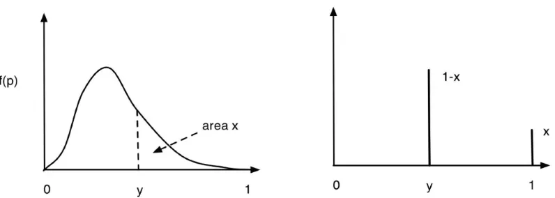
On the left of Figure 1 is a typical distribution for an expert’s belief. In reality, an expert is unlikely to be able to express the infinitely many probabilities implicit in this figure. Instead, he may only be willing to tell us about one point on the distribution: represented here by y. On the right is the most pessimistic of all possible distributions, f(p), that satisfy the expert’s (y,x) belief. It is obtained by placing the probability masses associated
with the intervals (0,y), (y,1) at the extreme right of the intervals. Note that here the bars represent probability mass, in contrast to the probability density function on the left.
Figure 1: A typical distribution for an expert’s belief, and the most pessimistic distribution that satisfies the expert’s (y,x) belief.
The right hand diagram in Fig 1 can easily be seen to represent the ‘most pessimistic’ set of beliefs – i.e. distribution f(p) – that satisfies the expert’s professed belief, (1), because it is the distribution that maximizes (2), giving:
!
Prob(failure on randomly selected demand)= p.f(p)dp
0 1
"
= p.f(p)dp
0
y
"
+ p.f(p)dpy
1
"
<y(1#x)+x=x+y#xy=y*, say.(3)
In other words, if the expert is prepared to accept a claim y with confidence 1-x, as (1) asserts, then (3) shows that he must believe the probability of failure on a randomly selected demand is smaller than y*=x+y-xy. That is, he can treat y* as the true probability of failure on demand – for example in a wider safety case – and be assured that this is a conservative number.
Unfortunately, it is easy to see that this approach is very conservative when only a priori
beliefs are considered, as here. For example, for 10-3
to be an upper bound on the expert’s (subjective) probability of failure on demand, he would need to have 99.91% confidence that the random variable, pfd, is smaller than 10-4
. The problem lies in the exact symmetry of the roles of x and y in (3): any claim, y*, he makes with certainty must be numerically greater than the doubt, x, in the stronger claim, y. Note that this is true regardless of the value of y, but in realistic situations x will usually be much larger than y.
[image:9.612.110.508.140.282.2]2.2
Result based on evidence of failure-free working
It is interesting to ask what is the pessimistic (but attainable) bound for ‘probability of failure on a randomly selected demand’ when some failure-free operation4 has been seen (or, for that matter, some operation that might have included some failures5).
When n failure-free demands have been observed, the expert’s beliefs about P change from his prior belief, represented by f(p), via Bayes theorem: his conditional distribution becomes
!
f(p|n failure - free demands)= (1"p)
n
f(p)dp
(1"p)n f(p)dp
0 1
#
(4)The expert’s posterior probability of failure on demand is just the mean of this:
!
Prob(system fails on randomly selected demand |n failure - free demands) =
!
p
0 1
"
(1#p)n f(p)dp(1#p)n f(p)dp
0 1
"
=E(p|n failure - free demands) (5)
Clearly, the ‘most pessimistic’ 2-point distribution above no longer applies – there cannot be positive probability mass at 1 following the observation of failure-free demands. So the question is: what is the most pessimistic f(p), still satisfying (1), which maximizes (5)?
In fact, somewhat surprisingly, it can be shown that this is once again a 2-point distribution: see Appendix for proof. As before, it has probability mass (1-x) concentrated at y and probability mass x concentrated at z, where the value of z is chosen to maximise the posterior mean of P, which is, by substitution in (5):
!
y(1"y)n(1"x)+z(1"z)nx
(1"y)n(1"x)+(1"z)nx =h(z), say (6) The value of z corresponding to the most pessimistic 2-point (y,z) distribution is the one in (0,1) satisfying h'(z)=0, i.e. satisfying
!
(1"z)n+1x
(n+1)z"ny"1=(1"y) n(1
"x) (7)
for n>0 (for n=0, h'(z)=x>0)
Using this distribution in (5) we obtain the value of the probability of failure on a randomly selected demand that the expert can treat as ‘true’ (e.g. for a wider safety case),
4 Such operation must, of course, be statistically representative of operational use, and the oracle used to determine that all demands are successful must be perfect.
and know that it is conservative (but attainable). It is easy to see from (6) that this ‘true’
[image:11.612.160.458.306.526.2]pfd converges to y as n goes to infinity (with z converging to y), since (1-z)<(1-y).
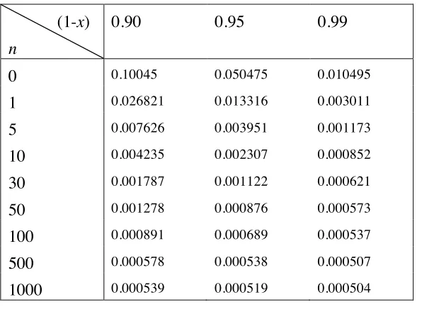
Table 1 shows some examples when the expert expresses his prior beliefs in terms of a claim of 0.5x10⁻³
. Thus when he has a prior confidence of 99% that the pfd is smaller than 0.5x10⁻³
he can only claim 0.010495 with certainty before seeing any evidence of failure-free working. Such unforgiving results from Section 2.1, however, quickly become more useful as evidence of failure-free operation is gathered: with only 50 failure-free demands, and the same prior belief, he can be certain the probability of failure on a randomly chosen demand is better than 0.000573. Compare this with 0.0005 = 0.5x10⁻³
– his original claim in which he had a prior confidence of 0.99. As the evidence of failure-free working gets larger, the expert becomes closer and closer to certain that the original pfd claim is true (a priori, remember, he was only 99% confident in this claim). But the expert can never be certain of a stronger claim that his original 0.5x10⁻³, however much evidence he sees of perfect working.
(1-x)
n
0.90 0.95 0.99
0 0.10045 0.050475 0.010495 1 0.026821 0.013316 0.003011 5 0.007626 0.003951 0.001173 10 0.004235 0.002307 0.000852 30 0.001787 0.001122 0.000621 50 0.001278 0.000876 0.000573
100 0.000891 0.000689 0.000537
500 0.000578 0.000538 0.000507
1000 0.000539 0.000519 0.000504
Table 1. Examples of the worst case true probabilities of failure, based on an expert’s prior beliefs about a claim of y= 0.5 x 10⁻³.
2.3 Result when the expert believes it is possible that there are no faults
A problem with the previous result is that no matter how much evidence of perfect working the expert sees, his worst case probability of failure for a randomly selected demand cannot be better than y: it is easy to see that the expression h(z) in (6) goes to y as
n goes to infinity.
The reason lies in the extreme conservatism of placing all the expert’s belief about the
[image:11.612.162.453.306.519.2]of the mass at z). In the limit all the mass is concentrated at y, but there is still no probability mass to the left of y.
A real expert might regard this result as too conservative: most of us would regard very many failure-free demands to be evidence of very low probability of failure on demand. We might believe that any probability of failure for a randomly selected demand, however small, could be accepted if a sufficiently large number of failure-free demands had been seen.6
As we shall see below, one way this can happen is the situation in which the expert is prepared to believe a priori in the possibility that the system is completely fault-free, however small his prior probability for this.
We proceed by modifying the previous expressions for the expert’s prior beliefs as follows. The expert now believes, before seeing any evidence from the working system:
• Prob(P=0)=α
• For p>0, the expert’s beliefs are represented by an improper probability density function f(p).7 As before he is only willing (or able) to tell us one point on this distribution: Prob(P≤y|P>0)=1-x-α.
This formulation retains the former belief that Prob(P≤y)=1-x, thus allowing a comparison with the earlier results.
The most pessimistic prior satisfying the expert’s beliefs is now the one where (generalizing the right hand distribution in Figure 1) all the probability mass is concentrated at three points:
• Prob(P=0)=α
• Prob(P=y)= 1−x−α
• Prob(P=1)= x
From this pessimistic prior we have:
!
Prob(failure on randomly selected demand)= p.f(p)dp
0 1
"
<x+y#xy#$y=y**
(8)
cf. (3). Once again, the expert can treat y** as the true probability of failure on demand – for example in a wider safety case – and be assured that this is a conservative number. As before, this bound, based solely on prior beliefs, is very conservative, so it is again interesting to see what happens when n failure-free demands have been seen.
The expert’s posterior beliefs are a mixed distribution again, with some probability mass at the origin, and an improper continuous probability density function when p>0:
6 Assuming, of course, that the oracle can be trusted completely, and the operational profile accurately represents real use.
7 That is
!
f(p)dp=1"#
0 1
!
p0(n)"Prob(P=0 |n failure - free demands)=Prob(n failure - free demands and P=0)
Prob(n failure - free demands)
!
= "
(1#p)n f ( p)dp 0
1
$
+"(9)
and
!
f(p|n failure - free demands)= (1"p) n
f(p)
(1"p)n f(p)dp
0 1
#
+$, p>0 (10)
Again this is an improper density function – it does not integrate to unity. Instead
!
f(p|n failure - free demands)dp=1"Prob(P=0 |n failure - free demands) 0
1
#
The expert’s posterior probability of failure on demand is:
!
Prob(system fails on randomly selected demand |n failure - free demands)
!
= p 0 1
"
(1#p)n f ( p)dp(1#p)n f ( p)dp+$ 0
1
"
(11)As before, it can be shown that the most pessimistic improper density, f(p), is a 2-point distribution having probability mass (1-x-α) concentrated at y and probability mass x concentrated at z, where the value of z is chosen to maximise the posterior mean of p, which is, by substitution in (11):
!
y(1"y)n(1
"x"#)+z(1"z)nx
(1"y)n(1"x"#)+(1"z)nx+# (12)
The conservative posterior probability that the system is fault free is obtained by substituting the most pessimistic prior f(p) into the expression (9):
!
p0(n)=
" (1#y)n(1
#x#")+(1#z)nx
+" (13)
It is easy to see that this increases as n increases, and
!
p0(n)"1 as n" #. Thus
As before
!
z"y as n" #. Tables 2, 3 and 4 give some feel for the way in which
posterior beliefs – both for the ‘plug-in’ probability of failure on a randomly selected demand, and for the probability of fault-freeness – depend upon the prior beliefs, and upon the amount of failure-free working that has been seen.
For example, in all cases here the expert will be able to treat the original claim – 0.0005 – as true after only a modest number of failure-free demands. He will be able to treat as true, a claim that is an order of magnitude better than this if he has strong enough a priori
belief in perfection (α=0.9 in Table 3). Whilst such a belief might seem unreasonably strong, it should be remembered that all these results correspond to the same prior belief,
!
Prob(P"y)=1#x: they differ only in how this is partitioned into beliefs about P=0 and 0<P≤y.
(1-x)
n
0.90 Mean
p0(n)
0.95 Mean
p0(n)
0.99 Mean
p0(n)
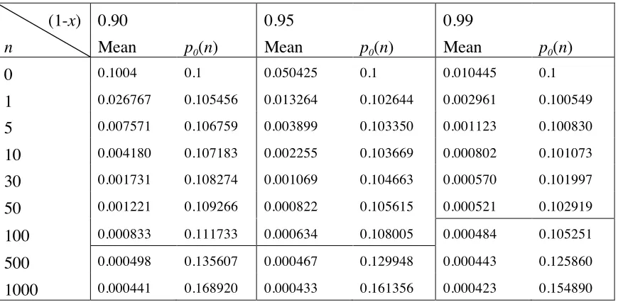
0 0.1004 0.1 0.050425 0.1 0.010445 0.1 1 0.026767 0.105456 0.013264 0.102644 0.002961 0.100549 5 0.007571 0.106759 0.003899 0.103350 0.001123 0.100830 10 0.004180 0.107183 0.002255 0.103669 0.000802 0.101073 30 0.001731 0.108274 0.001069 0.104663 0.000570 0.101997 50 0.001221 0.109266 0.000822 0.105615 0.000521 0.102919 100 0.000833 0.111733 0.000634 0.108005 0.000484 0.105251 500 0.000498 0.135607 0.000467 0.129948 0.000443 0.125860 1000 0.000441 0.168920 0.000433 0.161356 0.000423 0.154890
Table 2 Examples of the worst case true probabilities of failure, based on an expert’s prior beliefs about a claim of y= 0.5 x 10⁻³, with α=0.1. Here, “Mean” is the worst case
probability of failure on demand that the expert can treat as true; “p0(n)” is the expert’s
posterior probability that the system is fault-free. The numbers below the horizontal line in the table correspond to means that are smaller than the original claim of y= 0.5 x 10⁻³,
[image:14.612.91.526.268.481.2](1-x)
n
0.90 Mean
p0(n)
0.95 Mean
p0(n)
0.99 Mean
p0(n)
0 0.1002 0.5 0.050225 0.5 0.010245 0.5
1 0.026550 0.527163 0.013056 0.513111 0.002759 0.502643 5 0.007350 0.533201 0.003689 0.516208 0.000921 0.503638 10 0.003958 0.534725 0.002044 0.517255 0.000599 0.504344
[image:15.612.90.528.71.284.2]30 0.001508 0.537761 0.000858 0.52001 0.000367 0.506893 50 0.000997 0.540268 0.000610 0.522518 0.000318 0.509396 100 0.000607 0.546281 0.000420 0.528668 0.000278 0.515627 500 0.000256 0.605383 0.000238 0.583725 0.000222 0.566232 1000 0.000186 0.667187 0.000189 0.643364 0.000189 0.622626
Table 3. As Table 2, but with α=0.5.
(1-x)
n
0.90 Mean
p0(n)
0.95 Mean
p0(n)
0.99 Mean
p0(n)
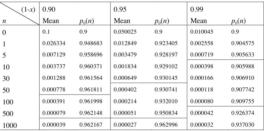
0 0.1 0.9 0.050025 0.9 0.010045 0.9
1 0.026334 0.948683 0.012849 0.923405 0.002558 0.904575 5 0.007129 0.958696 0.003479 0.928197 0.000719 0.905633 10 0.003737 0.960371 0.001834 0.929102 0.000398 0.905988 30 0.001288 0.961564 0.000649 0.930145 0.000166 0.906910 50 0.000778 0.961811 0.000402 0.930741 0.000118 0.907742 100 0.000391 0.961998 0.000214 0.932010 0.000080 0.909755 500 0.000079 0.962148 0.000051 0.950834 0.000042 0.926374 1000 0.000039 0.962167 0.000027 0.962996 0.000032 0.937030
Table 4. As Tables 2, 3, but with α=0.9. Note that the result in the first two columns corresponds to 1-x=α=0.9. In this case the expert’s prior beliefs have no probability density between 0 and y, so the most pessimistic prior has probability mass on only two points, Prob(P=0)=0.9 and Prob(P=1)=0.1, so that the a priori mean is 0.1 as shown in the first cell. The higher horizontal lines here are as in the previous figures. Beneath the lower horizontal lines, the expert can conservatively treat as true a claim that the pfd is no worse than 0.5 x 10⁻⁴, i.e. an order of magnitude better than the original claim (about
[image:15.612.90.524.351.567.2]3
Discussion
We have provided a formalism to support the kind of argument that has sometimes been used informally in real safety cases. That is, an expert can treat a claim about probability of failure on demand as true if he has sufficient confidence – albeit not certainty – in the truth of a stronger claim; and he can be sure that this ‘modest’ claim will be conservative. The value of such an approach, of course, is that this conservative pfd value can simply be ‘plugged in’ to a wider safety case, and the expert can know that the effect on any claims made at this higher level will be conservative.
Not surprisingly, when based upon a priori beliefs alone, such an approach is very
conservative; in fact it is too conservative to have practical usefulness. But when the expert begins to see evidence of failure-free working, this conservatism lessens, and it seems that the results can be useful.
However, as we note, the conservative claim is bounded by the value of y in the expert’s original statement of belief, (y, x). Even with extensive evidence of perfect working, the best that can be claimed is y. It seems reasonable that a real expert would – at least after the fact, when confronted with extensive successful operation – find that this did not represent his expectations. Rather, most experts, we believe, would come to believe that the pfd is smaller than anyy* for sufficiently large n, i.e.
!
y*"0 as
!
n" #.
The reason for the extreme conservatism is that we place all the probability mass lying to the left of y in the expert’s a priori distribution f(p) upon the point y itself. The expert has said initially “all I can tell you about my prior beliefs is that the chance of the pfd being smaller than y is 1-x.” In fact, if specifically questioned about it, it is likely that he would be prepared to say something further along the lines of: “I cannot tell you anything further in detail about how my beliefs are distributed in the interval (0, y), except that f(p) is not zero at any point in this interval.” In other words, our conservatism is too
conservative to represent his beliefs about the pfd in the interval (0, y).
Of course, this extreme conservatism places a serious constraint on the usefulness of the results here. Imagine that, for a wider safety case, we need to claim a pfd no worse than
y* for the system under examination, and that y*<y. No matter how much evidence of successful operation he collects, the expert will not be able to make the y* claim unless he is prepared to expand his expressed a priori beliefs beyond the (y, x) used in our analysis.
Notice how the reasoning required here contrasts with that involved in the analysis of section 2.3. Here the expert believes there is probability mass at the origin, and so is expressing a belief about perfection. He might plausibly reason something like this: “This system has very simple functionality, it has been designed very simply, and I have evidence of certain kinds of formal verification of its correctness, so I think there is a chance that they got it completely right.” This is very different from reasoning that “I know this system is too complex to be correct, so I know it will eventually fail in operation, but I am reasonably confident that the pfd is extremely small.” The two statements are very different in kind, and support for them comes from very different evidence. We think that real experts would be more comfortable with the former than with the latter.
The work reported here represents only the beginnings of a practical probabilistic calculus of confidence for dependability cases – clearly much further work is needed. The problems are both theoretical and practical. Theoretical issues concern the representation and propagation of confidence through complex cases, which typically involve many disparate sources of doubt. Practical issues concern doing this with different, often incomplete, evidence sources.
For example, in this paper we have only considered the situation in which interest centres upon the probability of failure on a randomly selected demand. Imagine, instead, we were interested in the probability of surviving m future demands (say, the number of demands expected in the system’s lifetime). It would be incorrect simply to use the conservative bound, say y*, obtained as above, and estimate this probability using (1-y*)m
. Instead, we would need to find the prior that produces the most conservative value of
!
E((1"P)m).
Similar comments apply to other dependability measures: the point here is that a prior that is conservative for one measure will not generally be conservative for another.
Other issues and questions for future study include the following:
• Does the approach generalize to claims based on continuous measures, e.g. failure rates?
• Can the results be generalized to the multi-attribute case, where claims concern more than one measure, e.g. (pfd, availability)?
• Can other kinds of evidence, of the kinds available for realistic safety cases, be used in this kind of analysis?
Acknowledgement
The work reported here was partially supported by the UK Engineering and Physical Sciences Research Council under the INDEED project.
References
Bloomfield, R. and B. Littlewood (2003). Multi-legged arguments: the impact of diversity upon confidence in dependability arguments. International Conference on Dependable Systems and Networks (DSN2003), San Francisco.
Bloomfield, R. and B. Littlewood (2007). Confidence: its role in dependability cases for risk assessment. International Conference on Dependable Systems and Networks, Edinburgh, IEEE Computer Society.
Bloomfield, R. E., P. G. Bishop, et al. (1998). ASCAD - Adelard Safety Case Development Manual, Adelard.
Butler, R. W. and G. B. Finelli (1993). "The infeasibility of quantifying the reliability of life-critical real-time software." IEEE Trans Software Engineering 19(1): 3-12. CAA (2001). SW01: Regulatory Objective for Software Safety Assurance in Air Traffic
Service Equipment, Civil Aviation Authority.
Cooke, R. M. (2008). "Expert judgement." Reliability Engineering and System Safety (Special Issue) 93(5).
Gorski, J. (2004). Trust Case - A Case for Trustworthiness of IT Infrastructures. NATO Advanced Research Workshop on Cyberspace Security and Defence: Research Issues, Gdansk, Poland.
Guiho, G. and C. Hennebert (1990). SACEM software validation. 12th International Conference on Software Engineering, IEEE Computer Society Press.
HSE (1998). The Use of Computers in Safety-Critical Applications. London, HSE Books. HSE (2006). Safety Assessment Principles for Nuclear Facilities, Health and Safety
Executive, London.
Hunns, D. M. and N. Wainwright (1991). "Software-based protection for Sizewell B: the regulator's perspective." Nuclear Engineering International September: 38-40. IEC (2000). IEC61508: Functional Safety of Electrical, Electronic and Programmable
Electronic Safety Related Systems, Parts 1 to 7, International Electrotechnical Commission.
Kelly, T. P. and R. A. Weaver (2004). The Goal Structuring Notation - A Safety Argument Notation. DSN 2004, Workshop on Assurance Cases.
Littlewood, B. and L. Strigini (1993). "Validation of ultra-high dependability for software-based systems." CACM 36(11): 69-80.
Littlewood, B. and D. Wright (1997). "Some conservative stopping rules for the operational testing of safety-critical software." IEEE Trans Software Engineering 23(11): 673-683.
Littlewood, B. and D. Wright (2007). "The use of multi-legged arguments to increase confidence in safety claims for software-based systems: a study based on a BBN of an idealised example." IEEE Trans Software Engineering 33(5): 347-365. May, J., G. Hughes, et al. (1995). "Reliability estimation from appropriate testing of plant
MoD (1996). Def-Stan 00-56, Issue 2: Hazard Analysis and Safety Classification of the Computer and Programmable Electronic Systems Elements of Defence Equipment, Ministry of Defence.
MoD (2007). Def-Stan 00-56, Issue 4: Safety Management Requirements for Defence Systems, Ministry of Defence.
Oberkampf, W. L. and J. C. Helton (2004). "Alternative representations of epistemic uncertainty." Special Issue: Reliability Engineering and System Safety 85(1-3). Parnas, D. L., A. J. v. Schowan, et al. (1990). "Evaluation of safety-critical software."
Communications ACM 33(6): 636-648.
Penny, J., A. Eaton, et al. (2001). The Practicalities of Goal-Based Regulation. Ninth Safety-Critical Sytems Symposium, Bristol, Springer.
Statement
Let P be the system pfd treated as a random variable with densityf(p). Here we show that
E(P |n failure free demands) = 1−
R1
0(1−p)n+1f(p)dp
R1
0(1−p)nf(p)dp
≤ (1)
1−(1−p1)
n+1(1−x) + (1−p 2)n+1x (1−p1)n(1−x) + (1−p2)nx
where
0≤p1 ≤y≤p2 ≤1
Z y
0
f(p)dp= 1−x.
and the bound (1) is reached with the two-point prior probability distribution of P:
P rob(P =p1) = 1−x; P rob(P =p2) = x;
Lemma
If q is a positive random variable and n is a positive integer, then
[E(qn+1)]n+11 ≥[E(qn)] 1 n
Proof
Ifx≥0 anda≥1 the functionf(x) = xais convex, so, by Jensen’s inequality
E(xa)≥(E(x))a (2)
E(qn+1)≥[E(qn)]n+1n
which implies
[E(qn+1)]n+11 ≥[E(qn)] 1 n
QED
Proof of the statement
Let us introduce four (unknown) values p1, p2, p3, p4
p1 = 1−
Ry
0(1−p)n+1f(p)dp
1−x
!n+11
p2 = 1−
R1
y(1−p)n+1f(p)dp
x
!
1 n+1
p3 = 1−
Ry
0(1−p)
nf(p)dp
1−x
!n1
p4 = 1−
R1
y(1−p)nf(p)dp
x
!
1 n
Obviously,
0≤p1, p3 ≤y
y≤p2, p4 ≤1
In accordance with the lemma
p1 ≤p3 (3)
p2 ≤p4 (4)
because
1−p1 = (E((1−P)n+1 |P ≤y)) 1 n+1
1−p3 = (E((1−P)n |P ≤y)) 1 n
1−p2 = (E((1−P)n+1 |P > y)) 1 n+1
1−p4 = (E((1−P)n |P > y)) 1 n
E(P |n successful runs)
E(P |n successful runs) = 1−
R1
0(1−p)n+1f(p)dp
R1
0(1−p)nf(p)dp
= (5)
1−
Ry
0(1−p)
n+1f(p)dp+R1
y(1−p)
n+1f(p)dp
Ry
0(1−p)nf(p)dp+
R1
y(1−p)nf(p)dp =
1− (1−p1)
n+1(1−x) + (1−p 2)n+1x (1−p3)n(1−x) + (1−p4)nx
Applying (3) and (4) to (5), we finally obtain the following upper bound
E(P |n successful runs)≤1− (1−p1)
n+1(1−x) + (1−p2)n+1x
(1−p1)n(1−x) + (1−p2)nx
(6)
and the bound (6) is obviously reached when one chooses the two-point prior distribution of P:
P rob(P =p1) = 1−x; (7)
P rob(P =p2) = x; 0≤p1 ≤y≤p2 ≤1.
QED
Comment
The unknown values p1 and p2 are found as a solution of two-dimensional
optimisation problem
(1−p1)n+1(1−x) + (1−p2)n+1x (1−p1)n(1−x) + (1−p2)nx
→min (8)
subject to constraints:
0≤p1 ≤y; y≤p2 ≤1.
In general, p1 and p2 may differ from y and 1.