Chaotic duality in string theory

City, University of London Institutional Repository

Citation

:

This is the unspecified version of the paper.

This version of the publication may differ from the final published

version.

Permanent repository link: http://openaccess.city.ac.uk/847/

Link to published version

:

Copyright and reuse:

City Research Online aims to make research

outputs of City, University of London available to a wider audience.

Copyright and Moral Rights remain with the author(s) and/or copyright

holders. URLs from City Research Online may be freely distributed and

linked to.

arXiv:hep-th/0402120v2 27 Apr 2004

Preprint typeset in JHEP style. - HYPER VERSION MIT-CTP-3473 UPR-1065-T NSF-KITP-04-23 hep-th/0402120

Chaotic Duality in String Theory

Sebasti´an Franco1, Yang-Hui He2, Christopher Herzog3 and Johannes Walcher3

1. Center for Theoretical Physics, Massachusetts Institute of Technology Cambridge, MA 02139, USA

2. Department of Physics and Math/Physics RG, The University of Pennsylvania, Philadelphia, PA 19104, USA

3. Kavli Institute for Theoretical Physics, University of California, Santa Barbara, CA 93106, USA

[email protected],[email protected],[email protected],[email protected]

Abstract:_{We investigate the general features of renormalization group flows near superconformal} fixed points of four dimensional N = 1 gauge theories with gravity duals. The gauge theories we study arise as the world-volume theory on a set of D-branes at a Calabi-Yau singularity where a del Pezzo surface shrinks to zero size. Based mainly on field theory analysis, we find evidence that such flows are often chaotic and contain exotic features such as duality walls. For a gauge theory where the del Pezzo is the Hirzebruch zero surface, the dependence of the duality wall height on the couplings at some point in the cascade has a self-similar fractal structure. For a gauge theory dual to P2 _{blown up at a point, we find periodic and quasi-periodic behavior for the gauge theory}

couplings that does not violate thea conjecture. Finally, we construct supergravity duals for these del Pezzos that match our field theory beta functions.

Contents

1. Introduction and Summary 2

2. A Simplicial View of RG Flow 4

2.1 The Klebanov-Strassler Cascade 4

2.2 General RG Flows 6

2.2.1 Beta Functions and Flows 8

2.2.2 Simplices in the Space of Couplings 10

3. Duality Walls for F0 11

3.1 Type A and Type B Cascades 11

3.2 Duality Walls in Type A Cascade 13

3.2.1 Quivers at Step k 13

3.2.2 The RG Flow 15

3.2.3 Duality Walls in Type A Cascades 17

3.3 Fractal Structure of the Duality Wall Curve 17

4. RG Flows and Quasiperiodicity 22

4.1 Initial Theory 22

4.2 RG Flow 23

4.2.1 Poincar´e Orbits 23

4.2.2 Analytical Evolution 25

5. Supergravity Solutions for del Pezzo Flows 28

5.1 Self-Dual (2,1) Solutions 28

5.2 (2,1) Solutions for the del Pezzo 29

5.3 Gauge Couplings 33

5.4 Discussion 35

1. Introduction and Summary

Understanding renormalization group flows out of conformal fixed points of supersymmetric gauge theories is of vital importance in fully grasping the AdS/CFT Correspondence beyond super-conformal theories and brings us closer to realistic gauge theories such as QCD. In particular, the N = 1 gauge theories arising from world-volume theories of D-brane probes on Calabi-Yau singularities have been extensively studied under this light. Dual to these theories are the so-called non-spherical horizons of AdS [1, 2].

A prominent example, the conifold singularity, was analysed by Klebanov and Strassler (KS) in [3] where the RG flow takes the form of a duality cascade. Here, we have a theory with two gauge group factors and four associated bi-fundamental fields. With the addition of appropriate D5-branes, the theory is taken out of conformality in the infra-red. Subsequently, the two gauge couplings evolve according to non-trivial beta functions. Whenever one of the couplings becomes strong, we should perform Seiberg duality to migrate into a regime of weak coupling [3]. And so on do we proceed ad infinitum, generating an intertwining evolution for the couplings. This is called the KS cascade. The dual supergravity (SuGRA) solution, happily aided by our full cognizance of the metric on the conifold, can be studied in detail and matches the field-theory behavior.

One would imagine that a similar analysis, applied to more general Calabi-Yau singularities than the conifold, could be performed, mutatis mutandis. Indeed, a full field theory treatment can be undertaken using various techniques for constructing the gauge theory for D-brane probes on wide classes of singularities. Behavior that differs dramatically from the KS flow has been subsequently observed for, exempli gratia, a class of non-spherical horizons which are U(1) bundles over the del Pezzo surfaces [4, 5]. Using the a-maximization procedures of [6, 7] to determine anomalous dimensions and beta functions, the numerical studies of [5] have convinced us that, sensitive to the type of geometry as well as initial conditions, the quivers after a large number of Seiberg dualities may become hyperbolic in the language of [8]. After this, a finite energy scale is reached beyond which duality cannot proceed. This phenomenon has been dubbed a “duality wall” by [9].

particular, we will formulate the general RG cascade as motion and reflections in certainsimplices in the space of gauge couplings.

Thus girt with the analytic form of the beta functions and Seiberg duality rules [5, 11, 12], we show in Section 3 the existence of the duality wall at finite energy. As an illustrative example, we focus on F0, the zeroth Hirzebruch surface. In the numerical studies of [5], two types of cascading

behavior were noted for F0. Depending on initial values of couplings, one type of cascade readily

caused the quiver to become hyperbolic and hence an exponential growth of the ranks, whereby giving rise to a wall. The other type, though seemingly asymptoting to a wall, was not conclusive from the data. As an application of our analytic methods, we show that duality walls indeed exist for both types and give the position thereof as a function of the initial couplings. These results represent the first example in which the position of a duality wall along with all the dual quivers in the cascade have been analytically determined. Thus, we consider it to be an interesting candidate to attempt the construction of a SuGRA dual. Interestingly, the duality wall height function is piece-wise linear [4, 5] and “fractal.” A highlight of this section will be the demonstration that a fractal behavior is indeed exhibited in such RG cascades. As we zoom in on the wall-position curve, a self-similar pattern of concave and convex cusps emerges.

Inspired by thischaotic behavior, we seek further in our plethora of geometries for signatures of chaos. Moving onto the next simplest horizon, namely that of thedP1, the first del Pezzo surface,

we again study the analytic evolution of the cascade in detail. Here, we find Poincar´e cycles for trajectories of gauge coupling pairs. The shapes of these cycles depend on the initial values of couplings. For some ranges, beautiful elliptical orbits emerge. This type of behavior is reminiscent of the attractors and Russian doll renormalization group flow discussed in [13]. This example constitutes Section 4.

Finally, in Section 5, we move on to the other side of the AdS/CFT Correspondence and attempt to find SuGRA solutions. We rely upon the methodologies of [14] to construct solutions that are analogous to those of Klebanov and Tseytlin (KT) [15] for the conifold. The fact that explicit metrics for cones over del Pezzo surfaces are not yet known is only a minor obstacle. We are able to write down KT-like solutions, complete with the warp factor, as an explicit function of the Cartan matrices of the exceptional algebra associated with the del Pezzo.

We would like to stress the importance of possible corrections to the R-charges of the matter fields, and hence to the anomalous dimensions and beta functions. We will see that in order to be able to follow the RG cascades accurately, we need to be able to assume that the R-charges are corrected only at order_O(M/N)2 _{whereM is the number of D5-branes,N the number of D3-branes,}

and M/N a measure of how close we are to the conformal pointM = 0. In the case of the conifold, the gauge theory possessed a Z_{2 symmetry which forced the O(M/N) corrections to vanish. Our}

del Pezzo gauge theories generally lack such a symmetry.

We have two arguments to address these concerns. First, for KS type cascades, our SuGRA solutions match the field theory beta functions precisely, severely constraining any possible M/N

corrections to the R-charges. For more complicated cascades involving duality walls, we lack SuGRA solutions. Nevertheless, we shall push ahead, assuming that eventually appropriate supergravity solutions will be found and that R-charge corrections, even if_O(M/N), will not change the qualita-tive nature of our results. The flows which we shall soon present are so interesting that we think it worthwhile to describe them in their current, though less than fully understood state. An analogy can be made to the Navier-Stokes equation. Turbulence is observed in fluids in many different situations but is very difficult to model exactly. Instead, people have developed simple models, such as Feigenbaum’s quadratic recursion relation, to understand certain qualitative features, such as period doubling. In some sense, the flows we present here are in relation to the real RG flows as Feigenbaum’s analysis is to the real Navier-Stokes equation.

2. A Simplicial View of RG Flow

In preparation for our discussions on Renormalisation Group (RG) flow in the gauge theory duals to del Pezzo horizons, we initiate our study with an abstract and recollective discussion of RG flows and duality cascades.

2.1 The Klebanov-Strassler Cascade

The Klebanov-Strassler (KS) flow [3] provides our paradigm for an RG cascade. In the KS flow, one starts with an_N = 1 SU(N)_×SU(N+M) gauge theory with bifundamental chiral superfields

Ai and Bi, i = 1,2 and a quartic superpotential. The couplings associated with the two gauge groups we shall respectively call g1 and g2. This quiver theory can be geometrically realized as the

conifold singularity. The matter content and superpotential are given as follows:

B

A

N

N+M

2ǫ

ij_ǫkl_TrA

iBkAjBl . (2.1)

where λ is the superpotential coupling and the trace is taken over color indices.

ForM = 0 the gauge theory is conformal. Indeed, theM D5-branes are added precisely to take us out of this conformal point, inducing a RG flow.

The one loop NSVZ beta function [16] determines the running of the gauge couplings. For each gauge group we have

βi =

d(8π2_/g2

i)

dlnµ =

3T(G)₋P_iT(ri)(1−2γi)

1₋ g2i

8π2T(G)

(2.2)

whereµis a ratio of energy scales and for anSU(Nc) gauge groupT(G) =Nc and T(f und) = 1/2. Using γi = 3₂Ri−1, we can express the beta functions βi=1,2 for the two gauge couplingsgi=1,2

in terms of R-charges. As is done in [3], we will work in the approximation that the denominator of (2.2) is neglected. Then, the beta functions become

β1 = 3 [N + (RA−1)(N +M) + (RB−1)(N+M)] ,

β2 = 3 [(N +M) + (RA−1)N+ (RB−1)N] .

At the conformal point, the R-charges of the bifundamentals can be calculated from the ge-ometry and are RA = RB = 1/2. They can also be simply determined by using the symmetries of the quiver and requesting the vanishing of the beta functions for the gauge and superpotential couplings. Generically, we would expect the R-charges to suffer _O(M/N) corrections for M ₆= 0. Here however, there is a Z_{2 symmetry M → −M for large N that forces the corrections to be of}

order at least O(M/N)2_{. Thus,}

β1 =−3M, β2 = 3M (2.3)

up to O(M/N) corrections.

If we trust these one loop beta functions, then flowing into the IR, we see that the coupling

g2 will eventually diverge because of the positivity of β2. According to Klebanov and Strassler,

the appropriate remedy is a Seiberg duality. After the duality, the gauge group becomes SU(N)_×

x

t

Figure 1: The KS cascade for the conifold. The two inverse gauge couplings x_i=1,2 = _g12 i

for the two nodes evolve in weave pattern against log-energy scale t where Seiberg duality is applied whenever one of the xi’s reaches zero.

sign β1 = 3M and β2 =−3M. This process of Seiberg dualizing and flowing can be continued for

a long time in the large N limit as shown in Figure 1. The number of colors in the gauge groups becomes smaller and smaller. Klebanov and Strassler [3] demonstrated that when one of the gauge groups becomes trivial, the gauge theory undergoes chiral symmetry breaking and confinement. The phenomenon is realized geometrically in the SuGRA dual by a deformation of the conifold in the IR.

Clearly there are some weaknesses in this purely gauge theoretic approach to the RG flow of a strongly coupled gauge theory. Usually Seiberg duality is understood as an IR equivalence of two gauge theories and is not performed in the limit g2 → ∞. Can we really trust Seiberg duality here?

Also, we have dropped the denominator of the full NSVZ beta function (2.2), which is presumably important. Nevertheless, the analysis is sound and the strongest argument for the validity of these Seiberg dualities comes not from gauge theory but from the dual supergravity theory [3]. There is a completely well-behaved supergravity solution, the KS solution of the conifold, which models this RG flow. On the gravity side, there is a radial dependence of the 5-form flux which produces a logarithmic running of the effective number of D3-branes in complete accordance with the field theory cascade, giving credence to these Seiberg dualities.

2.2 General RG Flows

17, 18, 19, 20] for a comprehensive discussion). With some important caveats, these theories can be treated in a fashion similar to the discussion above for the conifold.

The field content of a del Pezzo gauge theory is described compactly by a quiver. For D-branes probing the n-th del Pezzo, the number of gauge group factors in the quiver theory is equal to

k=n+ 3 , (2.4)

which is the Euler characteristic χ(dPn). We reserve the index i= 1,2, . . . k for labeling the nodes of the quiver. We denote the adjacency matrix of the quiver by fij. In other words, fij is the number of arrows in the quiver from node i to nodej. We point out that by definition, thefij are all non-negative.

Thus given a quiver, we need to specify the ranks of the gauge groups in order to define a gauge theory. We will denote the rank of the gauge group on the i-th node by di_{, and the dimension} vector by d= (di₎

i=1,...,k. As on the conifold, the ranks di are related to the number of branes that realize the specific gauge theory in string theory. When probing the del Pezzos, we will reserve N to denote the number of regular D3-branes, andMI _{to denote the number of D5-branes. The D3-brane} corresponds to a unique dimension vector which we will denote by r = (ri₎

i=1,...k. In distinction to the conifold and its ADE generalizations, the possible D5-branes are constrained by chiral anomaly cancellation, and we will parametrize their dimension vectors by sI = (siI) with I = 1,2. . . , n.

Summarizing, a D-brane configuration withN regular D3-branes and MI _{D5-branes of type I}

corresponds to the gauge group Qk i=1

SU(di_{) with}

di =riN +si_IMI (2.5)

and fij chiral fields Xij in the SU(di)×SU(dj) bi-fundamental representation.

As shown in [11, 12], the beta functions of the gauge theory can be computed effectively from geometry by taking advantage of the exceptional collection language [10, 11, 12, 21]. An exceptional collection E = (E1, E2, . . . , Ek) is an ordered collection of sheaves, specifying the D-brane associated with each node. The intersections of the sheaves give rise to massless strings which in turn correspond to bifundamental fields in the gauge theory. E can roughly be thought of as a basis of branes.

If a given quiver satisfies the well split condition of [11], the order of the quiver changes in a simple way under Seiberg duality. To understand the well split condition, we first need to refine our understanding of the quiver ordering. It was shown in [11] that the ordering of the quiver is only determined up to cyclic permutations. If 123. . . n is a good ordering, then so is 23. . . n1. If a quiver is well split, then we can find a cyclic permutation such that for any node j, all the outgoing arrows from j go to nodes i < j and all the in-going arrows into j come from nodes i > j. After a Seiberg duality on node j,j would become the last node in the quiver.

An unproven conjecture of [11] is that the Seiberg dual of a well split quiver is again well split. The conjecture was proven for four node quivers in [11] and no counter-examples are known to the authors. An appropriate understanding of ill split quivers is still lacking. For example, the correct determination of R-charges for them is still open [11]. Indeed, the fractional Seiberg dualities encountered in [21] may be problematic precisely for this reason. As our examples in the subsequent sections involve only Seiberg dualities of well split, four node quivers, we can be confident in our calculations.

In light of the exceptional collection language, we shall also make use of the matrixS which is an upper triangular matrix with ones along the diagonal and related to fij by

Sij =

      

fij −fji , i < j ;

1 , i=j ;

0 , i > j .

, (2.6)

where we have assumed an ordering. The componentsSij,i6=j, are still the number of arrows from node i to node j, except that now a negative entry corresponds to reversing the arrow direction. We will find it convenient to use a matrix _I which is simply the antisymmetrized version of S (or

f).

I =S−St =f −ft (2.7)

Using this, chiral anomaly cancellation can be concisely expressed as the condition that the dimen-sion vector d be in the kernel of_I. In other words, r and the sI form a basis of kerI.

2.2.1 Beta Functions and Flows

the bifundamental Xij, one obtains for the beta function of the i-th node (cf. Eq (5.7) of [5])

dxi

dlnµ =βi = 3d

i₊3 2

k

X

j=1

(fij(Rij −1) +fji(Rji−1))dj

!

. (2.8)

where xi is related to thei-th gauge coupling via xi ≡8π2/gi2.

One very insightful approach for the determination of the R-charge is the procedure of maxi-mization of the central chargea in the CFT as advocated in [6, 7]. We shall however adhere to the procedure of [11, 12], which gives the R-charges at the conformal point. Transcribing Eq. 49 from [12] to present notations, the R-charge of the bi-fundamental Xij is given by

R(Xij) = 1 +

2

(9₋n)ri_rj(S

−1

ij +S

−1

ji )−1

sign(i−j) . (2.9)

It was shown in [12] that plugging (2.9) into (2.8), and going to the conformal point di _{= r}i_{, one} finds βi = 0, as expected.

The flow is induced when we leave the conformal fixed point by adding D5-branes. As in [3], we will work in the regime MI _{≪ N. We will assume the R-charges do not receive corrections of}

O(MI_{/N). This assumption is supported by the supergravity solutions we write down in section} 5, which severely constrain the nature of such corrections for KS type cascades. For more general cascades with duality walls, we believe that we can still trust the qualitative nature of our results. Ignoring the corrections, the non-conformal beta functions can readily be obtained by substituting (2.9) into (2.8) for general ranks di_{. We obtain, to order M}I_/N,

βi = 3siIMI +

3 2

X

j

e

RijsjIMI, (2.10)

where we have introduced the symmetric matrix

e

Rij =fij(Rij −1) +fji(Rji−1). (2.11)

We will now evolve the inverse gauge couplings xi = 8π2/g2i with the beta functions (2.10). Since the one-loop beta functions are constant, the evolution proceeds in step-wise linear fashion, much like the KS cascade; we have

8π2

g2

i(t+ ∆t)

− 8π

2

g2

i(t)

=βi∆t (2.12)

An important constraint can be placed on this evolution. Even though now these beta functions do not vanish identically, it is still the case that

k

X

i

βiri = 0. (2.13)

The reason is that this sum can be reorganized into a sum over each of the beta functions at the conformal point, and at the conformal point, each of these beta functions vanishes individually. It follows from (2.10) and (2.13) therefore, that,

k

X

i

ri

g2

i

= constant (2.14)

throughout the course of the cascade; on this constraint we shall expound next.

2.2.2 Simplices in the Space of Couplings

The space of possible gauge coupling constantsxi ≡1/g2i for a quiver withk gauge groups is a cone (R₊₎k_{. The relation (2.14) cuts out asimplexin this cone. The beta functions (2.10) establish the}

direction of the renormalization group flow inside this simplex. For the KS conifold flow, having two gauge couplings, the cone is the quadrant in R2 _{parametrized by 1/g}2

1 =x > 0 and 1/g22 =y >0.

The simplex is the line segment x+y= const inside this cone. The beta functions tell us to move up and down this line segment until one or the other coupling constant diverges.

In more general cases, under the renormalization group flow, we will eventually reach a face of the simplex where one of the couplings diverges. At this point, the insight gained from the KS flow tells us we should Seiberg dualize the corresponding gauge group. After the duality, we find ourselves typically in a new gauge theory. The new gauge theory has some new associated simplex and renormalization group flow direction given by some different set of beta functions. The KS flow is very special in that the Seiberg dual theory is identical to the original one up to the total number of D3-branes N.

One imagines in general some huge collection of simplices glued together along their faces. In any given simplex, the renormalization group trajectory is a straight line. At the faces, the trajectory “refracts”. One recomputes the beta functions to find the new direction for the RG flow. In Figure 1 for example, we have the evolution of the couplings reflecting off thet-axis (corresponding to either 1/g2

1 or 1/g22 equal to zero), whereby giving the weave pattern. Note that such RG flows

the trajectory such that a different face of a simplex is reached. A different face corresponds to a Seiberg duality on a different node which will generically completely alter the rest of the flow. Such a sensitivity was noticed in [4, 5].

For four node quivers, the simplices are tetrahedra and the RG flow can be visualized. There is only one vector s, with components si, corresponding to only one D5-brane. Thus, the direction of the RG flow inside any given tetrahedron is, up to sign, independent of M. Moreover, one can show that after a duality on node i, βi → −βi (see the appendix for details).

Thus prepared, we can embark upon a detailed study of the RG flows and duality cascades for various concrete examples. Some of them will exhibit a KS type behavior, meaning that the cascade will periodically return to the same quiver up to a change in the number of D3-branes, showing no accumulation of dualization scales in the UV. Others will be markedly different, exhibiting duality walls. In particular, we shall describe an assortment of interesting flows for D-branes probing cones over the del Pezzo surfaces, where we will be able, in addition to numerics, to gain some quantitative analytic understanding.

3. Duality Walls for

F

We begin with D-brane probe theories on the complex cone over F0, the zeroth Hirzebruch surface.

The addition of D5-branes takes us out of conformality, whereby inducing a RG flow. Detailed numerical study was undertaken in [5]. All Seiberg dual theories for this geometry can be arranged into a web which encodes all possible duality cascades. This web takes the form of a flower and has been affectionately called the Flos Hirzebruchiensis (cf. Fig 7 cit. Ibid.). The purpose of this section is to derive analytical results for the existence of duality walls and their location. We also explain the fractal structure of the duality wall curve as a function of the initial couplings.

3.1 Type A and Type B Cascades

Before proceeding with the analytical derivations, let us make a brief summary of the findings in [5], where two classes of RG trajectories were identified. In one gauge theory realization, F0 exhibits a

Klebanov-Strassler type flow that alternates between two quivers with constant intervals int= logµ

>> >> >> >> 1 2 3 4 >> >> >> >> >>>> 1 2 3 4 N N+M N+M N N N+M N+M N+2M

β = −3Μ

β = 3Μ

3

β = 3Μ

β = −3Μ

β = −3Μ

β = 0

3

β = 0

β = 3Μ

Figure 2: The first class of duality cascades for F0. This is an immediate generalization of the KS conifold

case and we alternate between the two theories upon dualizing node 3 of each and evolve according to the beta functions shown. 3N N-M N+M N 1 2 3 4 > >

> _> >

2

4

6 2

6

β = 0

β = −3Μ

3

β = 3Μ

β = 0

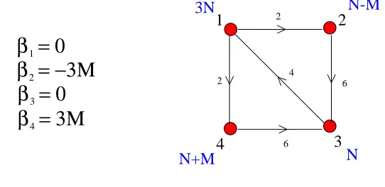
Figure 3: The second class of theories for F0. Starting from this quiver and following the duality cascade

give markedly different behavior from the KS case. It was seen in this case that the increment in energy scale decreases at each step and a “duality wall” may be reached [5].

The second class of flows commences with the quiver in Figure 3, which is another theory in the duality flower for F0. In this case, there is a decrease in the t interval between consecutive

dualizations towards the UV, leading to the possibility of a so-called “duality wall” past which no more dualization is possible and we have an accumulation point at finite energy. Considering initial couplings of the four gauge group factors of the form (1, x2, x3,0), two qualitatively different

behaviors were observed.

1. In theories withx3 >0.9, the cascade corresponds to an infinite set of alternate dualizations of

that in this case a duality wall is indeed approached smoothly.

2. On the other hand, for x3 < 0.9, the third gauge group is dualized at a finite scale. When

this happens, all the intersection numbers in the quiver become larger than 2, leading to an explosive growth of the ranks of the gauge groups and the number of bifundamental chiral fields, and generating an immediate accumulation of the dualization scales. This discontinuous behavior makes duality walls evident even in numerical simulations for these flows. We will refer to these flows as B type cascades.

3.2 Duality Walls in Type A Cascade

Having elucidated the rudiments of the cascading behavior of theF0 theories, let us explore whether

there are indeed duality walls for A type cascades, which we recall to be the type for which numeri-cal evidence is not conclusive. We shall proceed analytinumeri-cally. In order to do so, let us first construct the quiver at an arbitrary step k. We can regard Seiberg duality as a matrix transformation on the rank vector and the adjacency matrix as was done for example in Sec. 8.1 of [5]. An elegant way to derive the quiver at a generic position in the cascade is by realizing Seiberg duality trans-formations as mutations in an exceptional collection (equivalently, by Picard-Lefschetz monodromy transformations on the 3-cycles in the manifold mirror to the original Calabi-Yau). We will use this language as was done in [11, 12].

Taking the exceptional collection to be (a, b,3,4), the alternate dualizations of nodes 1 and 2 corresponds in this language to the repeated left mutation of a with respect to b. For even k

(a, b) = (1,2), while for odd k (a, b) = (2,1). Figure 3 corresponds to k = 1 where the exceptional collection ordering is (2,1,3,4). This quiver is well split.

3.2.1 Quivers at Step k

Under Seiberg duality, the rank of the relevant gauge group changes from Nc to Nf −Nc. Type A cascades correspond to always dualizing node a. By explicitly constructing these RG trajectories, we will check that this assumption is indeed consistent. The exceptional collection tells us that after the duality, nodes a and b will switch places. Thus

Na(k+ 1) =Nb(k) ,

Nb(k+ 1) = 2Nb(k)−Na(k) .

6 2

2(k−2)

2(k−1)

2(k+2)

2(k+1)

N

N

N

N

Figure 4: Quiver diagram at stepkof a type A cascade for F₀.

It is immediate to prove that after k iterations, the ranks of theSU(Ni) gauge groups are given by

Na = (2k−1)N+ (k−2)M ,

Nb = (2k+ 1)N + (k−1)M ,

N3 =N ,

N4 =N +M .

(3.2)

The number of bifundamental fields between each pair of nodes follow from applying the usual rules for Seiberg duality of a quiver theory. In particular, we combine the bifundamentals Xa4, Xba, and

Xa3 into mesonic operators Mb4 = XbaXa4 and Mb3 = XbaXa3. We introduce new bifundamentals

X′

4a, X

′

ab, andX

′

3awith dual quantum numbers along with the extra termMb4X4′aX

′

ab+Mb3X3′aX

′

ab to the superpotential. We then use the superpotential to integrate out the massive fields, which appear in the quiver as bidirectional arrows between the pairs of nodes (3, b) and (4, b). The resulting incidence matrix for the quiver will change such that

fba(k+ 1) =fba(k) f3b(k+ 1) =fa3(k) f43(k+ 1) =f43(k)

fa4(k+ 1) =−f4b(k) + 2fa4(k) f4b(k+ 1) =fa4(k) fa3(k+ 1) =−f3b(k) + 2fa3(k)

(3.3) which can be simplified to yield

fba(k) = 2 f3b(k) = 2(k+ 1) f43(k) = 6

fa4(k) = 2(k−1) f4b(k) = 2(k−2) fa3(k) = 2(k+ 2) .

(3.4)

With the adjacency matrix (3.4) and the non-conformal ranks (3.2), we can readily compute the beta functions from (2.10), to arrive at

βa =−9(₍₄k+1)_k+2)kM <0

βb = 9(k

−_1)kM

(4k−2) ≥0

β3 = 3(7k

2_−3k−4)M

(2−8k2₎ <0

β4 = 3(7k

2_+3k−4)M

(−2+8k2₎ >0,

k = 1,2,3, . . .

(a, b) = (2,1); k odd (a, b) = (1,2); k even

(3.5)

3.2.2 The RG Flow

Using the results in Section 3.2.1, we proceed to study the evolution of the dualization scales starting with the initial couplings (1, x2(0), x3(0),0). Let us consider the first step in the cascade. We are

in a type A cascade, so x3(0)>0.9. The beta functions are, from (3.5),

β1(1) = 0, β2(1) =−3M, β3(1) = 0, β4(1) = 3M . (3.6)

We see that only node 2 has a negative beta function at the first step and so its associated coupling will reach zero first, i.e., the first step ends with the dualization of node 2. The subsequent increment ∆(1) in the energy scale t= logµbefore the dualization is performed is equal to

∆(1) = x2(0) |β2(1)|

. (3.7)

Applying

xi(k+ 1) =xi(k) +βi(k+ 1)∆(k+ 1), t(k+ 1) =t(k) + ∆(k) , (3.8)

we have at the end of this step

x1(1) = 1, x2(1) = 0, x3(1) =x3(0), x4(1) =

3Mx2(0)

|β2(1)|

. (3.9)

So, as far as nodes 2 and 3 are concerned, the initial value x2(0) only affects the length of the first

step, beyond which any information about it is erased. In order to look for the initial couplings that lead to a type A flow, recall that we have to determine the possible initial values x3(0) such that x3(k) remains greater than zero as k → ∞ so that the third node never becomes dualized. Since β3(1) = 0, this is completely independent of ∆(1) and hence independent of x2(0).

That said, let us look at the cascade at the next step. The beta functions (3.5) now give

β1(2) =−

27

5 M, β2(2) = 3M, β3(2) =− 9

Since we are interested in type A cascades, we assume that the initial value x3(0) is such that this

node is never dualized. Thus, the next node to undergo Seiberg duality is the other one with a negative beta function, namely node 1. Recalling thatx1(1) = 1, the consequent step in the energy

scale ∆(2) is thus

∆(2) = x1(1) |β1(2)|

= 1

|β1(2)|

, (3.11)

and x1(2) = 0 while x2(2) =β2(2)∆(2). Proceeding similarly, the next step gives

∆(3) = β2(2)

β1(2)

1

β2(3)

. (3.12)

We see that in general, at the kth _{step, the interval ∆(k) is given by}

∆(k) =

" _k Y

i=2

βb(i)

|βa(i)|

#

1

βb(k)

, (a, b) = (2,1), k odd;

(a, b) = (1,2), k even , (3.13)

for k _≥2. This, using (3.5), can be written as a telescoping product

M∆(k) =

" _k Y

i=2

(i−1) (i+ 1)

(2i+ 1) (2i₋1)

#

(4k−2)

9(k₋1)k . (3.14)

Simplifying this expression we arrive at

M∆(k) = 2(2k+ 1)(4k−2)

27k2_(k2 ₋₁₎ (3.15)

for k _≥2. The total variation of the third coupling x3, after k steps, is given by

x3(k)−x3(0) =

k

X

i=2

∆(i)β3(i) . (3.16)

As discussed, the boundary between type A and B cascades corresponds to initial conditions such thatx3(k)→0 fork → ∞, i.e., the initial conditions that separate the regime in which node 3 gets

dualized at some finite k from the one in which it never undergoes a Seiberg duality. Then,

x3(0)−x3(∞) =

2 9

∞

X

i=2

(7i+ 4)

i2_{(i+ 1)} =

4 27π

2

− 5

9 . (3.17)

3.2.3 Duality Walls in Type A Cascades

The computations in the previous section enable us to address one of the questions left open in [5], namely whether duality walls exist in this case. Our flow, from (3.17), corresponds to an infinite cascade that only involves nodes 1 and 2. Let us sum up all the steps ∆(k) in the energy scale ad infinitum; this is equal to

∞

X

k=1

∆(k) = ∆(1) +

∞

X

k=2

∆(k) . (3.18)

Using ∆(1) =x2(0)/|β2(1)|=x2(0)/3M and (3.15), we see that this sum can actually be performed,

giving us a finite answer. This means that there is indeed a duality wall for our type A cascades, whose value is equal to

twall =

1 3M

x2(0) +

2π2

27 + 5 9

. (3.19)

We would like to emphasize that, although derived in the approximation of vanishing O(M/N) corrections to the R-charges, (3.19) is the first analytical result for a duality wall. Given the detailed understanding we have of every step of the cascade on the gauge theory side, this example stands as a natural candidate in which to try to look for a realization of this phenomenon in a SuGRA dual.

3.3 Fractal Structure of the Duality Wall Curve

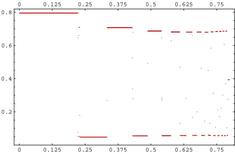
Having analytically ascertained the existence and precise position of the duality wall for type A cascades, and the boundary value x3b(0) of the inverse squared coupling at which the cascades become type B, we now move on to address another fascinating question, hints of which were raised in [5, 12], viz., the dependence of the position of the wall upon the initial couplings. We will see that, in type B cascades, such dependence takes the form of a self-similarcurve.

Let us focus on the one dimensional subset of the possible initial conditions given by couplings of the form (1,1, x3(0),0) (more general initial conditions can be studied in a similar fashion).

Figure 5 is a plot of the position of the duality wall as a function ofx3(0). Initial valuesx3(0)> x3b correspond to type A cascades. Node 3 is not dualized in this case and thus the position of the wall is independent of x3(0) in this range, as determined by (3.19). From now on, we will focus on the

x3(0)< x3b type B region. The curve exhibits in this region an apparent piecewise linear structure

as was noticed in [5].

0 0.125 0.25 0.375 0.5 0.625 0.75 0.4

0.5 0.6 0.7

0 0.125 0.25 0.375 0.5 0.625 0.75

Convex

Concave

Figure 5: Position of the duality wall for F0 as a function of x3(0) for initial conditions of the form

(1,1, x3(0),0). A piecewise linear structure is seen for the type B cascade region, i.e., x3(0)< x3b ∼0.9.

0 0.125 0.25 0.375 0.5 0.625 0.75

0.2 0.4 0.6 0.8

0 0.125 0.25 0.375 0.5 0.625 0.75

Figure 6: Derivative of the position of the duality wall forF0 as a function ofx3(0)for initial conditions of the

form (1,1, x3(0),0). The appearance of the constant segments evidences further the piecewise linear behavior

of position of the wall with respect to x₃(0).

in fact approximate, and an intricate structure is revealed when we look at the curve in more detail. While exploring the origin of the different features of the curve, we will discover that a self-similar fractal structure emerges.

the one at ≃0.3 is a concave one. We will explain now their origin and give analytical expressions for their positions.

As we will illustrate with examples, this kind of structure appears at those values of the couplings at which a transition between different cascades occurs. A semi-quantitave measure of how different two cascades are is given by the number of steps m that they share in common. In this sense, if a given cascade A shares m1 steps with cascade B and m2 with cascade C, with m1 > m2, we say

that A is closer to B than to C. The general principle is that the closer the cascades between which a transition occurs at a given initial coupling, the smaller the corresponding feature in the position of duality wall versus coupling curve is.

It is important to remember what the physical meaning of our computations is. Numbering cascade steps increasing towards the UV and identifying the values of the initial couplings are just a simple way to handle the process of reconstructing a duality cascade. This cascade represents a traditional RG flow in the IR direction, in which Seiberg duality is used to switch to alternative descriptions of the theory beyond infinite coupling. At some stage of this flow in the IR the model in Figure 3 appears, with couplings given precisely by what we called initial conditions. Thus, two cascades that share a large number of steps m in common, correspond to two RG flows initiated at different theories with large gauge groups and number of bifundamental fields in the UV that converge at some point, sharing the last m steps prior to reaching the model in Figure 3. Due to the fact that a duality wall exists, the independent flows before convergence of the cascades take place in a very small range of energies.

We now investigate the convex and concave cusps of the curve. Our approach consists of identi-fying what happens to the cascades at those special points, and then computing the corresponding values of the initial couplings analytically. Let us first consider theconcave cusps. Them-th concave cusp corresponds to the transition from node 3 being dualized at step m+ 1 to it being dualized at step m+ 2. The cascades at both sides of the m-th concave cusp share the firstm steps and are of the form

2121. . . a3

2121. . . a

| {z }

m

b3 (3.20)

and (3.17) for k≥2, i.e.

xconc₃ (k) = 2

9 k

X

i=2

(7i+ 4)

i2_{(i+ 1)} k ≥2. (3.21)

From (3.21), the first concave cusps are located at x3(0) equal to

1 3, 79 162, 467 810, 2569 4050, 19133

28350 , . . . (3.22)

in complete agreement with the numerical values of Figures 5 and 6.

Let us move on and study the convex cusps in Figure 5. In analogy with (3.20), we claim that the mth convex cusp corresponds to cascades switching between

2121. . . a3a

2121. . . a

| {z }

m

3b (3.23)

with (a, b) = (1,2) form even and (2,1) form odd. In order to check whether the proposal in (3.23) is correct, we proceed to compute the positions for the cusps that it predicts. The calculation is similar to the one in _§ 3.2.2 and we only quote its result here

xconv

3 (k) =

(4 + 7k)(10 + 49k+ 50k2_{+ 14k}3₎

9k2_{(1 +k)}2_{(3 + 22k+ 14k}2₎ +

2 9

k−1 X

i=2

(7i+ 4)

i2_{(i+ 1)} , k ≥2 . (3.24)

Equation (3.21) determines the following positions for the first convex cusps

70 309, 21773 50544, 76733 141750, 457831 750060, 83386559

126809550 , . . . (3.25)

which are in perfect accordance with Figures 5 and 6, whereby validating (3.23).

The Fractal: Something fascinating happens when the duality wall curve is studied in further detail. Although convex cusps appear as such when looking at the curve at a relatively small resolution as in Figure 5, an infinite fractal series of concave and convex cusps blossoms when we zoom in further and further. As an example, we show in Figure 7 successive amplifications of the area around the first convex cusp, indicating the dualization sequences associated to each side of a given cusp. According to our previous discussion, this cusp is located at x3(0) = 70/309 and

0 0.125 0.25 0.375 0.5 0.625 0.75 0.4

0.5 0.6 0.7

0 0.125 0.25 0.375 0.5 0.625 0.75

0.2295 0.22955 0.2296 0.22965 0.2297

0.51343 0.51344 0.51345 0.51346 0.51347 0.51348 0.51349 0.5135

0.2295 0.22955 0.2296 0.22965 0.2297

0.22325 0.22335 0.22345 0.22355

0.51104 0.51106 0.51108 0.5111 0.51112 0.51114 0.51116

0.22325 0.22335 0.22345 0.22355

0.22 0.225 0.23 0.235

0.509 0.51 0.511 0.512 0.513

0.5140.22 0.225 0.23 0.235

23(2) 23(1)

231(2)

232(1)

232(3) 23(2) 23(1) 231(3)

2321(2)

2321(3)

232(1)

232(3)

2323(1)

2323(2) 2312(1) 2312(3) 231(2) 231(3) 2313(2) 2313(1)

(b)

(c) (a)

Figure 7: Succesive amplifications of the regions around convex cusps show the self-similar nature of the curve for the position of the wall versus x3(0). We show the first steps of the cascades at each side of the cusps,

indicating between parentheses the first dualizations that are different.

(3.24) is in fact the one that corresponds to this originally hidden concave cusp. The new convex cusps are of a higher order, corresponding to transitions between cascades at the 4th step. The first one in Figure 7.b corresponds to 2323. . . → 2321. . . while the second one is associated to

2312. . . _→ 2313. . .. We see in Figure 7.c how each of the convex cusps splits again into two 5th

order convex cusps with a concave one in between.

4. RG Flows and Quasiperiodicity

Having expounded in detail the analytic treatment of RG flows for the zeroth Hirzebruch theory as well as their associated fractal behavior, let us move on to see what novel features arise for more complicated geometries. We recall the next simplest del Pezzo surface is the blow up of P2

at 1 point, the so-called dP1. The gauge theory for D3-brane probes on the cone over dP1 was

constructed via toric algorithms in [18]. There are infinitely many quiver gauge theories which are dual to this geometry. Their connections under Seiberg duality can be encoded in a duality tree. When D5-branes are included, the duality tree becomes a representation of the possible paths followed by a cascading RG flow. The tree for dP1 appears in Figure 18 of [5]. This tree contains

isolated sets of quivers with conformal ranks r = (1,1,1,1), denoted toric islands in [5]. We will find quasiperiodicity of the gauge couplings for RG cascades among these islands.

4.1 Initial Theory

We are interested in studying the RG flow of a gauge theory corresponding to dP1. For simplicity,

let us choose one of the dual quivers with a relatively small number of bifundamentals. Our quiver is described by the following (we have also included the inverse matrix as a preparation to compute the R-charges):

N+2M

>

>>

>>

>>>

2

4

>

>

N+M

3

1

N

N+3M

1 ₋2 ₋1 3

0 1 ₋1 ₋1

0 0 1 ₋2

0 0 0 1

   

 , S

−1 ₌     

1 2 3 5 0 1 1 3 0 0 1 2 0 0 0 1

     . (4.1) We start with a gauge theory with N D3-branes and M D5-branes, M _≪ N, corresponding to gauge groups

SU(N +M)_×SU(N + 3M)_×SU(N)_×SU(N + 2M). (4.2)

fields at the conformal point are then, using (2.9),

R(X32) =

1 4 ,

R(X21) = R(X43) =

1 2 ,

R(X42) = R(X31) =R(X14) =

3

4 . (4.3)

As before, we assume the conformal R-charges get corrections only at order (M/N)2_{. Subsequently,}

using (2.10) we calculate the one loop beta functions for the four gauge groups to be

β/M = (₋15/4,27/4,₋27/4,15/4). (4.4)

4.2 RG Flow

As discussed above, we let the gauge couplings evolve according to the beta functions and we perform a Seiberg duality on the gauge group factor whose coupling diverges first. Interestingly, a Seiberg duality on node 2 or 3 produces the same quiver up to permutation (with the rank of the dualized gauge group appropriately modified). On the other hand, Seiberg duality on nodes 1 or 4 produces a different quiver with larger numbers of bifundamentals.

In the next section, we will perform a numerical study of the possible flows. We will see how certain RG flows involve a single type of quiver and periodically return to the starting point up to a change in the number of D3-branes. These cases are the dP1 analogues of the KS cascade.

We will also discover other more intricate flows with a beautiful structure, depending on the initial conditions. We will describe the KS type flows analytically in _§ 4.2.2.

4.2.1 Poincar´e Orbits

Let us explore the two-dimensional space of initial couplings (c ₋x3(0)−x4(0),0, x3(0), x4(0)),

where c is some constant that fixes the overall normalization. Next, choose some initial value for the pair (x3(0), x4(0)) and evolve the cascade for a large number of steps. An interesting way of

visualizing these flows is the following. We keep all the values of (x3, x4) which are both non-zero,

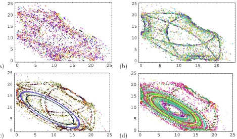
i.e., when either node 1 or 2 but neither node 3 nor 4 is dualized. A subsequent scatter plot can be made for these values, and is presented in Figure 8 for various choices of initial conditions, which are identified by different colors.

(a) 0 5 10 15 20 25 0

5 10 15 20 25

(b) 0 5 10 15 20

0 5 10 15 20 25

(c) 0 5 10 15 20 25

0 5 10 15 20 25

(d) 0 5 10 15 20 25

0 5 10 15 20 25

Figure 8: Scatter plot of (x3, x4) that are non-zero during 800 dualization steps for the initial value (32−

x3(0)−x4(0),0, x3(0), x4(0)). In each plot, (x3(0), x4(0)) is allowed to range over a rectangular region with

lower left cornerL, upper right cornerR, and minimum step size in thex3(0)and x4(0)directions equal to δ3

andδ₄ respectively. (a)L= (9,157₈),R= (10,162₈),~δ = (1₄,1₈); (b) L= (9,153₈), R= (10,156₈),~δ= (1₄,1₈); (c) L= (2,6), R= (5,9),~δ = (1,1); (d)L= (7,11),R = (9,17), ~δ(1,1₂). We use a different color for every set of initial conditions.

of [5], the entire RG flow takes place within a single toric island. The next section will be devoted to a detailed study of this case. Other trajectories jump among three squashed ellipses. These cascades consist of both quivers with r = (1,1,1,1) andr = (2,1,1,1) (and its permutations) and correspond to hopping around the six toric islands. Finally, other flows have a diffuse scatter plot, and correspond to cascades that travel to quivers with arbitrarily large gauge groups. Outside the stable elliptical orbits, numerically we find sensitive dependence on the initial conditions.

be a glued set of tetrahedra. The ellipses we observe are sections thereof. In the above plots, we have actually superimposed different surfaces, x2 = 0 and x1 = 0, but a symmetry has kept the

picture from getting muddled.

4.2.2 Analytical Evolution

Let us follow the RG flow analytically through several Seiberg dualities. We will focus on a particular sequence of dualities which repeats the sequence of dualizations on nodes 3, 1, 4 and 2. We will check later that this is indeed a consistent cascade that takes place once the initial conditions are chosen appropriately. This set of dualizations never changes the quiver, but merely amounts to a permutation of the nodes after each step. Furthermore, after four steps the cascade returns to the original quiver, with the same ordering of the nodes, but with the ranks changed as: Ni →Ni+ 4M. Now we are ready to try to understand the regime of initial conditions which will allow for such a flow. Let the initial inverse gauge couplings be x = (x1, x2, x3, x4) and set M = 1. The change

in couplings from four steps of Seiberg dualities (3142) can be cast as a linear operation sending

x→ Mx where Mis a 4×4 matrix:

M=

     

−55/729 5/9 6440/6561 56/81

0 0 0 0

154/729 ₋5/9 ₋1265/6561 70/81 70/81 1 154/729 ₋5/9

    

 . (4.5)

In particular, _Mhas eigenvectors

λ = 0,1,−5983±1904i

√ 2

6561 . (4.6)

The zero eigenvalue has eigenvector v0 = (−5,9,−9,5), which can be used to set x2 = 0. The

eigenvalue λ = 1 has eigenvector v1 = (14,0,9,9), and corresponds to a fixed point of the flow. If x = v1, then the couplings will remain unchanged after a sequence of four Seiberg dualities. The

normalization of this vector is the same one that was used in Figure 8, where we can verify that the center of the ellipses is accordingly located at (x3, x4) = (9,9). Finally, the two complex eigenvalues,

which we note to have unit modulus, and henceforth define to be

λ± :=e

±iθ _{, (4.7)}

correspond to eigenvectors

v±:=

2 3e

±_iα

,0, e±iβ,1

where

eiα =₋1

3 + 2i√2

3 ; e

iβ ₌

−7₉ −4i √

2

9 . (4.9)

Let us take our initial couplings to be x = av1 +cv+ +c∗v− for coefficients a and c. After a

large number of Seiberg dualities, the couplings become, by (4.5),

x(n) =_Mnx=av1+cλ+nv++c∗λn−v− . (4.10)

The components ofx(n) are straightforwardly obtained, using the above expressions for the various eigenvalues, as

x1 = 14a+

4

3|c|cos(nθ+α+δ)

x2 = 0

x3 = 9a+ 2|c|cos(nθ+β+δ)

x4 = 9a+ 2|c|cos(nθ+δ) (4.11)

where we have set c=|c|exp(iδ). We see that indeed, (x3, x4) give rise to the parametric equation

for an ellipse with respect to the parameter n, in accord with the scatter plots (c) and (d) in Figure 8. However, we must ask when is the above analysis applicable, i.e., when is our dualization sequence actually the sequence followed by the RG flow. Certainly a necessary condition is that the couplingsx1, x3, andx4 remain greater than zero during the flow. Thus, we see that|c|<9a/2

with a > 0. Indeed, under the condition |c| <9a/2, an elliptical disk in the coupling plane x2 = 0

is traced. The boundary of the disk is an ellipse tangent to the x3 = 0 and x4 = 0 axes at the

points x/a = (16,0,0,16) and x/a = (16,0,16,0). This condition also appears to be sufficient, as the numerics bear out. Initial conditions violating this condition will not generate ellipses, as demonstrated by plots (a) and (b).

that a can be loosely defined at any point in the RG cascade and moreover thata should be non-increasing as we move into the IR. Recall thata∼PψR(ψ)3where the sum runs over the R-charges of all the fermions in the theory [22]. From the structure of these quiver theories, one sees that

a_∼N2 _{and moreover after a sequence of four dualities for thedP}

1 flow above, N →N−4M. Thus a is indeed decreasing as we move into the IR despite the periodic behavior of the gauge couplings.

Increments in Energy Scale One final question we can answer here is how does the RG scale grow along the flow. After a sequence of four Seiberg dualities, the RG scale changes by

∆t(n) = 4 27

106

81 x1(n) +x2(n) + 1108

729 x3(n) + 4 9x4(n)

. (4.12)

In deriving this formula, we have had to look at the effect on the couplings of each of the four Seiberg dualities individually. The process is very similar to the calculations discussed in _§ 3.2.2 and we will not repeat the details here. Using the results (4.11), one finds that

∆t(n) = 16 3 a+

25_·7

36 |c|cos(nθ+δ+γ) (4.13)

where

eiγ =−241

243 −

22i√2

243 . (4.14)

Note that ∆t >0, but that t will have oscillations on top from the cosine:

t(n) = 16

3 an+ 25_·7

36 |c|

cos(δ+γ +nθ/2) sin((n+ 1)θ/2)

sin(θ/2) . (4.15)

The previous approach can be applied to periodic KS type cascades associated to other geome-tries. In the general case, as in the F0 example of Figure 2, more than one quiver can be involved

5. Supergravity Solutions for del Pezzo Flows

In the above, we have discussed in detail the RG flows for some del Pezzo gauge theories from a purely field-theoretic point of view. This is only half of the story according to the AdS/CFT Correspondence. It is important to find type IIB supergravity solutions that are dual to these field theory flows. As already emphasized [3], the main reason to trust that Seiberg duality cascades occur for the KS solution is not the field theory analysis but that it is reproduced by a well behaved supergravity solution. The purpose of this section is to investigate these dual solutions.

Surprisingly, even without a metric for the del Pezzos, we can demonstrate the existence of and almost completely characterize some of their supergravity solutions. The solutions we find are analogous to the Klebanov-Tseytlin (KT) solution [15] for the conifold. Recall that the KS solution is well behaved everywhere and asymptotes to the KT solution in the ultraviolet (large radius). The KT solution, on the other hand, is built not from the warped deformed conifold but from the conifold itself and thus has a singularity in the infrared (small radius).

5.1 Self-Dual (2,1) Solutions

To put these type IIB SuGRA solutions in historical context, note that they are closely related to a solution found by Becker and Becker [23] for M-theory compactified on a Calabi-Yau four-fold with four-form flux. One takes the four-fold to be a three-fold X times T2 _{and then T-dualizes}

on the torus, as was done in [24, 25]. The crucial point here is that the resulting complexified three-form flux has to be imaginary self-dual and a harmonic representative of H2,1_{(X) to preserve}

supersymmetry. Gra˜na and Polchinski [14] and also Gubser [26] later noticed that the KT and KS supergravity solutions were examples of these self-dual (2,1) type IIB solutions. (Indeed, the authors of [3] also mention that their complexified three-form is of type (2,1).)

Let us briefly review the work of Gra˜na and Polchinski. The construction begins with a warped product of R3,1 _{and a Calabi-Yau three-fold X:}

ds2 =Z−1/2_η

µνdxµdxν+Z1/2ds2_X , (5.1)

where the warp factor Z = Z(p), p ∈ X, depends on only the Calabi-Yau coordinates. We are interested in the case where X is the total space of the complex line bundle O(−K) over the del Pezzo dPn. Here K is the canonical class. The manifoldX is noncompact.

There exists a class of supersymmetric solutions with nontrivial flux

G3 =F3 −

i

gs

whereF3 =dC2 is the RR three-form field strength andH3 =dB2 the NSNS three-form. To find a

supergravity solution, the complex field strength G3 must satisfy several conditions: G3 must

1. be supported only in X;

2. be imaginary self-dual with respect to the Hodge star on X, i.e., ⋆XG3 =iG3;

3. have signature (2,1) with respect to the complex structure on X; and finally,

4. be harmonic.

If these conditions are met, a supergravity solution exists such that the RR field strength F5 obeys

dF5 =−F3 ∧H3 , (5.3)

and the warp factor satisfies

(_∇2_XZ)vol(X) =gsF3∧H3 , (5.4)

where vol(X) is the volume form on X. In particular, vol(X) = r5_{dr∧ vol(Y) where Y is the}

(5 real-dimensional) level surface of the cone X. The axion vanishes and the dilaton is constant:

eφ_=g

s.

5.2 (2,1) Solutions for the del Pezzo

Let us construct such aG3 for the del Pezzos. As a first step, we construct the metric onX. Letha¯b be a K¨ahler-Einstein metric on dPn such that Ra¯b = 6ha¯b. Indeed, we only know of the existence of and not the explicit form1 _{of h}

a¯b. We want to consider the case where X is a cone over dPn. In this case, the metric on X can be written [28, 29] as

ds2_X=dr2+r2η2+r2h_a¯_bdzadz¯¯b , (5.5)

where η = 1₃dψ+σ. The one-form σ must satisfy dσ = 2ω where ω is the K¨ahler form on dPn and 0≤ψ <2π is the coordinate on the circle bundle over dPn.

Next, we describe a basis of self-dual and anti-self-dual harmonic forms ondPn.2 We begin with the K¨ahler form ω. Locally, dPn looks like C2 and 2ω ∼ dz1 ∧dz¯¯1+dz2 ∧dz¯¯2. Thus locally, it is

1_{Such a metric is known not to exist fordP}

1and dP2. See for example [27].

easy to see that ω is self-dual under the operation of the Hodge star. Because the Hodge star is a local operator, ω must be self-dual everywhere. Now, recall our dPn are Einstein. Thus

ω= 6iRa¯bdza∧dz¯

¯

b _{= 6i∂∂¯ln}√_{deth . (5.6)}

Clearly dω= (∂+ ¯∂)ω = 0 whence ω must be closed. It follows that ω is a self-dual harmonic form ondPn.

There exists a cup product (bilinear form) Q onH1,1_(dP

n) defined as

Q(φ, ξ) =

Z

dPn

φ_∧ξ , φ, ξ _∈H1,1(dPn). (5.7)

The Hodge Index Theorem states that Q has signature (+,−, . . . ,−). For dPn, h2,0 = 0 while

h1,1 _{=n+ 1, there beingn other harmonic (1,1) forms on dP}

n in addition to ω. We denote these harmonic forms as φI,I = 1, . . . , n. Let us pick a basis forQ such that

φI ∧ω = 0. (5.8)

From the above discussion of ω one sees that

0< Z

ω∧⋆ω =

Z

ω∧ω (5.9)

where the inequality follows from the definition of the Hodge star and the equality from the fact that ω is self-dual. Hence the φI span a vector space V where Qhas purely negative signature.

Recall that the Hodge star in two complex dimensions squares to one: ⋆ ⋆ φ=φ. Thus we can diagonalize ⋆onV such that ⋆φI =±φI. However, if ⋆φI =φI, then one would find

R

φI∧φI >0,

in contradiction to the fact that Q has purely negative signature on V. We conclude that the φI must all be purely anti-self-dual, ⋆φI =−φI.

With these preliminaries, it is now straightforward to construct G3. We let

F3 =

k

X

I=1

aIη∧φI , H3 =

k

X

I=1

aIgs

dr

r ∧φI , (5.10)

for expansion coefficients aI_{. Hence,}

G3 =

k

X

I=1

aI(η₋idr

r )∧φI . (5.11)

This is a solution because by construction, G3 is harmonic and is supported onX so conditions (1)

and (4) are met. Moreover, (dr/r+iη) is a holomorphic one-form on X. Therefore, G3 must have

signature (2,1) becauseφ is a (1,1) form. Furthermore, it is easy to check that ⋆XG3 =iG3. Thus,

D5-Branes The number of D5-branes in this SUGRA solution is given by the Dirac quantization condition on the RR flux. More precisely, we have an integrality condition on the integral of F3

over compact three-cycles in the level surface Y of the cone X. Given a basisHJ _{(J = 1, . . . n) of} such cycles, we impose that writing

Z

HJ

F3 = 4π2α

′

MJ _{, (5.12)}

must give integer MJ_{. From the construction of Y, it follows that H}J _{will be some circle bundle} over a curveDJ _⊂dP

n while the circumference of the circle is 2π/3. Subsequently, equation (5.12) reduces to

X

I

aI

Z

DJ

φI = 6πα

′

MJ . (5.13)

To understand the curve DJ_{, we take a closer look at the divisors that correspond to elements of}

H1,1_(dP

n). BecausedPn isP2 blown up at n points, there will be a divisor H corresponding to the hyperplane in P2 _{and exceptional divisors E}

i (i = 1, . . . , n) for each of the blow ups. Essentially

because two lines intersect at a point, Q(H, H) = H ·H = 1. From the blow-up construction, we also know that Q(Ei, Ej) =Ei·Ej =−δij. Finally, Ei·H = 0 because the blow-ups are at general position. We see explicitly that Q has signature (+,₋,₋, . . . ,₋). From Poincar´e duality, there is a one-to-one map from the differential forms ω and φI to the divisors H and Ei, which we now explore.

The first chern class ofP2 _isc1(P2_{) = 3H. By the adjunction formula, it follows thatc1(dPn) =}

3H−Pn

j=1

Ej. Locally, the first chern class can be expressed in terms of the Ricci tensor,

c1(dPn) =i

Ra¯b

2π dz

a

∧dz¯¯b , (5.14)

and then from the Einstein condition (5.6), we find that

ω = π

3c1(dPn) . (5.15)

Thus, by (5.8), the φI must be orthogonal to c1(dPn). This orthogonality condition has an aston-ishingly beautiful (and well known) consequence. The orthogonal complement of 3H₋P_jEj is the weight lattice of the corresponding exceptional Lie group _En. In this language the φI must lie in this weight lattice.

in trying to quantize the flux in a far simpler system, that of a collection of point electric charges in three dimensions. In drawing a sphere (or perhaps some shape with more complicated topology) around each charge, we want to make sure that the sphere wraps around the selected charge exactly once and no other charges.

For thedPn, this condition translates into the requirement that

Z

DJ

φI =

Z

dPn

φI ∧c1(DJ) =δIJ . (5.16)

Because φI∧ω = 0, only the component of c1(DJ) orthogonal to c1(dPn) need be defined. Let us choose c1(DJ)∧ω = 0. To avoid surrounding charges more than once, we need to make the DJ

“as small as possible”. Thus we choose the c1(DJ) to be the generators of the weight lattice. The

condition (5.16) then implies that the φI generate the root lattice. For example, for dP3, we could

choose φ1 =E1 −E2, φ2 =E2 −E3, and φ3 = H−E1−E2 −E3. Indeed, the bilinear form (5.7)

can be written in the basis _Z

dPn

φI∧φJ =−AIJ (5.17)

where AIJ is the Cartan matrix for the En root lattice.

Finally, using (5.10), (5.13) and (5.16), we can normalize F3 and H3, giving us

aJ = 6πα′

MJ ; (5.18)

hence the number MJ _{of D5-branes is fixed in our SUGRA solutions. From a perturbative point of} view, we can think of this SUGRA solution as arising from the back reaction of D5-branes wrapped around vanishing curves CI of X, which are the Poincar´e duals of the φI. This follows from the definition dF3 =PaId(η∧φI) = PaIδCI.

D3-branes Having discussed some detailed algebraic geometry for the dPn, we are now ready to quantize the number N of D3-branes as well. The condition reads, using (5.3),

Z

Y

F5 = (4π2α

′

)2N , (5.19)

where F5 =F+⋆10F, and

F =X

I,J

aIaJgsln(r/r0)η∧φI ∧φJ . (5.20)

Therefore one finds, using (5.17) and (5.18),

N = 3

2πgsln(r/r0) X

I,J

MIAIJMJ (5.21)

Warp Factor Now, recalling from [28] that forY =dPn,

Z

Y

vol(Y) = π

3

27(9−n) , (5.22)

we can use (5.10) and (5.4) to solve for the warp factor. The equation reads

∂2

∂r2 +

5

r ∂ ∂r

Z(r) = (6πα

′

gs)2

Vol(Y) 2π

3r X

I,J

MIAIJMJ . (5.23)

This yields

Z(r) = 2·3

4

9₋nα

′2_g2

s

ln(r/r0)

r4 +

1 4r4

X

I,J

MIAIJMJ . (5.24)

In short, we have found the analog of the Klebanov-Tseytlin solution, a solution that is perfectly well behaved at large radius but has a curvature singularity at small radiusZ(r∗) = 0. We envision

that there is some similar warped deformed del Pezzo solution which resolves the singularity, just as the warped deformed conifold of the KS solution resolved the singularity of the KT solution.

5.3 Gauge Couplings

In order to move towards a comparison between SUGRA and gauge theory, let us determine the gauge couplings on probe branes inserted into the geometry we have discussed above. To begin with, let us study D3-branes. Their gauge coupling is simply proportional to the string coupling,

gs, which as we have seen is constant in the self-dual (2,1) solutions. In gauge theory, this is expressed by the fact that the sum of gauge couplings (2.14) is independent of the scale.

We can also probe with D5-branes. Consider a D5-brane wrapped on a curve CI ⊂dPn ⊂ Y at a fixed radial positionr in X. We take CI to be the Poincar´e dual of the harmonic two-formφI. As is well-known (see, e.g., [30]), the gauge coupling on such a brane is related to the integral of the NS 2-form around CI by

xI =

8π2

g2

I

=− 1

2πα′_g

s

Z

CI

B2. (5.25)

Thus, using the expression for B2 by integrating H3 from (5.10), as well as the value of aJ from

(5.18), we find

xI =−3 lnr

X

J

Z

CI

φJMJ . (5.26)

This yields for the beta function

βI =

dxI

dlnr =−3(CI·CJ)M

where CI ·CJ =

R

φI ∧φJ is the intersection pairing of two-cycles in dPn and the sum on J is implied.

To compare this result with gauge theory, we first need to recall the fact from section 2.2 that a D5 brane wrapped around CI is associated with a certain combination of fractional branes that we have encoded in the vector sI = (siI). Thus, the beta function βI is related to the beta functions of the fractional branes via

βI =

X

i

si_Iβi, (5.28)

Inserting the expression forβi from (2.10), we obtain the gauge theory expression

βI = 3

X

i

si_Isi_JMJ +3

2

X

ij

si_IReijsjJMJ (5.29)

where Re is given in (2.11). Let us now use the vanishing of the beta function for the conformal theory (corresponding to putting di _=ri _{in (2.8) and using (2.10)) to rewrite the first term as}

X

i

si_Isi_J =₋1

2

X

ij

si_Isi_JReij

rj

ri . (5.30)

Using the definition of Reij in (2.11), we find the gauge theory result

βI =

3 2

X

ij

e

Rij(siIs

j J −s

i IsiJ

rj

ri)M

J

= 3 2

X

ij

fij(Rij −1)(siIsjJ +s

j

IsiJ −siIsiJ

rj

ri −s

j Is

j J

ri

rj)M

J_{. (5.31)}

To finish up and relate this long-winded expression to the intersection pairing in (5.27), we need to rely on certain results concerning baryonic U(1) charges in quiver gauge theories related to del Pezzos [2, 7, 12, 31]. First of all, these baryonic U(1) charges are in one-to-one correspondence with possible non-conformal deformations. In formulas, one can write all baryonic U(1) charges QI as a sum

QI =

X

i

qi_IQi (5.32)

whereQi is a charge associated with the nodes of the quiver and is equal to +1 for incoming arrows and ₋1 for outgoing arrows. In other words,