On the Optimal Shape Parameter for Gaussian
Radial Basis Function Finite Difference
Approximation of the Poisson Equation
Oleg Davydov
∗and Dang Thi Oanh
†‡July 26, 2011
Abstract
We investigate the influence of the shape parameter in the meshless Gaussian RBF finite difference method with irregular centres on the quality of the approx-imation of the Dirichlet problem for the Poisson equation with smooth solution. Numerical experiments show that the optimal shape parameter strongly depends on the problem, but insignificantly on the density of the centres. Therefore, we suggest a multilevel algorithm that effectively finds near-optimal shape parameter, which helps to significantly reduce the error. Comparison to the finite element method and to the generalised finite differences obtained in the flat limits of the Gaussian RBF is provided.
1
Introduction
The quality of the approximation by Gaussian and other infinitely smooth radial basis functions (RBFs) is known to strongly depend on the choice of the shape (or scaling) parameter, see for example [4, Chapter 17] and references therein. In particular, this applies to the RBF-based meshless numerical methods for solving partial differential equations.
In this paper, we investigate the choice of the shape parameter for a generalised finite difference method (RBF-FD) that employs numerical differentiation stencils gen-erated by Gaussian RBF interpolation on irregular centres. The RBF-FD methods are attracting growing attention in the literature, see for example [1, 3, 7, 11, 13, 14, 16]. Even though a theoretical justification for these methods has yet to be developed, the numerical results in the above papers show their exceptional promise. In contrast to the
∗Department of Mathematics, University of Strathclyde, 26 Richmond Street, Glasgow G1 1XH,
Scotland,[email protected]
†Department of Computer Science, Faculty of Information Technology - Thai Nguyen University,
Quyet Thang Commune, Thai Nguyen City, Viet Nam,[email protected]
‡The second author was supported in part by the National Foundation for Science and Technology
more popular weak form based methods, generalised finite differences do not require nu-merical integration that may be computationally demanding for non-polynomial shape functions on non-standard domains. Moreover, one of their main advantages is high flexibility in the choice of stencil supports, which facilitates the development of adaptive methods [3] and potentially allows to handle problems with singularities in complicated 3D domains without meshing.
We consider the Dirichlet problem for the Poisson equation in 2D with a smooth solution. RBF-FD discretisation is obtained using the centres of several uniformly re-fined triangulations to allow direct comparison with the finite element method. The stencil supports are obtained by a meshless algorithm suggested in [3], leading to the system matrices with the density of non-zero entries close to the density of the stiff-ness matrices arising from the finite element method based on linear shape functions on the same triangulations. The RBF stencil weights are obtained by solving local inter-polation problems. Because the standard interinter-polation matrices of the Gaussian RBF
ϕ(r) = e−ε2 r2
are severely ill-conditioned for small values of the shape parameter ε, special techniques are needed to allow the full range of ε [6, 8, 9, 16]. We rely on the RBF-QR method of [6] adapted to RBF interpolation with a constant term.
Our main goal is to investigate the dependence of the optimal shape parameter εopt
on various factors such as the right hand sidef of the Poisson equation, the domain, the density of the centres. The numerical experiments suggest that εopt strongly depends
on f, but varies only slightly when the domain or density is changed. Based on these observations, we introduce and investigate a multilevel algorithm for the estimation of
εopt, where the shape parameter on a set of centres Ξ is optimised with respect to the
error against a solution on a refined set of centres Ξref. Such an algorithm can be
practi-cally useful if several refinement levels are available such that the computational cost of the approximate solutions on the coarse levels is negligible comparing to the cost of the final computation on the finest level, where highly optimised shape parameter leads to a significantly more accurate solution. This high accuracy, in addition to the meshless nature of the method, may further justify its practical use despite the relatively high computational cost of the system matrix assembly. As a by-product of our investigation we also observe that the polynomial type generalised finite difference method obtained in the flat limit case ε = 0 is a competitive and rather cheap option, but its results are often significantly worse than those obtained with ε = εopt. Note that the Gibbs
and Runge phenomena [5, 10] may be responsible for the sub-optimal behaviour in and close to the flat limit case, although they are not expected for the low order numerical differentiation stencils considered in this paper.
2
RBF-FD discretisation of Poisson equation
2.1
Discretisation on irregular centres
LetD be a linear differential operator, and X ={xi}n
i=1 a fixed irregular set of centres
inRd. A linearnumerical differentiation formula for the operatorD,
Du(x)≈ n
X
i=1
wi(x)u(xi), (1)
is determined by theweights wi =wi(x). The vectorw= [w1, . . . , wn]T is calledstencil.
In thefinite difference method stencils are used for the discretisation of partial differ-ential equations. Consider the Dirichlet problem for the Poisson equation in a bounded domain Ω ⊂Rd: given a function f defined on Ω, and a function g defined on ∂Ω find
u such that
∆u = f on Ω, (2)
u|∂Ω = g. (3)
This problem can be discretised with the help of differentiation formulae (1) as follows. Let Ξ⊂Ω be a finite set of discretisation centres, ∂Ξ := Ξ∩∂Ω and Ξint := Ξ\∂Ξ.
Assume that for each ζ ∈Ξint a set Ξζ ⊂Ξ is chosen such that ζ ∈Ξζ and
Ξ = [ ζ∈Ξint
Ξζ. (4)
For each ζ ∈Ξint, choose a linear numerical differentiation formula for Laplace operator
∆,
∆u(ζ)≈ X ξ∈Ξζ
wζ,ξu(ξ), (5)
with stencil [wζ,ξ]ξ∈Ξζ, and replace (2)–(3) by the system of linear equations
X
ξ∈Ξζ
wζ,ξuˆ(ξ) = f(ζ), ζ ∈Ξint, (6)
ˆ
u(ξ) = g(ξ), ξ∈∂Ξ. (7)
If (6)–(7) is nonsingular, then its solution ˆu : Ξ→ R can be compared with the vector
u|Ξ = [u(ξ)]ξ∈Ξ of the discretised exact solution of (2)–(3).
A standard finite difference method is obtained from the above if we take Ω ⊂ R2 to be a square domain, Ξ a uniformly spaced grid, and (5) the classical 5-point differentiation formula for the Laplacian.
The performance of meshless methods heavily depends on how the local sets Ξζ (stencil supports) are chosen for each ζ ∈ Ξint. There are many algorithms in the
2.2
RBF-FD method
Let Ξζ = {x0, . . . , xn} ⊂ Rd, x0 = ζ, be a local set of discretisation centres, as in
Section 2.1. Given a positive definite function ϕ : R+ → R and a continuous function
u:Rd→R, the RBF interpolant with a constant term [2, 4, 15] is sought in the form
s(x) = n
X
j=0
ajϕj(x) +c, ϕj(x) = Φ(x−xj), Φ(x) :=ϕ(kxk), (8)
wherekxkis the Euclidean norm ofx, and the coefficients aj and care chosen such that
s(xi) =u(xi), i= 0, . . . , n,
n
X
j=0
aj = 0. (9)
Thus, the coefficients are uniquely determined as the solution of the linear system
n
X
j=0
ajΦ(xi−xj) +c=u(xi), i= 0, . . . , n,
n
X
j=0
aj = 0, (10)
written in matrix form as
ΦX 1 1T 0
a c
=
u|X 0
, ΦX := [Φ(xi −xj)]ni,j=0, 1:= [1 · · · 1]T.
The matrix ΦX is symmetric and positive definite for any set X.
The interpolant s provides a good approximation of u at x if the function u is sufficiently smooth and the set of points x0, . . . , xn ∈Rd is sufficiently dense in a neigh-bourhood ofx. Moreover, the derivatives ofsare good approximations of the derivatives of u if ϕ is sufficiently smooth [15].
According to (5), we need to numerically differentiate the Laplacian of u at x0. In
RBF-FD method, an approximation of ∆u(x0) is considered in the form
∆u(x0)≈∆s(x0) =
n
X
j=0
aj∆ϕj(x0) =
n
X
i=0
wiu(xi), (11)
where the constant c not present as it is annihilated by the Laplace operator. It is easy to see that the weights wi can be found by solving the RBF interpolation problem (8)–(9) with the data given by ∆ϕi(x0),i= 1, . . . , n,
ΦX 1 1T 0
w v
=
[∆ϕi(x0)]ni=0
0
. (12)
Indeed, if the weight vector w satisfies (12), then
n
X
j=0
aj∆ϕj(x0) =
a c
T
[∆ϕi(x0)]ni=0
0 = a c T ΦX 1 1T 0
w v
=
u|X 0 T w v = n X i=0
In this paper we restrict our attention to the Gaussian RBF ϕ(r) = e−(εr)2
, which is positive definite for any value of the shape parameter ε > 0. For this function, the matrix ΦX takes the form
ΦX = [e−ε2kxi−xjk2]n
i,j=0. (13)
The Laplacians of the shifts of the Gaussian function Φ(x) =e−ε2
kxk2
needed in (12) are given by
∆ϕi(x) = 2ε2e−ε2kx−xik2(2ε2kx−xik2−d). (14)
Note that both the constant term c and the side condition Pnj=0aj = 0 can be removed in (8)–(9) because ΦX is nonsingular for Gaussian. Respectively, in the linear system (12) the coefficientv and the last equation can be removed, leading to a simpler linear system ΦXw = [∆ϕi(x0)]ni=0. However, in general, stencils obtained this way do
not satisfy the highly desirable property Pnj=0wj = 0. and therefore we prefer to use RBF interpolants with a constant term.
Instead of the stencils derived by (12), discretisations of the Dirichlet problem may be obtained with the help of numerical differentiation of certain linear combinations of Laplacians, leading to multipoint RBF stencils considered in [3]. Another alternative is provided by the Hermite RBF stencils introduced in [16].
3
Stable computation for small
ε
Since the matrix (13) is extremely ill-conditioned for small ε, alternative approaches for solving (12) are needed in this case. Several methods are available, see [6] and references therein. We follow the RBF-QR method of [6], and adapt it to the case of RBF interpolation with a constant term.
3.1
Polar-Chebyshev functions and their Laplacians
Following [6], we consider the following polar-Chebyshev expansion of ϕk(x) =ϕ(kx−
xkk) = e−(ckx−xkk)2 with bothx and x
k in the unit disk in 2D,
ϕk(x) =
∞
X
j=0
⌊Xj/2⌋
m=0
dj,mcj,m(xk)Tj,mc (x) +
∞
X
j=0
⌊Xj/2⌋
m=1−p
dj,msj,m(xk)Tj,ms (x) (15)
where p = 0 if j is even and p = 1 if j is odd. Here, the polar-Chebyshev functions
Tc
j,m(x), Tj,ms (x) are defined in polar coordinatesx=rcosθ, y=rsinθ on the unit disk −1≤r ≤1, 0≤θ < π, by
Tj,mc (x) =Tj,m(r) cos((2m+p)θ),
Tj,ms (x) =Tj,m(r) sin((2m+p)θ), 2m+p6= 0, (16)
where
Tj,m(r) =e−ε 2
r2
r2mT
and Tn(r) = cos(narccosr) denotes the Chebyshev polynomial of degree n. The coeffi-cients dj,m, cj,m(xk) and sj,m(xk) are given by
dj,m=
ε2j 2j−2m−1(j+2m+p
2 )!(
j−2m−p
2 )!
= ε
2j 2j−2m−1(⌊j+1
2 ⌋+m)!(⌊
j
2⌋ −m)!
(17)
and
cj,m(xk) = µj,me−ε 2r2
krj
kcos((2m+p)θk)1F2(α, β1, β2, ε
4r2
k),
sj,m(xk) = µj,me−ε 2r2
krj
ksin((2m+p)θk)1F2(α, β1, β2, ε
4r2
k),
α= j−2m2+p+1, β1 =j −2m+ 1, β2 = j+2m2+p+2,
wherexk =rkcosθk,yk =rksinθk,
µj,m =
1/2 if j =m = 0,
1 if j ≥ 2 even andm = 0 orm =j/2,
2 otherwise,
and 1F2 is the hypergeometric function given by the series
1F2(α, β1, β2, ε4rk2) =
∞
X
ℓ=0
ε4ℓr2kℓ
ℓ−1
Y
q=0
α+q
(β1+q)(β2+q)
.
The series (15) is convergent for any fixed ε ≥ 0 because cj,m(xk) and sj,m(xk) are O(1) as soon as xk lies in the unit disk, and the scaling coefficients dj,m decay superexponentially as j → ∞. A justification of the above formulas as well as further details on their practical implementation can be found in [6].
For the computation of numerical differentiation stencils, we will also need to evaluate the Laplacians of the functions (16). If r 6= 0, then we can use the formula ∆u =
urr+1rur+ r12uθθ to compute these Laplacians in polar coordinates as
∆Tj,mc (x) =Vj,m(r) cos((2m+p)θ),
∆Ts
j,m(x) =Vj,m(r) sin((2m+p)θ), 2m+p6= 0,
(18)
where
Vj,m(r) = Tj,m′′ (r) + 1
rT
′
j,m(r)−
(2m+p)2
r2 Tj,m(r).
Assuming that 0 < |r| < 1, we can rewrite this expression in terms of the Chebyshev polynomialTj−2m(r) = cos((j−2m) arccosr) and its derivativeTj′−2m(r) =
j−2m
√
1−r2 sin((j− 2m) arccosr),
Vj,m(r) = e−ε2r2r2m−2n4(m−ε2r2)2−4ε2r2−(j −2m)
2r2
1−r2 −(2m+p) 2T
j−2m(r)
+4(m−ε2r2) + 1 1−r2
If m ≥ 1, then (19) can also be used when r = 0, and it follows that Vj,m(0) = 0 in this case. Indeed, Vj,m has a positive power of r as a factor if m ≥ 2, and Vj,1 =
−5pTj−2(0) = 0 since Tj−2(0) = 0 when j is odd andp= 0 when j is even.
For m= 0 we obtain from (19) for 0<|r|<1,
Vj,0(r) =e−ε
2 r2n
4ε4r2−4ε2− j
2
1−r2 −
p r2
Tj(r) +
4ε2r+ r 1−r2 +
1
r
Tj′(r)
o
,
which includes a potentially singular atr = 0 term 1rT′
j(r)− p
r2Tj(r). However,
T′
j(r)
r −
pTj(r)
r2 =
(
T′
j(r)/r if j is even, (Tj(r)/r)′, if j is odd,
which is the zero function if j = 0 or 1, and a polynomial of degree j −2 for j ≥ 2. This polynomial is odd if j is odd, and hence vanishes at r = 0. For an even j = 2k it is not difficult to calculate that limr→0Tj′(r)/r = (−1)k+1j2. Since T2k(0) = (−1)k, we
conclude thatVj,m(0) = 2(−1)k+1(2ε2+j2) ifm= 0 andj = 2k is even, andVj,m(0) = 0
in all other cases. Therefore
∆Tj,mc (0) =
(
2(−1)k+1(2ε2+j2), if m = 0 andj = 2k even,
0, otherwise. (20)
∆Tj,ms (0) = 0 in all cases. (21)
3.2
Gauss-QR basis functions
Given a set of points {x0, . . . , xn} in the unit disk, the interpolant (8) is a linear
com-bination of the functions {ϕ0, . . . , ϕn}. Due to its ill-conditioning, the basis {ϕk}nk=0 is
not suitable for the computation of the interpolant s if ε is small. Therefore, this basis has to be preconditioned. In the QR method of [6] a new basis {ψk}n
k=0 is obtained as
follows. In view of (15),
ϕ0(x)
.. .
ϕn(x)
=C·D·
Tc
0,0(x)
Tc
1,0(x)
Ts
1,0(x)
Tc
2,0(x)
Tc
2,1(x)
Ts
2,1(x)
...
=CD T(x),
where D is an infinite diagonal matrix containing the scaling coefficients dj,m, and C
is a semi-infinite matrix consisting of the coefficients cj,m(xk) and sj,m(xk) in the k-th row. Let C1 be the (n+ 1)×(n+ 1) matrix consisting of the first n+ 1 columns of C,
and let C1 =QR1 be its QR factorisation, where Q is an orthogonal and R1 an upper
triangular (n+ 1)×(n + 1) matrix. Furthermore, let D1 be the main minor of D of
order n. Assuming thatC1 (or, equivalently, R1) is non-singular, we set
ψ0 ... ψn
=D1−1R−11QT
ϕ0 ... ϕn
The basis {ψk}n
k=0 performs remarkably well in numerical tests provided in [6] and
in this paper. However, its numerical implementation does not use (22) directly, which would be numerically unstable for small ε. Instead, it is based on a truncation of the expansion (15) and subsequent cancellation of the powers ofε, as explained below. The truncation pointjmax is determined such that
max i>M Dii min
1≤i≤n+1Dii
is less than unit round-off,
whereM = 12(jmax+ 1)(jmax+ 2) is the number of terms in (15) with 0≤j ≤jmax. As
a result of the truncation, the functionsϕ0, . . . , ϕnare replaced by numerically identical functions ˜ϕ0, . . . ,ϕ˜n given by
˜
ϕ0(x)
.. . ˜
ϕn(x)
= ˜CD˜T˜(x),
where ˜C consists of the first M columns of C, ˜D is the main minor of D of order M, and ˜T(x) consists of the first M components of T(x).
Let
˜
D=
D1 0
0 D2
, C˜ = C1 C2
=Q· R1 R2
, R2 :=QTC2,
so that
˜
CD˜ =Q· R1D1 R2D2
.
The functions ψ0, . . . , ψn are numerically implemented as ˜ψ0, . . . ,ψ˜n given by
˜
ψ0(x)
... ˜
ψn(x)
=D−11R1−1QT
˜
ϕ0(x)
... ˜
ϕn(x)
= I R˜ ·T˜(x), (23)
where ˜R is defined by
˜
R:=D1−1R−11R2D2.
Moreover, ˜R is computed in a numerically stable way as explained below. Note that each ˜ψk is the sum of a polar-Chebyshev function Tj,mc (x) or Tj,ms (x) from the first n components of ˜T(x) plus a linear combination of components n+ 2 to M.
To ensure numerical stability, the matrix ˜R is computed as follows. First compute
A=R−11R2. Then the productD1−1AD2 is obtained by simultaneous scaling of the rows
of A by the diagonal entries of D−11 and scaling of its columns by the diagonal entries of D2. Therefore, a typical entryrµν of ˜R has the form rµν =d−j1,m11 dj2,m2aµν, where aµν is the corresponding entry of A, and dj1,m1, dj2,m2 are diagonal elements of D1 and D2,
respectively. This implies that j1 ≤j2, and hence by (17), rµν is given by
rµν =
ε2(j2−j1)(⌊j2+1
2 ⌋+m2)!(⌊
j2
2⌋ −m2)!
2j2−j1−2(m2−m1)(⌊j1+1
2 ⌋+m1)!(⌊
j1
2⌋ −m1)!
aµν,
which does not include negative powers of ε, thus allowing stable computation for any
3.3
Computation of Gaussian RBF-FD stencils by QR method
Ifεis small, then the matrix of the linear system (12) is ill-conditioned. We now explain how Gauss-QR basis functions can be used to precondition this system. Since
ΦX =
ϕ0(x0) · · · ϕ0(xn)
... ...
ϕn(x0) · · · ϕn(xn)
, we have ΨX :=
ψ0(x0) · · · ψ0(xn)
..
. ...
ψn(x0) · · · ψn(xn)
=D1−1R−11QTΦX.
By left-multiplying both sides of (12) by
D−11R−11QT 0
0 1
,
where0denotes the zero matrices, we obtain the following preconditioned linear system
ΨX h
1T 0
w v
=
[∆ψi(x0)]ni=0
0
, h:=D1−1R−11QT1,
which is replaced in the numerical implementation by
e
ΨX h
1T 0
w v
=
[∆ ˜ψi(x0)]ni=0
0 , (24) with e ΨX := ˜
ψ0(x0) · · · ψ˜0(xn)
... ...
˜
ψn(x0) · · · ψ˜n(xn)
.
The entries of ΨXe are computed with the help of the polar-Chebyshev functions as in (23). However, for small ε, the vector h cannot be computed directly because D1−1
involves negative powers of ε, which excessively magnifies the rounding errors. The following regularisation approach performs well in our experiments. We first replace h
by ˜h := ˜DR−11QT, where ˜D is obtained from D−1
1 by replacing by zero all entries that
exceed the reciprocal of the unit round-off. By solving forw0 in the last row of (24) and
substituting w0 elsewhere, we obtain the following linear system,
n
X
j=1
( ˜ψi(xj)−ψ˜i(x0))wj+ ˜hiv = ∆ ˜ψi(x0), i= 0, . . . , n. (25)
After normalising the last column of the matrix of this system with respect to the maximum norm, and then normalising the first row, we solve it for w1, . . . , wn and ˜
v :=v/kh˜k∞, and finally compute w0 as
w0 =−
n
X
j=1
The condition number of the normalised matrix of (25) was comparable to the condi-tion number of ΨXe in all numerical tests, which shows that this method successfully eliminates the problem arising from the bad scaling ofh. It is easy to see that the above method is also applicable when ε = 0.
In view of (23), the values ˜ψi(xj) are obtained by evaluating the polar-Chebyshev functionsTc
j,m, Tj,ms , and ∆ ˜ψi(x0) require ∆Tj,mc (x0) and ∆Tj,ms (x0) according to
[∆ ˜ψi(x0)]ni=0 =
I R˜ ·∆ ˜T(x0).
To use the polar-Chebyshev expansion (15) we need to ensure that the centresx0, . . . , xn are in the unit disk. Moreover, the Laplacians of Tc
j,m, Tj,ms are faster to evaluate at the origin by using (20)–(21) than at any other points by (18)–(19). Therefore, in general, if the centres are not located in the unit disk, a linear transform of the independent variables, for example
y = (x−x0)/µ, µ:= 2 max
1≤i≤nkxi−x0k,
is needed before applying the QR method. The new centres
yj = (xj −x0)/µ, j = 0, . . . , n,
are in the unit disk, and y0 = 0. It is easy to see that the Gaussian numerical
differ-entiation stencil w of (12), with the shape parameter ε, satisfies w= ˜w/µ2, where ˜w is
obtained by solving
ΦY 1
1T 0 ˜
w
˜
v
=
[∆ϕi(0)]ni=0
0
, (26)
with the shape parameter set to µε. Hence, w can be computed by applying the QR method to (26) and then rescaling the stencil ˜w.
Since the functions ψ0, . . . ψn can only be generated by (22) if the matrixR1 is
non-singular, we always compute the condition number of R1, and only proceed if it does
not exceed a tolerance value of 1012. However, in the numerical experiments described
below in Sections 4 and 5 this value has never been exceeded. If R1 is singular or
ill-conditioned, then the QR factorisation C1 =QR1 has to be adjusted by using selective
column pivoting as described in [6].
4
Optimal shape parameter
In this section we investigate numerically the performance of the Gaussian RBF-FD method depending on the choice of the shape parameterε.
4.1
Test Problems
We consider the Dirichlet problem (2)-(3) on four domains listed below, with the right hand sides given by the functions f1–f8 and boundary conditions defined by the
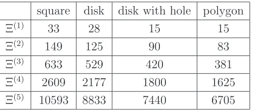
Ω we consider five sets of discretisation centres Ξ = Ξ(1), . . . ,Ξ(5) generated as
fol-lows. First, an initial triangulation T(1) is computed using MATLAB PDE Toolbox
[12] with default mesh generation parameters. This triangulation is uniformly refined four times, which produced the triangulations T(2), . . . ,T(5). The sets of discretisation
centres Ξ(1), . . . ,Ξ(5) consist of all vertices of corresponding triangulations. The number
of interior centres for each Ξ(i) is shown in Table 2.
Domains: (a) the square (−1,1)2, (b) the unit disk r < 1, (c) the unit disk with a
square hole (−0.4,0.4)2, and (d) a polygonal domain shown in Figure 3 (right). Some
of the triangulations are illustrated in Figures 1–3.
exact solution right hand side
u1(x, y) = sin(πx) sin(πy) f1(x, y) =−2π2sin(πx) sin(πy)
u2(x, y) =e−(x−0.1)
2
−0.5y2
f2(x, y) =e−(x−0.1)
2
−0.5y2
(y2+ (−2x+ 0.2)2−3)
u3(x, y) =excosy f3(x, y) = 0
u4(r, φ) =r2(r−1) sin(2φ) f4(r, φ) = 5rsin(2φ)
u5(x, y) = sin(2xy) f5(x, y) =−4 sin(2xy)(x2+y2)
u6(x, y) = sin(2π(x−y)) f6(x, y) =−8π2sin(2π(x−y))
u7(x, y) = sin(x3y) +ex−x/(1 +y2) f7(x, y) =−9 sin(x3y)x4y2+ 6 cos(x3y)xy+ex
−sin(x3y)x6− 8xy2
(1+y2)3 +(1+2yx2)2
[image:11.595.86.526.224.394.2]u8(x, y) = 12u1(x, y) +u2(x, y) f8(x, y) = 12f1(x, y) +f2(x, y)
Table 1: Test functionsu1, . . . , u8(exact solutions of the test problems) and their
Lapla-cians (right hand sides for the test problems) fi = ∆ui, i = 1, . . . ,8. The functions u4
and f4 are given in polar coordinates.
square disk disk with hole polygon
Ξ(1) 33 28 15 15
Ξ(2) 149 125 90 83
Ξ(3) 633 529 420 381
Ξ(4) 2609 2177 1800 1625
Ξ(5) 10593 8833 7440 6705
Table 2: Number of interior centres for each discretisation.
4.2
Numerical experiments
[image:11.595.182.432.483.593.2]−1 −0.5 0 0.5 1 −0.8
−0.6 −0.4 −0.2 0 0.2 0.4 0.6 0.8
−1 −0.5 0 0.5 1 −0.8
−0.6 −0.4 −0.2 0 0.2 0.4 0.6 0.8
[image:12.595.94.521.89.223.2]−1 −0.5 0 0.5 1
Figure 1: Initial triangulation T(1) and its two uniform refinements T(2),T(3) for the
square domain. The sets of discretisation centres Ξ(i) are given by the vertices of the
respective triangulations.
−1 −0.5 0 0.5 1 −0.8
−0.6 −0.4 −0.2 0 0.2 0.4 0.6 0.8
−1 −0.5 0 0.5 1 −0.8
−0.6 −0.4 −0.2 0 0.2 0.4 0.6 0.8
[image:12.595.85.528.326.460.2]−1 −0.5 0 0.5 1
Figure 2: Initial triangulation T(1) and its two uniform refinements T(2),T(3) for the
disk.
−1 −0.5 0 0.5 1
−0.8 −0.6 −0.4 −0.2 0 0.2 0.4 0.6 0.8
−1 −0.5 0 0.5 1
−0.8 −0.6 −0.4 −0.2 0 0.2 0.4 0.6 0.8
Figure 3: Initial triangulationT(1) for the disk with a square hole and for the polygonal
[image:12.595.160.466.549.671.2]the values of the exact solution on Ξint,
rmse:= 1
#Ξint
X
ξ∈Ξint
(ˆu(ξ)−u(ξ))21/2. (27)
Apart from the RBF-FD solutions, this formula applies to the standard linear finite element method with midpoint quadrature rule on the corresponding triangulationT(i).
We will use rmse of the finite element method as reference. For the RBF-FD method, we consider in addition the rms error of the numerical differentiation formula (5), given by
rmsed := 1
#Ξint
X
ζ∈Ξint
r2ζ1/2, rζ = ∆u(ζ)−
X
ξ∈Ξζ
wζ,ξu(ξ). (28)
For eachζ ∈Ξint, we select the stencil supports Ξζby a meshless algorithm described
in [3, Algorithm 1] with the target size of Ξζ\ {ζ} set to 6. This leads to Ξζ consisting of either 7 or 6 points, depending on the local geometric constellation of Ξ around ζ. Since the triangulations T(i) are quasi-uniform, Ξ
ζ obtained by this method are only rarely different from the set of vertices of all triangles sharing ζ as a vertex, that is the stencil supports of the linear finite element method. We do not provide matrix density plots similar to those in [3, Figure 11b] because the curves for the finite element stencil supports on one hand and meshless stencil supports on the other hand are not distinguishable on the triangulations considered in this paper. Therefore the comparison of the errors to those obtained by the linear finite element method is fair. In fact, from our experience, using finite element stencil supports leads to results very similar to the ones described below, but we prefer to use a meshless method for choosing Ξζ.
Since the direct method of calculation of Gaussian RBF-FD stencils by solving (12) fails for small ε because of ill-conditioning, and because Gauss-QR method is more expensive for large ε, we choose for each set Ξ(i) a ‘safe’ value ε
dmin that guarantees
that the condition number of the matrix of the system (12) does not exceed 1012for any
local set Ξζ if ε ≥ εdmin. The values of εdmin are given in Table 3. In the experiments
in this paper we always use the RBF-FD method directly if ε ≥εdmin, and we use QR
method ifε < εdmin. To compute the Gauss-QR stencils we have adapted the MATLAB
code provided in [6] and available for download fromhttp://user.it.uu.se/~bette/ research.html
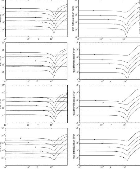
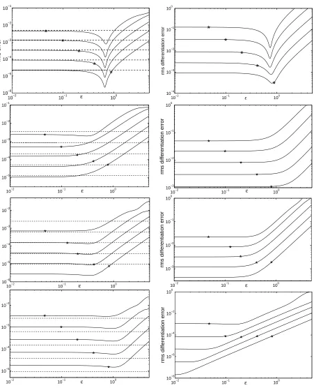
Figures 4 and 5 and Tables 4 and 5 present the results for the test function u1 on
all domains and sets of centres. In particular, Figure 5 compares the optimal rms error of Gaussian RBF-FD with the error of the finite element method, the error obtained if choosing the ‘safe’ shape parameter, and the error in the ‘flat limit’ case of ε = 0. Further results, for the test functions u2–u8, are presented in Figures 6 and 7.
We can make the following observations from these numerical experiments.
• The optimal value of the shape parameterεopt depends on the test function.
How-ever, it does not vary much when the number of centres or even the domain is changed.
• The errors with ε = εopt or even ε = 0 are always comparable with the error of
square disk disk with hole polygon Ξ(1) 0.045 0.047 0.052 0.046
Ξ(2) 0.096 0.099 0.112 0.100
Ξ(3) 0.203 0.203 0.225 0.207
Ξ(4) 0.401 0.418 0.455 0.418
[image:14.595.182.432.91.204.2]Ξ(5) 0.819 0.819 0.890 0.890
Table 3: ’Safe’ shape parameter εdmin for each discretisation.
square disk disk with hole polygon
Ξ(1) 1.36 [1.22,1.49] 1.40 [1.21,1.59] 1.33 [1.09,1.54] 1.39 [1.00,1.75]
Ξ(2) 1.32 [1.14,1.47] 1.34 [1.21,1.45] 1.31 [1.15,1.45] 1.33 [0.88,1.67]
Ξ(3) 1.31 [1.15,1.46] 1.31 [1.20,1.41] 1.31 [1.17,1.44] 1.31 [0.87,1.63]
Ξ(4) 1.31 [1.16,1.45] 1.30 [1.20,1.39] 1.30 [1.17,1.42] 1.31 [0.92,1.61]
Ξ(5) 1.32 [1.16,1.46] 1.29 [1.19,1.39] 1.30 [1.17,1.43] 1.30 [0.85, 1.63]
Table 4: Optimal shape parameters for the rms error of the solution ˆu for the test function u1. For each domain, the number in the first column is the optimal shape
parameter, whereas the second column indicates the range of values of the shape pa-rameter, for which the rms error is at most twice the optimal error.
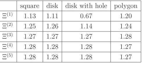
square disk disk with hole polygon
Ξ(1) 1.13 1.11 0.67 1.20
Ξ(2) 1.25 1.26 1.14 1.24
Ξ(3) 1.27 1.27 1.27 1.28
Ξ(4) 1.28 1.28 1.28 1.27
[image:14.595.185.431.547.656.2]Ξ(5) 1.28 1.28 1.28 1.27
Table 5: Optimal shape parameters for the rms differentiation error for the test function
10−2 10−1 100 10−4
10−3 10−2 10−1 100
ε
rms error
10−2 10−1 100
10−4 10−3 10−2 10−1 100 101
ε
rms differentiation error
10−2 10−1 100
10−4 10−3 10−2 10−1 100
rms error
ε 1010−2 10−1 100
−4
10−3 10−2 10−1 100 101
ε
rms differentiation error
10−2 10−1 100
10−4 10−3 10−2 10−1 100
ε
rms error
10−2 10−1 100
10−4 10−3 10−2 10−1 100 101
ε
rms differentiation error
10−2 10−1 100
10−4 10−3 10−2 10−1 100
ε
rms error
10−2 10−1 100
10−4 10−3 10−2 10−1 100 101
rms differentiation error
[image:15.595.84.535.75.620.2]ε
Figure 4: Left: The rms error of the Gaussian RBF-FD solutions for the test function
u1 on five sets of centres as a function of the shape parameterε(solid lines) compared to
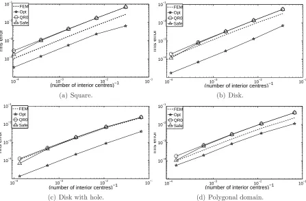
10−4 10−3 10−2 10−1 10−4
10−3 10−2 10−1
(number of interior centres)−1
rms error
FEM Opt QR0 Safe
(a) Square.
10−4 10−3 10−2 10−1
10−4 10−3 10−2 10−1
(number of interior centres)−1
rms error
FEM Opt QR0 Safe
(b) Disk.
10−4 10−3 10−2 10−1
10−4 10−3 10−2 10−1
(number of interior centres)−1
rms error
FEM Opt QR0 Safe
(c) Disk with hole.
10−4 10−3 10−2 10−1
10−4 10−3 10−2 10−1
(number of interior centres)−1
rms error
FEM Opt QR0 Safe
[image:16.595.83.530.216.510.2](d) Polygonal domain.
Figure 5: The rms error of the Gaussian RBF-FD solutions for the test function u1 on
five sets of centres as function of the number of degrees of freedom, for three values of the shape parameter: Safe refers toε=εdmin, as shown in Table 3, QR0refers toε= 0,
10−2 10−1 100 10−6
10−5 10−4 10−3 10−2 10−1
rms error
ε 10−2 10−1 100
10−4
10−3
10−2
10−1
100
ε
rms differentiation error
10−2 10−1 100
10−5 10−4 10−3 10−2 10−1
ε
rms error
10−2 10−1 100
10−3 10−2 10−1 100
ε
rms differentiation error
10−2 10−1 100
10−6 10−5 10−4 10−3 10−2
rms error
ε 10−2 10−1 100
10−3 10−2 10−1 100
ε
rms differentiation error
10−2 10−1 100
10−5 10−4 10−3 10−2
ε
rms error
10−2 10−1 100
10−8 10−6 10−4 10−2 100
ε
[image:17.595.87.538.92.648.2]rms differentiation error
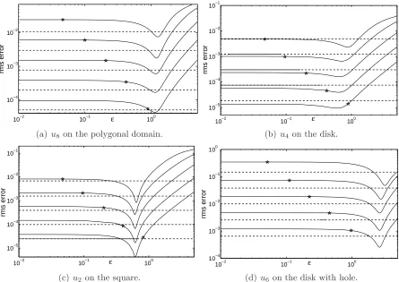
Figure 6: The rms error of the Gaussian RBF-FD solutions (left) and the rms differen-tiation error (right) as in Figure 4. From top to bottom: u2 on the polygonal domain,
10−2 10−1 100 10−4
10−3 10−2
rms error
ε
(a) u8 on the polygonal domain.
10−2 10−1 100
10−5 10−4 10−3 10−2 10−1
ε
rms error
(b) u4on the disk.
10−2 10−1 100
10−5 10−4 10−3 10−2 10−1
ε
rms error
(c) u2 on the square.
10−2 10−1 100
10−4 10−3 10−2 10−1 100
ε
rms error
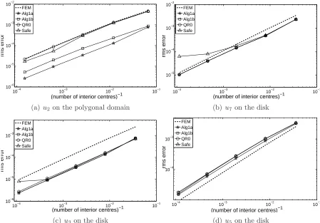
[image:18.595.83.528.220.535.2](d) u6on the disk with hole.
Figure 7: The rms error of the Gaussian RBF-FD solutions for the test functions
is refined. If the error for εopt is significantly better than the error with ε = 0,
then it is normally also significantly better than the FEM error.
• For certain test functions ε = 0 is optimal on some sets of centres, whereas a non-zero optimal value can be found on others. In these cases however, εopt does
not perform significantly better than ε = 0, so that the latter is nevertheless near-optimal.
• The ‘safe’ shape parameter gives results close toε= 0 on coarse sets of centres, but it becomes an increasingly dangerous strategy when the set of centres is refined, even though in some situations it happens by chance to be close to optimal.
• The value ofε optimal for the PDE error correlates well with the optimal value of
ε for the numerical differentiation.
• It seems difficult to predict the value of the optimal shape parameter other than by numerical experiments. It is interesting to compare εopt ≈ 1.3 for u1 and 0.7
foru2, withεopt ≈1.1 foru8 = 12u1+u2. Further experiments have shown that for
the test problems with exact solution au1+u2 with 0≤a≤1 the optimal shape
parameter lies between 0.7 and 1.3, for example εopt ≈ 0.7 if a= 0.05, εopt ≈0.9
if a= 0.2, εopt ≈1.3 ifa = 1.
5
Estimation of optimal shape parameter
Based on the observations at the end of the previous section, we suggest a multilevel algorithm for the estimation of the optimal shape parameter. It iteratively minimises a cost function defined with the help of either rms error between two solutions on a coarse and a fine set of centres, or the error of the numerical differentiation of a fine solution using the stencils generated on the coarse set of centres.
Let Ξ and Ξref be two sets of centres such that Ξ ⊂ Ξref, and ε, ε
ref two values of
the shape parameter. Denote by ˆu(respectively, ˆuref) the Gaussian RBF solution of the
Dirichlet problem (2)–(3) with the shape parameter ε on Ξ (respectively, εref on Ξref).
As explained above, the stencils to set up the system can be computed either directly or by the QR method. Clearly, ˆuref can be restricted to Ξ. Our first cost function is
given by the root mean square distance between two approximate solutions on the set of centres Ξ,
cost(ε, εref) :=
1
#Ξint
X
ξ∈Ξint
(ˆu(ξ)−uˆref(ξ))2
1/2
. (29)
The second approach is to measure the accuracy of the RBF numerical differentiation formulae on the set Ξ, obtained with the shape parameter value ε,
∆u(ζ)≈ X ξ∈Ξζ
against the ones on the refined set of centres Ξref, obtained with the shape parameter
value εref,
∆u(ζ)≈ X ξ∈Ξref
ζ
wrefζ,ξu(ξ), ζ ∈Ξrefint.
The error between two approximate Laplacians of ˆuref at ζ ∈Ξint is given by
eζ =
X
ξ∈Ξζ
wζ,ξuˆref(ξ)−
X
ξ∈Ξref
ζ
wrefζ,ξuˆref(ξ),
and this leads to the second cost function in the form
cost(ε, εref) :=
1
#Ξint
X
ζ∈Ξint
e2ζ1/2. (30)
Note that (30) is cheaper to compute than (29), especially if Ξref is fixed and Ξ varies,
since (30) does not require the knowledge of the approximate solution ˆuof the Dirichlet problem on Ξ.
Underlying assumption is that the optimal shape parameters for two sets of centres are close together as observed in the numerical results of the previous section.
Algorithm 1. Estimation of optimal shape parameter using approximate so-lution on a refined set of centres. Options (referred to as Algorithm 1a and
Algorithm 1b, respectively): (a)the cost function is defined by (29), and(b)the cost function is defined by (30). Input: two sets of centres Ξ,Ξref such that Ξ ⊂ Ξref and
initial estimate of the optimal shape parameter εref. Output: estimated optimal shape
parameter εopt. Parameters: tolerances λ > δ > 0, maximum number of iterations m,
upper bound C for the shape parameter. In the numerical tests below the following parameter values have been used: δ= 0.01,λ= 0.1, m= 4, and C = 5.
I. Compute Gaussian RBF solution ˆuref on Ξref with shape parameter εref and find
ε ∈ [εmin, εmax] such that cost(ε, εref) is minimised, where [εmin, εmax] = [0, C] if
εref = 0 and [εmin, εmax] = [εref−λ, εref+λ] otherwise.
II. For i= 1, . . . , m:
If |ε−εref|< δ: STOP and return εopt =ε.
ElseIf ε=εmin orε =εmax: STOP and returnεopt=NaN.
Else: Set εref =ε and repeat Step I.
Return: εopt= NaN
Remarks
1. Algorithm 1 fails if it returnsNaN. If this happens with inputεref >0, this indicates a
wrong initial estimate of the shape parameter and a remedy is to rerun Algorithm 1 with εref = 0. If however NaN is returned with input εref = 0, then the likely reason
is that the solution ˆuref is not sufficiently accurate, and we suggest to replace Ξref by
2. In our numerical tests with the sets Ξ(1), . . . ,Ξ(5), Algorithm 1 reliably computes
nearly optimal shape parameter if Ξref = Ξ(n+1) for Ξ = Ξ(n) when Ξ(n) is sufficiently
fine. However, for a coarse set of centres this may be unreliable and a larger gap between Ξ and Ξref is needed. Therefore, we apply Algorithm 1 as follows: First run
it with Ξ = Ξ(1), Ξref = Ξ(3), ε
ref = 0, to obtain a nearly optimal shape parameter
ε1 for Ξ(1). Then run it with εref = ε1, Ξ = Ξ(2), Ξref = Ξ(3), to obtain a nearly
optimal shape parameter ε2 for Ξ(2). If Algorithm 1 fails and returns NaN (which
happened extremely rare in our tests), then set εref = 0 and rerun Algorithm 1. In
our tests Algorithm 1 never failed with εref = 0. The value ε2 is also used on the
sets Ξ(3),Ξ(4),Ξ(5). Therefore, multiple values of ε are only tested on Ξ(1),Ξ(2),Ξ(3),
which is cheaper than the cost of the computation with a single ε on Ξ(5).
3. Optimisation with respect toε in Step I is done using MATLAB function fminbnd. We set MaxFunEvals = 9 and TolX= 10−2 to reduce computation cost.
4. Parameterm is an upper bound on the number of computations of the RBF solution on Ξref. Settingm to a small value may help to reduce the cost. However, ifm is too
small it causes unnecessary failures of the algorithm, and costly reruns with refined Ξref. In our experiments m = 4 was sufficiently large to ensure that the failures
are extremely rare. Setting C = 5 is justified by the graphs in Section 4 where the optimal shape parameter is always less than this number.
5. When computing Gaussian RBF solutions ˆu or ˆuref we either use Gauss-direct or
Gauss-QR depending on whether the shape parameter ε is smaller than the smallest safe valueεdmin for which the condition number of the matrix of (12) does not exceed
1012, see Table 3. If the interval [ε
min, εmax] includesεdmin, then we further reduce cost
by first running fminbnd in the interval [εdmin, εmax] using Gauss-direct, and then,
only if εdmin is optimal in this interval, we run fminbnd in the interval [εmin, εdmin]
using Gauss-QR.
Numerical experiments
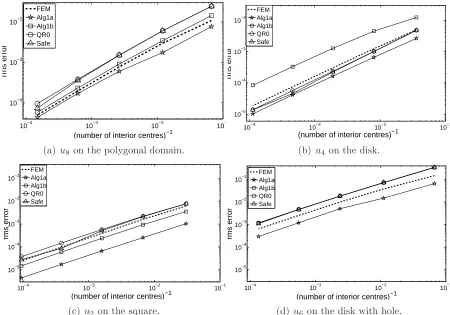
Figures 8–10 and Tables 6–8 below illustrate the performance of Algorithm 1 for the test problems in Figures 4, 6 and 7. In these experiments Algorithm 1a effectively finds near-optimal shape parameter, whereas Algorithm 1b sometimes returns sub-optimal, albeit acceptable results. The tables also confirm that the number of iterations needed in Step II is small, typically just 2 or 3.
6
Conclusion and future work
10−4 10−3 10−2 10−1 10−4
10−3 10−2 10−1
(number of interior centres)−1
rms error
FEM Alg1a Alg1b QR0 Safe
(a) u1 on the square
10−4 10−3 10−2 10−1
10−4 10−3 10−2 10−1
(number of interior centres)−1
rms error
FEM Alg1a Alg1b QR0 Safe
(b) u1on the disk
10−4 10−3 10−2 10−1
10−4 10−3 10−2 10−1
(number of interior centres)−1
rms error
FEM Alg1a Alg1b QR0 Safe
(c) u1 on the disk with hole
10−4 10−3 10−2 10−1
10−4 10−3 10−2 10−1
(number of interior centres)−1
rms error
FEM Alg1a Alg1b QR0 Safe
[image:22.595.84.529.199.508.2](d) u1on the polygonal domain
Figure 8: The rms error of the Gaussian RBF-FD solutions for the test function u1
10−4 10−3 10−2 10−1 10−6
10−5 10−4 10−3 10−2
(number of interior centres)−1
rms error
FEM Alg1a Alg1b QR0 Safe
(a) u2 on the polygonal domain
10−4 10−3 10−2 10−1
10−5 10−4 10−3 10−2
(number of interior centres)−1
rms error
FEM Alg1a Alg1b QR0 Safe
(b) u7on the disk
10−4 10−3 10−2 10−1
10−6 10−5 10−4 10−3
(number of interior centres)−1
rms error
FEM Alg1a Alg1b QR0 Safe
(c) u3on the disk
10−4 10−3 10−2 10−1
10−4 10−3
(number of interior centres)−1
rms error
FEM Alg1a Alg1b QR0 Safe
[image:23.595.81.530.213.526.2](d) u5on the disk
10−4 10−3 10−2 10−1 10−4
10−3 10−2
(number of interior centres)−1
rms error
FEM Alg1a Alg1b QR0 Safe
(a) u8 on the polygonal domain.
10−4 10−3 10−2 10−1
10−5 10−4 10−3 10−2
(number of interior centres)−1
rms error
FEM Alg1a Alg1b QR0 Safe
(b) u4on the disk.
10−4 10−3 10−2 10−1
10−5 10−4 10−3 10−2 10−1
(number of interior centres)−1
rms error
FEM Alg1a Alg1b QR0 Safe
(c) u2 on the square.
10−4 10−3 10−2 10−1
10−5 10−4 10−3 10−2 10−1
(number of interior centres)−1
rms error
FEM Alg1a Alg1b QR0 Safe
[image:24.595.80.530.215.530.2](d) u6on the disk with hole.
square disk disk with hole polygon
εopt nIter εopt nIter εopt nIter εopt nIter
Algorithm 1a 1.31 2 1.35 2 1.31 2 1.33 2
[image:25.595.112.496.70.143.2]Algorithm 1b 1.25 2 1.25 3 0.91 4 1.24 2
Table 6: The near optimal shape parameter εopt and the number of iterations nIter in
Step II of Algorithm 1 when Ξ = Ξ(2) and Ξref = Ξ(3) (see Remark 2 after Algorithm 1)
for the test function u1.
u2 polygonal u7 disk u3 disk u5 disk
εopt nIter εopt nIter εopt nIter εopt nIter
Algorithm 1a 0.69 2 0 2 0.31 3 0.93 4
[image:25.595.121.493.214.288.2]Algorithm 1b 0.74 2 0 1 0.17 2 0 1
Table 7: The near optimal shape parameterεopt and the number of iterations nIter as
in Table 6 for the test functions and domains as in Figures 6 and 9.
an algorithm to estimate the optimal shape parameter by comparing RBF-FD solutions on two sets of centres and verified it numerically on the same test problems. Our tests with the full range of the shape parameters, including the flat limit at ε = 0 were possible thanks to the recent QR method [6] which we adapted to the interpolation with a constant term and computation of Gaussian RBF-FD stencils.
Apparently, it is difficult to explain this phenomenon theoretically and develop ana-lytic methods to determine the optimal shape parameter for a given right hand side of the Poisson equation. Further work is needed to see whether this behaviour persists for other types of equations, non-Dirichlet boundary conditions or 3D problems, as well as for other radial basis functions.
The case ε= 0 seems of independent interest because, computed by QR method, it is effectively a polynomial rather than RBF method. It was sometimes optimal and in general competitive in our experiments. Its computational cost is the lowest of any ε
requiring QR method [6].
Higher order stencils
In our experiments we used stencil supports generated by [3, Algorithm 1] which contain just 6 or 7 points as they are designed to compete with the finite element method based on linear shape functions. Therefore it is important to investigate whether the optimal shape parameter is still indifferent to domain shapes and densities of centres if larger stencils are employed. Figure 11 presents results of an initial test in this direction, confirming that this is likely to be the case. Here, the Poisson equation with the right hand side and Dirichlet boundary conditions derived from the exact solution
u1 of Table 1 was solved on the square domain with centres generated by the same
u8 polygonal u4 disk u2 square u6 disk with hole
εopt nIter εopt nIter εopt nIter εopt nIter
Algorithm 1a 1.21 4 0.73 4 0.61 3 2.82 2
[image:26.595.105.509.71.142.2]Algorithm 1b 0.84 3 1.91 4 0.74 2 0.38 4
Table 8: The near optimal shape parameterεopt and the number of iterations nIter as
in Table 6 for the test functions and domains as in Figures 7 and 10.
new set of centres Ξe(i) associated with T(i) includes vertices and midpoints of edges of
the triangulation T(i), which implies Ξe(i) = Ξ(i+1) because T(i+1) is obtained by the
uniform refinement of T(i). Obviously, Ξe(i) is the set of centres corresponding to the
finite element method with quadratic shape functions on T(i), and the corresponding
stencil support selection method includes into Ξe(ζi) all points of Ξe(i) lying in the union
of the triangles of T(i) containing ζ ∈ Ξe(i). Thus, Ξe(i)
ζ consist of 9 points if ζ is the middle point of an edge of T(i) and 3n+ 1 points if ζ is an interior vertex connected
to n other vertices of T(i). We have solved the Dirichlet problem with Gaussian
RBF-FD method using finite element stencil supports eΞ(ζi). Figure 11 provides the rms error of this solution and the rms differentiation error. The stars on the first three curves indicate the position of the ‘safe’ε=εdmin, so that the QR method is used to the left of
these points. Note that the values ofεdmin are now higher than those in Table 3 because
larger stencils are used. The fourth curve (for Ξe(4)) is completely obtained by the QR
method. We observe that the optimal shape parameter for the solution and numerical differentiation errors is about 1.3 for all Ξe(i), i = 1, . . . ,4, which is close to the values
obtained for u1 in Section 4, see Figure 4 and Table 4. We can also see that the errors
are significantly better than those obtained with the same number of centres for the same problem in Section 4, as expected from larger stencils. However, Figure 11 does not seem to indicate a higher convergence order. Clearly, further research is needed on meshless stencil support selection algorithms leading to stencils of size comparable with higher order finite element methods and delivering comparably accurate RBF-FD solutions.
Adaptive centres
For practical applications it is important to determine good shape parameters for more complex right hand sides, where typically distributions of centres with spatially varying densities are needed. In [3] we tested RBF-FD methods on adaptive centres generated by adaptive refinement for the Dirichlet problem (2)–(3), where the domain Ω is the disk sector defined by the inequalities r < 1, −3π/4 < ϕ <3π/4 in polar coordinates, the right hand side f = 0, the boundary conditions are defined by g(r, ϕ) = cos(2ϕ/3) along the arc, and g(r, ϕ) = 0 along the straight lines. The exact solution is u(r, ϕ) =
r2/3cos(2ϕ/3). Figure 12 and Table 9 present the results of new experiments for several
10−2 10−1 100 10−4
10−3 10−2
ε
rms error
10−2 10−1 100
10−4 10−3 10−2 10−1 100
ε
[image:27.595.84.524.70.208.2]rms differentiation error
Figure 11: The rms error of the Gaussian RBF-FD solutions (left) and the rms numerical differentiation error (right) for the test functionu1 on the square using stencil supports
of the quadratic finite element method.
depicts the rms error of the Gaussian RBF-FD solution against the exact solution for two versions of the shape parameter: ε = 0 and optimal ε = εopt found by minimising the
rms error. Recall that in [3] the shape parameter was chosen individually for each stencil as the smallest ‘safe’ ε with the property that the condition number of (12) does not exceed 1012. Comparing Figure 12 with the curve for Gaussian RBF in [3, Figure 10a], we
observe that the results are very close. In particular, the optimal shape parameter shows no significant advantage over ε = 0 for this test function, similar to what we found for
u3, u5, u7 on uniform refinements in Section 4. Table 9 gives more detailed information
about the values of the optimal shape parameter and corresponding errors. Note that choosing a single value of the shape parameter everywhere in the domain may not be the right approach for functions with singularities or spatially varying smoothness. We hope nevertheless that the results of this paper will help develop effective shape parameter selection algorithms for more complicated problems in the future.
Acknowledgements
We are grateful to two anonymous referees for useful suggestions that have helped to improve the paper. The second author thanks Professor Hoang Xuan Phu for stimulating discussions.
References
[1] J. P. Boyd and L. Wang. Truncated Gaussian RBF differences are always inferior to finite differences of the same stencil width. Commun. Comput. Phys., 5:42–60, 2009.
[2] M. D. Buhmann. Radial Basis Functions. Cambridge University Press, New York, NY, USA, 2003.
10−2 10−4
10−3
(number of interior centres)−1
rms error
[image:28.595.150.458.89.281.2]FEM QR0 Opt
Figure 12: The rms error of the Gaussian RBF-FD solutions on adaptive centres for the test problem described in Section 6: The curve marked by QR0 is obtained with ε = 0 and Opt with the optimal shape parameter, whereas FEM indicates the rms error of the finite element method with linear shape functions.
#centres εopt rms error for εopt rms error for ε= 0 rms error of FEM
82 2.26 3.91e-03 4.96e-03 4.06e-03
84 0 1.43e-03 1.43e-03 4.01e-03
91 0 1.87e-03 1.87e-03 3.39e-03
99 1.03 1.44e-03 2.01e-03 2.87e-03
109 0.95 8.72e-04 1.48e-03 2.18e-03
114 0.74 1.39e-03 1.64e-03 1.92e-03
137 0.87 7.13e-04 1.24e-03 1.57e-03
152 0.52 8.17e-04 8.97e-04 1.39e-03
187 0.38 3.67e-04 3.95e-04 1.05e-03
215 0.58 4.87e-04 6.13e-04 8.43e-04
290 0.32 2.45e-04 2.68e-04 6.21e-04
349 0.59 2.51e-04 3.65e-04 4.83e-04
484 0 1.17e-04 1.17e-04 3.66e-04
Table 9: The sizes of the sets of centres, values of the optimal shape parameter and the rms errors for ε = εopt, ε = 0 and FEM for the experiments on adaptive centres
[image:28.595.106.507.399.651.2][4] G. F. Fasshauer. Meshfree Approximation Methods with MATLAB. World Scientific Publishing Co., Inc., River Edge, NJ, USA, 2007.
[5] B. Fornberg and N. Flyer. The Gibbs phenomenon for radial basis functions. In A. Jerri, editor, The Gibbs Phenomenon in Various Representations and Applica-tions, pages 201–222. Sampling Publishing, Potsdam, NY, 2011.
[6] B. Fornberg, E. Larsson, and N. Flyer. Stable computations with Gaussian radial basis functions. SIAM J. Sci. Comput., 33(2):869–892, 2011.
[7] B. Fornberg and E. Lehto. Stabilization of RBF-generated finite difference methods for convective PDEs. J. Comput. Phys., 230:2270–2285, 2011.
[8] B. Fornberg and C. Piret. A stable algorithm for flat radial basis functions on a sphere. SIAM J. Sci. Comput., 30:60–80, 2007.
[9] B. Fornberg and G. Wright. Stable computation of multiquadric interpolants for all values of the shape parameter. Comput. Math. Appl., 48:853–867, 2004.
[10] B. Fornberg and J. Zuev. The Runge phenomenon and spatially variable shape parameters in RBF interpolation. Comput. Math. Appl., 54:379–398, 2007.
[11] C. K. Lee, X. Liu, and S. C. Fan. Local multiquadric approximation for solving boundary value problems. Comput. Mech., 30(5-6):396–409, 2003.
[12] Partial Differential Equation ToolboxTM User’s Guide. The MathWorks, Inc, 2009.
[13] C. Shu, H. Ding, and K. S. Yeo. Local radial basis function-based differential quadrature method and its application to solve two-dimensional incompressible Navier-Stokes equations. Comput. Methods Appl. Mech. Eng., 192(7-8):941–954, 2003.
[14] A. I. Tolstykh and D. A. Shirobokov. On using radial basis functions in a ‘finite dif-ference mode’ with applications to elasticity problems. Computational Mechanics, 33(1):68–79, 2003.
[15] H. Wendland. Scattered Data Approximation. Cambridge University Press, 2005.