Non-isothermal flow of a thin film of fluid with temperature-dependent viscosity on a stationary horizontal cylinder

Non-isothermal flow of a thin film of fluid with

temperature-dependent viscosity on a stationary horizontal

cylinder

G. A. Leslie, S. K. Wilson∗ _{and B. R. Duffy}†

Department of Mathematics and Statistics,

University of Strathclyde, 26 Richmond Street,

Glasgow G1 1XH, United Kingdom

(Dated: 30th September 2010, revised 2nd March and 2nd May 2011)

Abstract

A comprehensive description is obtained of the two-dimensional steady gravity-driven flow with prescribed volume flux of a thin film of Newtonian fluid with temperature-dependent viscosity on a stationary horizontal cylinder. When the cylinder is uniformly hotter than the surrounding atmosphere (positive thermoviscosity) the effect of increasing the heat transfer to the surrounding atmosphere at the free surface is to increase the average viscosity and hence reduce the average velocity within the film, with the net effect that the film thickness (and hence the total fluid load on the cylinder) is increased to maintain the fixed volume flux of fluid. When the cylinder is uniformly colder than the surrounding atmosphere (negative thermoviscosity) the opposite occurs. Increasing the heat transfer at the free surface from weak to strong changes the film thickness everywhere (and hence the load, but not the temperature or the velocity) by a constant factor which depends only on the specific viscosity model considered. The effect of increasing the thermoviscosity is always to increase the film thickness and hence the load. In the limit of strong positive thermoviscosity the velocity is small and uniform outside a narrow boundary layer near the cylinder leading to a large film thickness, while in the limit of strong negative thermoviscosity the velocity increases from zero at the cylinder to a large value at the free surface leading to a small film thickness.

∗ _{Author to whom correspondence should be addressed. Electronic mail: s.k.wilson@strath.ac.uk,} Tele-phone: + 44 (0) 141 548 3820, Fax: + 44 (0) 141 548 3345.

I. INTRODUCTION

The non-isothermal flow of a thin film of fluid on a heated or cooled horizontal circular

cylinder is relevant to many industrial situations, including heat exchangers and various

coating processes. Pioneering work on this problem was done by Nusselt1,2_{, who studied}

the steady condensation of a quiescent surrounding vapour (steam) into a thin film of fluid

(water) on a stationary horizontal cylinder. Extensions of this basic problem have been

considered by many subsequent authors, including, for example, Sparrow and Gregg3_{, Nicol}

et al.4 _{and Shu and Wilks}5_{, who included fluid inertia and thermal advection in the film,}

Shekriladze and Gomelauri6_{, Fujii et al.}7_{, Rose}8 _{and Chen and Lin}9_{, who considered the}

influence of flow of the vapour, and Sarma et al.10 _{and Yang and Lin}11_{, who considered}

turbulent flow in the film. Condensation onto an elliptical (rather than a circular) cylinder

has been studied by Yang and Hsu12 _{for the case of laminar flow and by Lin and Yang}13 _for

the case of turbulent flow. Another notable work on the non-isothermal flow of a thin film

of fluid on a stationary horizontal cylinder is that by Reisfeld and Bankoff14_{, who undertook}

a pioneering investigation of unsteady flow on a heated or cooled cylinder due to gravity,

surface tension, thermocapillary (i.e. variation of surface tension with temperature) and van

der Waals forces. Subsequently, Conlisk and Mao15 _{investigated the unsteady flow of a}

thin film of fluid on a horizontal cylinder accounting for condensation from the surrounding

vapour for both one-component and two-component fluids.

In a number of practical situations thermoviscosity (i.e. variation of viscosity with

tem-perature) effects are significant, and as a result there have also been a number of studies

of a variety of non-isothermal flows of fluids with temperature-dependent viscosities on a

variety of substrates. In particular, Goussis and Kelly16,17 _{and Hwang and Weng}18

inves-tigated the stability of a layer of fluid with temperature-dependent viscosity flowing down

independently considered the evolution and eventual rupture of a thin film of fluid with

temperature-dependent viscosity on a heated horizontal substrate subject to surface tension

and van der Waals forces. Selak and Lebon21 _{investigated the onset of convection in a}

qui-escent layer of fluid with temperature-dependent viscosity on a heated or cooled horizontal

substrate subject to both buoyancy and thermocapillary effects. Geophysical applications

such as lava flows have motivated the study of the radial spreading of a thin film of fluid

with temperature-dependent viscosity on a horizontal substrate by Bercovici22 _{who included}

thermal advection, and by Balmforth and Craster23 _{who considered a viscoplastic fluid with}

a temperature-dependent viscosity and yield stress. Kabova and Kuznetsov24 _{calculated the}

steady flow of a thin film of fluid with temperature-dependent surface tension and

viscos-ity down an inclined substrate. Wilson and Duffy25,26 _{and Duffy and Wilson}27 _{studied the}

steady flow of a rivulet with temperature-dependent viscosity down a heated or cooled

in-clined substrate for three viscosity models (namely a linear, an exponential and an Eyring

model). Sansom et al.28 _{considered the spreading of a thin film of fluid with}

temperature-dependent viscosity on a horizontal substrate for three viscosity models (namely a linear, an

exponential and a biviscosity model) for both a heated or cooled substrate without internal

heating within the film and for a substrate at the ambient temperature with constant internal

heating within the film. Unsteady flow of a thin film of fluid with temperature-dependent

surface tension and viscosity on a uniformly rotating disk was considered independently by

Usha et al.29 _{and Wu}30_.

There is also a considerable body of literature on both two-dimensional and

three-dimensional isothermal thin-film flow on both the inside and the outside of a horizontal

cylinder which is also of relevance here. Lin et al.31_{investigated three-dimensional evolution}

and rupture of a film due to van der Waals forces. King et al.32_{studied the three-dimensional}

evolution of a film on both a horizontal and an inclined cylinder. Band et al.33 _considered

and Oron34 _{investigated the effect of axial oscillations of the cylinder on the evolution and}

rupture of an axisymmetric film. In addition, there is a considerable and rapidly growing

body of work on isothermal thin-film flow on both the inside (often called “rimming flow”)

and the outside (often called “coating flow”) of a uniformly rotating circular cylinder

build-ing on the pioneerbuild-ing work by Moffatt35_{, Pukhnachev}36 _{and Johnson}37_{. For example, Duffy}

and Wilson38 _{considered steady “curtain” flows on the outside of both a stationary and a}

uniformly rotating cylinder, while Ashmore et al.39_{, Villegas-D´ıaz et al.}40_{and Benilov et al.}41

investigated various aspects of rimming flow, and Evans et al.42_{, Kelmanson}43 _{and Hunt}44

investigated various aspects of coating flow (the latter in the case of an elliptical cylinder).

However, despite the practical importance of the problem surprisingly little work has been

done on the steady gravity-driven flow of a thin film of fluid with temperature-dependent

viscosity on a heated or cooled horizontal cylinder. Recently Duffy and Wilson45 _examined

this problem for both a stationary and a uniformly rotating cylinder in the special case

when the free surface is at the same uniform temperature as the surrounding atmosphere

(i.e. at leading order in the limit of large Biot number). In particular, they found that in

this case the film thickness (and hence the load, but not the temperature or the velocity)

can be obtained from that in the isothermal case by a simple re-scaling. However, they

did not appreciate that other re-scalings are possible in the case of a stationary cylinder

or undertake any analysis of the solution obtained. In the present work we build on the

foundations laid by Duffy and Wilson45 _{to obtain a comprehensive description of the steady}

gravity-driven flow with prescribed volume flux of a thin film of fluid with

temperature-dependent viscosity on a heated or cooled stationary horizontal cylinder. In particular, we

investigate the effect of varying the heat transfer to or from the atmosphere at the free

II. THE VISCOSITY MODEL AND THE THERMOVISCOSITY NUMBER

So far as possible we will present results for a general viscosity model µ = µ(T), where

µ(T) is a monotonically decreasing function of temperature T satisfying (without loss of

generality) µ = µ0 and dµ/dT = −λ when T = T0, where λ > 0 is a prescribed positive

constant and T0 is the uniform temperature of the cylinder at which µ takes the constant

value µ0. However, when it is necessary to specify a particular viscosity model and, in

particular, for illustrative purposes, we adopt the widely used exponential viscosity model

µ(T) =µ0exp

−λ(T −T0)

µ0

(1)

(see, for example, Goussis and Kelly16,17_{, Hwang and Weng}18_{, Selak and Lebon}21_{, Balmforth}

and Craster23_{, and Wilson and Duffy}25_).

Regardless of the specific viscosity model under consideration, an appropriate

non-dimensional measure of thermoviscosity (i.e. the variation of viscosity with temperature)

is provided by thethermoviscosity number, V, defined by

V = λ(T0−T∞)

µ0

, (2)

whereT∞ is the uniform temperature of the atmosphere. Since the thermoviscosity number

has the same sign as T0 −T∞, situations in which the cylinder is hotter (colder) than the

atmosphere correspond to positive (negative) values of V. In practice, the magnitude of V

can vary over several orders of magnitude from arbitrarily small values (when the viscosity

is effectively independent of temperature and/or when the magnitude of the heating or

cooling is small) to reasonably large values (when the viscosity is strongly dependent on

temperature and/or when the magnitude of the heating or cooling is large). For example,

using the parameter values given by Selak and Lebon21 _{in the case |T}

0−T∞|= 25 K yields

|V_| = 0.3825 for acetic acid, _|V_| = 0.5225 for silicone oil, _|V_| = 0.625 for water, and

|V_|= 2.5125 for glycerol, while Balmforth and Craster23 _{give “typical” values of}

FIG. 1: Geometry of the problem: steady two-dimensional flow of a thin film of Newtonian fluid with temperature-dependent viscosity on a stationary horizontal cylinder which may be either uniformly hotter

or colder than the surrounding atmosphere.

wax and slurry, _|V_| = 5 for basaltic lava, _|V_| = 7 for syrup, and _|V_| = 10₋18 for silicic

lava. Hence we will consider the full range of values from V = 0 to the limits V _{→ ∞} and

V _{→ −∞} in the present work.

III. PROBLEM FORMULATION

Consider two-dimensional steady gravity-driven flow of a thin film of Newtonian fluid with

uniform density ρ and temperature-dependent viscosity µ=µ(T), where T denotes the (in

general) non-uniform temperature of the fluid, on a stationary circular cylinder of radius a

with its axis horizontal, the cylinder being at a uniform temperatureT0, which may be either

hotter or colder than the uniform temperature T∞ (6=T0) of the surrounding atmosphere.

Referred to polar coordinatesr=a+Y (with origin at the cylinder’s axis) andθ(measured

the fluid to be at r = a +h, the film thickness being denoted by h. The fluid velocity

u= ueθ+ver (where eθ and er denote unit vectors in the azimuthal and radial directions,

respectively), pressure pand temperatureT are governed by the familiar mass-conservation,

Navier–Stokes and energy equations. On the cylinderr=athe velocityusatisfies the no-slip

and no-penetration conditions, and the temperature is T =T0 (a prescribed constant). On

the free surfacer=a+hthe usual normal and tangential stress balances and the kinematic

condition apply, as does Newton’s law of cooling

−kth∇T ·n =αth(T −T∞), (3)

wherekthdenotes the thermal conductivity of the fluid (assumed constant),αth(≥0) denotes

an empirical surface heat-transfer coefficient, and n denotes the unit outward normal to

the free surface. Surface tension, viscous dissipation, inertia and thermal advection are all

neglected.

Since the flow is steady, the volume flux per unit axial length Q (measured positive in

the direction of increasing θ) is a piecewise constant, and since (as we shall show) the film

thickness h always becomes unbounded at the top (θ = π/2) and the bottom (θ = ₋π/2)

of the cylinder (where the tangential component of gravity is zero), it is natural to follow

previous studies of the isothermal problem (see, for example, Duffy and Wilson38_{) and to}

interpret this as a curtain of fluid with prescribed constant volume fluxQS(>0) falling onto

the top of the cylinder and splitting into two films with constant azimuthal fluxes Q =QR

and Q = QL round the right-hand and left-hand sides of the cylinder, respectively, with a

corresponding curtain (also with fluxQS) falling off at the bottom of the cylinder. By global

conservation of mass these fluxes are related by QS = QL −QR, but the relative split of

the flux between the two sides of the cylinder is not determined by the present theory. In

particular, the flow need not necessarily have left-to-right symmetry (i.e. QR and QL need

not necessarily be equal to₋QS/2 andQS/2, respectively).

cylinder M is denoted by M =MR and M =ML on the right-hand and left-hand sides of

the cylinder, respectively, and hence the total fluid load on the cylinder is given byMR+ML.

We will consider only thin films, whose aspect ratioǫ, defined by

ǫ=

µ0QS

ρga3

1/3

≪1, (4)

is small. We non-dimensionalise and scale the system by writing

r=a(1 +ǫY∗_{), h=ǫah}∗_{, u=Uu}∗_{, v =ǫUv}∗_,

p=pa+ǫaρgp∗, T =T∞+ (T0−T∞)T∗, µ=µ0µ∗,

Q=QSQ∗ =ǫaUQ∗, QR =QSQ∗R =ǫaUQ∗R, QL =QSQ∗L =ǫaUQ∗L,

M =ǫρa2_M∗_{, M}

R =ǫρa2MR∗, ML =ǫρa2ML∗,

       

      

(5)

where the characteristic azimuthal fluid velocityU, defined to be equal to QS/ǫa, is given by

U =

ρgQ2 S

µ0

1/3

(6)

and pa is the constant pressure in the surrounding atmosphere. Note that the

non-dimensionalisation of temperature given in (5) incorporates the factor T0 −T∞, which can

be either positive or negative, and so a little care is required in interpreting results for the

non-dimensional temperature T∗ _{in terms of the dimensional temperatureT. For clarity the}

star superscripts on non-dimensional variables will be omitted henceforth.

Expressed in non-dimensional variables the fluid occupies 0 _≤ Y _≤ h for ₋π < θ _≤ π,

the flux Q takes the values Q = QR on the right-hand side of the cylinder |θ| < π/2 and

Q = QL on the left-hand side of the cylinder π/2 < |θ| ≤ π, with QL−QR = 1; also the

general viscosity model µ = µ(T) satisfies µ = 1 and dµ/dT = ₋V when T = 1, and, in

particular, the exponential viscosity model (1) is given by

µ= exp(₋V(T ₋1)). (7)

At leading order in ǫ the governing equations become

together with the boundary conditions

u= 0, v = 0 and T = 1 on Y = 0, (9)

uY = 0, p= 0 and TY +BT = 0 on Y =h, (10)

whereB =ǫaαth/kth(≥0) is the non-dimensional Biot number (a non-dimensional measure

of heat transfer to or from the atmosphere at the free surface) and the suffixes Y and θ

denote the appropriate partial derivatives. The special case B = 0 corresponds to that of

a perfectly insulated free surface with no heat transfer (i.e. TY = 0 at Y = h), while at

leading order in the limit B _{→ ∞} the free surface is at the same uniform temperature as

the atmosphere (i.e. T = 0 atY =h), and so we will consider the full range of values from

B = 0 to the limit B _{→ ∞} in the present work.

Introducing the rescaled variable y = Y /h (so that the fluid occupies 0 _≤ y _≤ 1) and

solving (8) subject to (9) and (10) for the temperature T =T(y, θ), the azimuthal velocity

u=u(y, θ) and the pressure p=p(y, θ) yields

T(y, θ) = 1₋ Bhy

1 +Bh, (11)

u(y, θ) =₋h2_cosθ

Z y

0

1₋y˜

µ(T(˜y, θ))d˜y (12)

and

p(y, θ) =h(1₋y) sinθ. (13)

The stream function ψ = ψ(y, θ) (non-dimensionalised with QS and satisfying hu = ψy

and v =₋ψθ with ψ = 0 on y= 0) is given by

ψ =₋h3_cosθ

Z y

0

Z y¯

0

1₋y˜

µ(T(˜y, θ))d˜yd¯y=−h

3_cosθ

Z y

0

(1₋y˜)(y₋y˜)

µ(T(˜y, θ)) d˜y. (14)

The volume flux Q (=ψ(1, θ)) is given by

Q=h

Z 1

0

udy=₋h3_cosθ

Z 1

0

Z y

0

1₋y˜

leading to

Q=₋h

3_cosθ

3 f, (16)

wheref =f(θ) (>0) is the fluidity of the fluid film, defined by

f = 3 Z 1

0

Z y

0

1₋y˜

µ(T(˜y, θ))d˜ydy= 3 Z 1

0

(1₋y)2

µ(T(y, θ))dy. (17)

In the special case of constant viscosity µ _≡ 1 the fluidity is simply equal to unity, i.e.

f _≡1. Note that, since the flux Q is prescribed, (16) is the key equation which determines

the film thickness h. Furthermore, since by definition f > 0 and h > 0, (16) shows that

−Q/cosθ > 0, i.e. that Q must always have the same sign as ₋cosθ. Thus we deduce

that ₋1 < QR < 0 and 0 < QL < 1, where the sign difference between QR and QL arises

because the flux is everywhere downwards, and so it is in the direction of increasingθ on the

left-hand side of the cylinder but is in the direction of decreasing θ on the right-hand side

of the cylinder. In fact, the present analysis also applies to the flow on the left-hand side of

the cylinder in the case QR = 0, QL = 1 (in which there is no fluid on the right-hand side

of the cylinder), and to the flow on the right-hand side of the cylinder in the caseQR =−1,

QL= 0 (in which there is no fluid on the left-hand side of the cylinder).

The fluid loads on the right-hand and the left-hand sides of the cylinder are given by

MR =

Z π/2

−π/2

hdθ (18)

and

ML =

Z π

π/2

hdθ+

Z −π/2

−π

hdθ, (19)

respectively.

Thus, for a specific choice of viscosity modelµ=µ(T), the film thickness his determined

in terms of Q= QR (−1 ≤QR <0) on the right-hand side of the cylinder and in terms of

Q=QL (0< QL ≤1) on the left-hand side of the cylinder by the algebraic equation (16) in

which f is given by (17), and the solutions for T, u, p, MR and ML are given explicitly by

Note that while the present problem has been obtained as the leading-order approximation

to the steady flow of a thin film of fluid on a large horizontal circular cylinder, exactly the

same problem also describes the leading-order approximation to the steady flow of a thin

film of fluid down any sufficiently slowly varying substrate with local angle of inclination to

the horizontal α=π/2₋θ, where 0_≤α _≤π. In particular, the present analysis applies to

the widely studied problem of rectilinear flow down a planar substrate inclined at an angle

α to the horizontal.

From (11), (12), (14), (16) and (17) it is clear that the Biot number B appears only in the

combinationsBh,B2_u,B3_ψandB3_{Q, and thatBhis a function of−B}3_{Q/cosθ(>0). Thus,}

in particular, we could remove B explicitly from the mathematical problem by rescaling h,

u, ψ and Q appropriately; however, since this obscures the physical interpretation of the

results obtained we retainB explicitly in what follows.

Combining (11), (12), (14), (16) and (17) shows that h, T, u, ψ and f depend on θ

only through cosθ, and so the flow has top-to-bottom symmetry, but (as we have already

mentioned) not necessarily left-to-right symmetry.

Using (11) and (17) one may show that

d (f h3₎

dh =

3h2

1 +Bh

Z 1

0

(1₋y) [2 + 3Bh(1₋y)]

µ(T(y, θ)) dy >0, (20)

and hence from (16) we find that∂h/∂Qhas the same sign as Q, which means that the film

thickness at each station θ increases monotonically with _|Q_|.

Similarly, from (16) we find that dh/dθ has the same sign as tanθ, which means that

the film thickness on the right-hand (left-hand) side of the cylinder increases monotonically

away from its minimum value atθ = 0 (θ=π).

Near the top and the bottom of the cylinder we have h _{→ ∞}, T _∼ 1₋y, and f _→ fˆ

viscosity model considered, is defined by

ˆ

f = 3 Z 1

0

T2

µ(T)dT. (21)

Specifically, from (16) the thin-film approximation ultimately fails as the film thickness

becomes unbounded according to

h= 3Q

(_|θ_{| −}π/2) ˆf

!1/3

− fˆ_ˆ−gˆ

f B +O

|θ_{| −} π

2 1/3

as θ_{→ ±}π

2, (22)

where the constant ˆg(>0), which (like ˆf) also depends only on the specific viscosity model

considered, is defined by

ˆ

g = 2 Z 1

0

T

µ(T)dT. (23)

Hereafter we will, for simplicity, restrict our attention to the flow on the right-hand side

of the cylinder (_|θ_|< π/2) with flux Q=QR (−1≤QR <0) and loadM =MR, from which

the corresponding results for the flow on the left-hand side of the cylinder (π/2< _|θ_| < π)

with fluxQ=QL (0< QL ≤1) and load M =ML can be readily obtained.

IV. SPECIAL CASE OF CONSTANT VISCOSITY

If either there is no heat transfer to or from the atmosphere at the free surface (i.e. in

dimensional terms if αth = 0) so that B = 0 (in which case the fluid film is isothermal

with constant temperature T _≡ 1) or the viscosity is independent of temperature (i.e. in

dimensional terms if λ = 0) so that V = 0 (in which case the fluid film is non-isothermal

with non-constant temperature T _6≡ 1), then the fluid has constant viscosity µ _≡ 1 and

fluidity f _≡ 1. In either case we recover the classical isothermal solution in which h = h0,

u=u0 and ψ =ψ0, where

h0 =

−_cos3Q_θ

1/3

, (24)

u0 =−

h2 0cosθ

and

ψ0 =−

h3 0cosθ

6 (3−y)y

2_{. (26)}

In particular, (24) shows that the film thickness h0 increases monotonically with |θ| away

from its minimum value of (3_|Q_|)1/3 _{at θ = 0, becoming unbounded at the top and the}

bottom of the cylinder according to

h0 =

3Q

|θ_{| −}π/2 1/3

+O_|θ_{| −}π

2 5/3

as θ _{→ ±}π

2, (27)

in agreement with the corresponding general results obtained in Section III. The load M =

M0 is given by

M0 = 2

Z π/2

0

h0dθ=C0|Q|1/3, (28)

in which the numerical coefficient C0 is given by

C0 = 2

Z π/2

0

3 cosθ

1/3

dθ= 2

5/3_π2

32/3_Γ 2 3

3 ≃6.0669. (29)

V. GENERAL CASE OF NON-CONSTANT VISCOSITY

In general, if there is heat transfer to or from the atmosphere at the free surface (i.e. in

dimensional terms if αth >0) so that B > 0 and the viscosity depends on temperature (i.e.

in dimensional terms if λ > 0) so that V ₆= 0, then the fluid film is non-isothermal with,

in general, non-constant temperature, viscosity and fluidity. In the particular case of the

exponential viscosity model (7) we have

µ= exp(₋V(T ₋1)) = exp

BV hy

1 +Bh

= exp(_Vy), (30)

where, for brevity, we have introduced the notation_V =_V(θ) defined by

V = BV h

1 +Bh, (31)

so that (12) yields the azimuthal velocity

u=₋h

2_cosθ

FIG. 2: Film thicknesshplotted as a function ofθ/π for (a)B= 0 (dash-dotted line),B = 10n (n=−1.25,−1,−0.75, . . . , 1.25) in the caseV =−5 (dotted lines) andB= 10n

(n=−1.25,−1,−0.75, . . . , 0.75) in the caseV = 5 (solid lines) together with the leading order asymptotic solutions in the limit B→ ∞in the casesV =−5 andV = 5 (dashed lines), and for (b)V =−30,−25, −20, . . . , 30 in the case

B= 1, when Q=−1/2.

(14) yields the stream function

ψ =₋h

3_cosθ

V3 [(V −1)(Vy−1) + 1−(2− V(1−y)) exp(−Vy)] (33)

and (17) yields the fluidity

f = 3 V3

(_{V −}1)2+ 1₋2 exp(_−V)

. (34)

Note thatf is a monotonically decreasing function of_V satisfying

f _∼ 6 exp(−V)

(_−V)3 → ∞ as V → −∞, (35)

f = 1₋ V

4 +O(V

2

) as _{V →}0 (36)

and

f _∼ 3

V →0 as V → ∞. (37)

Figures 2 and 3 show the film thickness h plotted as a function of θ/π for a range of

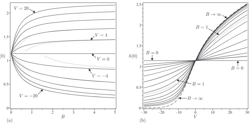
FIG. 3: Film thickness atθ= 0, h(0), plotted as a function (a) ofB forV =−20,−16,−12, . . . , 20 (solid lines) together with the asymptotic solutions in the limitsB→0+

andB → ∞in the casesV =−4 and 4 (dotted lines), and (b) ofV forB = 0 andB= 10n

(n=−1.5,−1.25,−1, . . . , 1.5) (solid lines) together with the asymptotic solutions in the limitsV →0,V → ∞andV → −∞in the caseB = 1 (dotted lines)

and the leading order asymptotic solution in the limitB→ ∞(dashed line), whenQ=−1/2.

range of values ofV and ofV for a range of values of B, respectively. In particular, Figures

2 and 3 illustrate thathis a monotonically increasing (decreasing) function of B for positive

(negative) V, and a monotonically increasing function of V. In addition, Figure 3 shows

good agreement with the asymptotic results forh obtained subsequently.

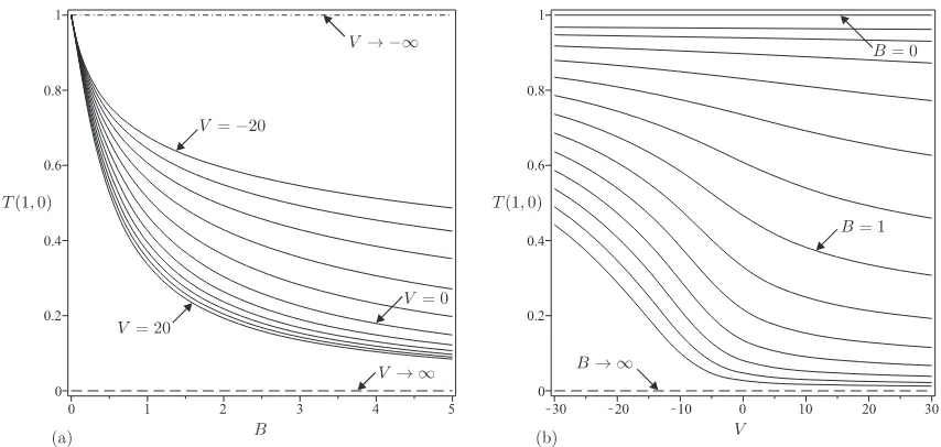
Figure 4 shows the free-surface temperature at θ = 0, T(1,0), plotted as a function of

B for a range of values of V and of V for a range of values of B. Taken together with the

results forhshown in Figures 2 and 3, Figure 4 illustrates that the free-surface temperature,

T(1, θ), is a monotonically decreasing function of bothB and V.

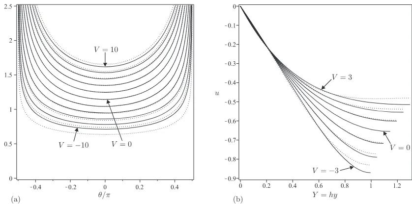
Figure 5 shows the velocity u plotted as a function of Y = hy for a range of values of θ

for both a negative and a positive value ofV, and Figure 6 shows the free-surface velocity at

θ = 0, u(1,0), plotted as a function of B for a range of values of V and of V for a range of

values of B. In particular, Figure 5 shows that the velocity profiles for non-zero values of V

are, in general, quite different from the familiar semi-parabolic profile (25) in the constant

FIG. 4: Free-surface temperature atθ= 0, T(1,0), plotted as a function (a) ofB forV =−20,−16,−12, . . . , 20 (solid lines) together with the leading order asymptotic solution in the limitV → ∞(i.e. T(1,0) = 0) (dashed line) and the leading order asymptotic solution in the limitV → −∞(i.e.T(1,0) = 1)

(dash-dotted line), and (b) of V forB = 0 andB= 10n _(n=

−1.5,−1.25,−1, . . . , 1.5) (solid lines) together with the leading order asymptotic solution in the limitB→ ∞(i.e.T(1,0) = 0) (dashed line),

when Q=−1/2.

FIG. 5: Velocityuplotted as a function ofY =hyforθ= 0,π/64,π/32, . . . , 31π/64 in the cases (a) V =−5 and (b)V = 5, whenQ=−1/2 andB= 1.

of the cylinder.

Figure 8 shows the load M plotted as a function ofB for a range of values ofV and ofV

FIG. 6: Free-surface velocity atθ= 0,u(1,0), plotted as a function (a) ofB forV =−10,−8,−6, . . . , 10 (solid lines) together with the asymptotic solutions in the limits B→0+ _andB

→ ∞in the casesV =−2 and 2 (dotted lines) and the leading order asymptotic solution in the limitV → ∞(i.e.u(1,0) = 0) (dashed

line), and (b) ofV forB= 0 andB = 10n

(n=−1.5,−1.25,−1, . . . , 1) (solid lines) together with the asymptotic solutions in the limitsV →0,V → ∞andV → −∞in the caseB = 10−0.5

≃0.3162 (dotted lines) and the leading order asymptotic solution in the limitB→ ∞(dashed line), whenQ=−1/2.

(decreasing) function ofB for positive (negative)V, and a monotonically increasing function

ofV. In addition, Figure 8 shows good agreement with the asymptotic results forM obtained

subsequently.

In order to obtain a complete understanding of the influence of varying B and V, in

the following Subsections V A–V E we analyse the behaviour in the asymptotic limits of

weak heat transfer at the free surface, B _→ 0+_{, strong heat transfer at the free surface,}

B _{→ ∞}, weak thermoviscosity, V _→0, strong positive thermoviscosity, V _{→ ∞}, and strong

negative thermoviscosity, V _{→ −∞}, respectively. In addition, in the Appendix we analyse

the distinguished limit of strong thermoviscosity and weak heat transfer, _|V_{| → ∞} and

B _→ 0+ _{with BV =O(1), in which, although the variation in temperature across the fluid}

FIG. 7: Typical streamlines of the flow on the right-hand side of the cylinder plotted for ψ= 0 (the cylinder),Q/5, 2Q/5, 3Q/5, 4Q/5 andQ(the free surface) whenQ=−1/2,B= 1 andV = 1.

FIG. 8: LoadM plotted as a function (a) ofB forV =−20,−16,−12, . . . , 20 (solid lines) together with the asymptotic solutions in the limitsB→0+ _andB

→ ∞in the casesV =−4 and 4 (dotted lines), and (b) ofV forB= 0 andB = 10n

(n=−1.5,−1.25,−1, . . . , 1.5) (solid lines) together with the asymptotic solutions in the limitsV →0,V → ∞andV → −∞in the caseB = 1 (dotted lines) and the leading order

A. The limit of weak heat transfer B_→0+

At leading order in the limit of weak heat transfer at the free surface, B _→0+_{, the free}

surface is insulated (i.e. Ty = 0 at y= 1) and, as already discussed in Section IV, the fluid

film is isothermal with constant temperature T _≡ 1, viscosity µ _≡ 1 and fluidity f _≡ 1.

Hence the leading-order solutions forh, uand M are simply the isothermal solutionsh0, u0

and M0 given by (24), (25) and (28), respectively.

The effect of variations in B first appear at O(B), to which order the solutions for h, T,

u and M are given by

h =h0+

BV h2 0

12 +O(B

2_{), (38)}

T = 1₋Bh0y+

B2₍₁₂

−V)h2 0y

12 +O(B

3

), (39)

u=u0−

BV h3 0cosθ

12 (4y

2

−7y+ 2)y+O(B2_{) (40)}

and

M =M0+C1Q2/3BV +O(B2), (41)

where the numerical coefficient C1 is given by

C1 =

1 6

Z π/2

0

3 cosθ

2/3

dθ = π

2

21/3₃5/6_Γ 2 3

3 =

C0

4_×31/6 ≃1.2629. (42)

Note that the solutions (38)–(41) are valid for a general viscosity model satisfying µ = 1

and dµ/dT =₋V when T = 1 to the order shown (but not to higher orders). The solution

(39) shows that the effect of weak heat transfer at the free surface is to decrease T slightly

from its constant isothermal value T _≡ 1 throughout the fluid film. Thus for positive

(negative) thermoviscosityV >0 (V <0) the viscosity is slightly increased (decreased) from

its constant isothermal valueµ_≡1, and determining the sign ofu1 shows that the magnitude

of the velocity is slightly increased (decreased) from its value in the isothermal case when

0< y <(7₋√17)/8_≃0.3596 and slightly decreased (increased) when (7₋√17)/8< y _≤1,

(increased) and hence that the film thickness (and hence the load) is slightly increased

(decreased) everywhere in order to accommodate the fixed volume flux of fluid.

B. The limit of strong heat transfer B_{→ ∞}

At leading order in the limit of strong heat transfer at the free surface, B _{→ ∞}, the free

surface is at the same uniform temperature as the atmosphere (i.e.T = 0 at y= 1) and the

fluid film has non-constant temperature T = ˆT = 1₋y and viscosity µ = ˆµ = µ( ˆT). As

Duffy and Wilson45 _{showed, the leading-order solutions foruand f, denoted by ˆuand ˆf, are}

given by

ˆ

u=₋hˆ2_cosθ

Z 1

ˆ

T

T

µ(T)dT (43)

and (21), respectively, where ˆh denotes the leading-order solution for h. Closed-form

ex-pressions for ˆf for linear, exponential and Eyring viscosity models are described in detail by

Wilson and Duffy25_{. Since ˆf is a constant (and not a function of θ as, in general, f is) the}

leading-order solutions forh and M, the latter denoted by ˆM, are simply given by

ˆ

h= h0 ˆ

f1/3 =

− _ˆ3Q

fcosθ

1/3

, Mˆ = M0 ˆ

f1/3 =C0

|Q_|

ˆ

f

1/3

, (44)

whereh0 andM0are the solutions forhandM of the corresponding isothermal problem with

the same flux given by (24) and (28) in which the constant C0 is again given by (29). Thus,

rather remarkably, for a general viscosity model the film thickness and the load (butnotthe

temperature or the velocity) at leading order in the limit of strong heat transfer are simply

re-scaled versions of their values for the corresponding isothermal problem with the same

flux. In particular, this means that for positive (negative) thermoviscosity the leading-order

film thickness and load are increased (decreased) from their values for the corresponding

isothermal problem with the same flux. Furthermore, in this limit_{V ∼}V, and so the leading

order expressions for µ, u, ψ and f are simply given by (30), (32), (33) and (34) with _V

Note that the re-scaling (44) differs from that proposed by Duffy and Wilson45_{. In general,}

the leading-order solutions forh,QandM in the limit of strong heat transfer, denoted by ˆh,

ˆ

Qand ˆM, are given simply by ˆh= ˆf−m_h

0, ˆQ= ˆf1−3mQ0, and ˆM = ˆf−mM0 forany non-zero

value of m, where h0 andM0 are the solutions for h andM of the corresponding isothermal

problem with flux Q0. Thus at leading order in the limit of strong heat transfer, the film

thickness and the load are simply re-scaled versions of their values for the corresponding

isothermal problem with the appropriate flux. The present scaling (44) corresponds to the

choice m = 1/3 and is simply the special case in which the flux remains unscaled. The

scaling proposed by Duffy and Wilson45 _{corresponds to the choice m = 1/2, who showed}

that this the only possible choice for the corresponding problem of non-isothermal flow on a

uniformly rotatingcylinder at leading order in the limit of strong heat transfer, but failed to

notice that there is no restriction on the value ofmfor the present problem of non-isothermal

flow on astationary cylinder.

As might have been anticipated, this simple re-scaling property does not extend to higher

orders. Specifically, extending the analysis to O(1/B2_{) the solutions for h, T, u and M are}

given by

h= ˆh₋(V + 3) ˆf −3

3 ˆf B +O

1

B2

, (45)

T = ˆT + y

Bˆh +

(Vfˆ₋3)y

3 ˆf B3ˆ_h2 +O

1

B3

, (46)

u= ˆu₋hˆcosθ

3 ˆf BV

6(V ₋1)

V −(2V + 1) ˆf

+

6[1₋V(1₋y)]

V + [1 +V(1−y)(2−3y)] ˆf

exp(₋V y) +O 1 B2 (47) and

M = ˆM ₋

πh(V + 3) ˆf ₋3i

3 ˆf B +O

1

B2

. (48)

The solution (46) shows that the effect of large-but-finite heat transfer at the free surface is

FIG. 9: (a) Film thicknesshplotted as a function ofθ/π forV =−10,−8,−6, . . . , 10 (solid lines), and (b) velocityuat θ= 0 plotted as a function ofY =hyforV =−3,−2,−1, . . . , 3 (solid lines), together with the corresponding asymptotic solutions in the limitV →0 (dotted lines), whenQ=−1/2 andB= 1.

Thus for positive (negative) thermoviscosityV >0 (V <0) the viscosity is slightly decreased

(increased) from its leading-order value µ= ˆµ with the net effect that the film thickness is

slightly decreased (increased) uniformly in order to accommodate the fixed volume flux of

fluid, and hence that the load is slightly decreased (increased).

C. The limit of weak thermoviscosity V _→0

As already discussed in Section IV, at leading order in the limit of weak thermoviscosity,

V _→0, the fluid film has non-constant temperatureT _6≡1 but constant viscosityµ_≡1 and

fluidity f _≡1. From (16) and (17) the solution forh is given by

h=h0+

BV h2 0

12(1 +Bh0)

+O(V2_{), (49)}

and hence from (11), (12) and (18) the solutions for T,u and M are given by

T = 1₋ Bh0y 1 +Bh0 −

B2_{V h}2 0y

12(1 +Bh0)3

+O(V2), (50)

u=u0−

BV h3 0cosθ

12(1 +Bh0)

(4y2

FIG. 10: (a) Film thicknesshplotted as a function ofθ/π forV = 7.5, 15, 22.5, . . . , 60 (solid lines), and (b) velocityuatθ= 0 plotted as a function ofY =hyforV = 4, 8, 12, ..., 40 (solid lines), together with

the corresponding asymptotic solutions in the limitV → ∞(dotted lines), whenQ=−1/2 andB= 1.

and

M =M0+

Q2/3_BV

2_×31/3

Z π/2

0

dθ

(cosθ)2/3_{+B(3|Q|cosθ)}1/3 +O(V 2

), (52)

whereh0,u0 and M0 are the isothermal solutions given by (24), (25) and (28), respectively.

Note that the solutions (49)–(52) are valid for a general viscosity model satisfying µ = 1

and dµ/dT =₋V when T = 1 to the order shown (but not to higher orders). The solutions

in this limit are similar to those in the limit B _→0+ _{described in Subsection V A and have}

a similar physical interpretation. This behaviour is illustrated in Figure 9 which shows the

film thicknesshplotted as a function ofθ/π and the velocity uatθ = 0 plotted as a function

of Y =hy for a range of values ofV near V = 0.

D. The limit of strong positive thermoviscosity V _{→ ∞}

In the limit of strong positive thermoviscosity, V _{→ ∞}, from (16) and (17) the solution

forh is given by

h=h0

V

3 1/3

− 1 3B +O

1

V1/3

and hence from (11), (12) and (18) the solutions for T,u and M are given by

T = 1₋y+ y

Bh0

3

V

1/3

− _3B2y2_h2 0

3

V

2/3 +O 1 V , (54)

u=₋h

2 0cosθ

3

3

V

1/3

[1₋exp(₋V y)]

−h0₉cos_B θ

3

V

2/3

[1₋(1 + 3V y) exp(₋V y)] +O

1 V (55) and

M =M0

V

3 1/3

− ₃π_B +O

1

V1/3

, (56)

whereh0andM0are the isothermal solutions forhandM given by (24) and (28), respectively.

In particular, these solutions show that at leading order in the limit of strong positive

thermoviscosity the temperature is given by T = 1₋y and the viscosity µ = exp(V y) is

exponentially large outside a narrow boundary layer of widthO(1/V)_≪1 near the cylinder

y = 0, resulting in a slow “plug flow” with a uniform (i.e. independent of y) velocity of

O(V−1/3_{) ≪1 outside the boundary layer and a large film thickness of O(V}1/3_{) ≫1. This}

behaviour is illustrated in Figure 10 which shows the film thickness h plotted as a function

of θ/π and the velocity u at θ = 0 plotted as a function of Y = hy for a range of positive

values ofV.

E. The limit of strong negative thermoviscosity V _{→ −∞}

In the limit of strong negative thermoviscosity, V _{→ −∞}, from (16) and (17) the solution

for h is given by

h= 1

B(₋V)log

QB3_V3

2 cosθ

+O

log(₋V)2

V2

, (57)

and hence from (11), (12) and (18) the solutions for T,u and M are given by

T = 1₋ y

(₋V)log

QB3_V3

2 cosθ

+O

log(₋V)

V2

FIG. 11: (a) Film thicknesshplotted as a function ofθ/π forV =−30,−60,−90, . . . ,−180 (solid lines), and (b) velocityuatθ= 0 plotted as a function ofY =hyalso forV =−30,−60,−90, . . . ,−180 (solid

lines), together with the corresponding asymptotic solutions in the limit V → −∞(dotted lines), when Q=−1/2 andB= 1.

u=₋cosθ

B2_V2

QB3_V3

2 cosθ

y log

QB3_V3

2 cosθ

(1₋y) + 1

−log

QB3_V3

2 cosθ

−1

+O(log(₋V)) (59)

and

M = πlog(|Q|B

3₍

−V)3₎

B(₋V) +O

log(₋V)2

V2

. (60)

In particular, these solutions show that at leading order in the limit of strong negative

thermoviscosity the temperature is given by T = 1 and the viscosity

µ=

2 cosθ QB3_V3

y

(61)

decreases from O(1) at the cylinder y= 0 to O((₋V)−3₎

≪1 at the free surface y = 1 and

that the velocity increases from zero at the cylinder (where there is a narrow boundary layer

of width O(1/log(₋V)) _≪ 1) to O(₋V) _≫ 1 at the free surface (where there is another

narrow boundary layer also of widthO(1/log(₋V))_≪1), resulting in a small film thickness

of O(log(₋V)/(₋V)) _≪1. This behaviour is illustrated in Figure 11 which shows the film

thickness h plotted as a function of θ/π and the velocity u atθ = 0 plotted as a function of

VI. CONCLUSIONS

In the present work we obtained a comprehensive description of the two-dimensional

steady gravity-driven flow with prescribed volume flux of a thin film of Newtonian fluid with

temperature-dependent viscosity on a heated or cooled stationary horizontal cylinder. In

particular, we showed that for the exponential viscosity model (7) the effect of increasing

B depends on the sign of V. When the cylinder is hotter than the surrounding atmosphere

(i.e. when V > 0) the effect of increasing B is to decrease the average temperature and

so to increase the average viscosity and hence reduce the average velocity within the film,

with the net effect that the film thickness (and hence the total fluid load on the cylinder) is

increased to maintain the fixed volume flux of fluid. When the cylinder is colder than the

surrounding atmosphere (i.e. when V < 0) the opposite occurs. Similarly, we showed that

the effect of increasingV is always to increase the film thickness and hence the load. In order

to obtain a complete understanding of the influence of varying B and V, we also analysed

the behaviour in the asymptotic limits of weak heat transfer,B _→0+_{, strong heat transfer,}

B _{→ ∞}, weak thermoviscosity, V _→0, strong positive thermoviscosity, V _{→ ∞}, and strong

negative thermoviscosity, V _{→ −∞}, as well as (in the Appendix) in the distinguished limit

of strong thermoviscosity and weak heat transfer, _|V_{| → ∞} and B _→0+ _{with BV =O(1).}

The asymptotic analysis in the limits B _→ 0+ _{and B}

→ ∞ revealed that increasing B

from zero to infinity changes the film thickness everywhere (and hence the load, but not the

temperature or the velocity) by a constant factor of ˆf−1/3_{, where ˆf is given by (21), which}

depends only on the specific viscosity model considered. The asymptotic analysis in the

limits V _→0, V _{→ ∞} and V _{→ −∞} revealed that for the exponential viscosity model (7)

the behaviour of the solution for large positive thermoviscosity is very different from that

for large negative thermoviscosity, and that both are very different from that in the constant

viscosity caseV = 0. Specifically, in the limit V _{→ ∞}the viscosity is exponentially large of

O(exp(V))_≫1 and the velocity is small and uniform (i.e. independent ofy) ofO(V−1/3₎

outside a narrow boundary layer of widthO(1/V)_≪1 near the cylinder, leading to a large

film thickness ofO(V1/3_{)≫1, while in the limitV → −∞the viscosity decreases fromO(1)}

at the cylinder to O((₋V)−3_{) ≪ 1 at the free surface and the velocity increases from zero}

at the cylinder to a large value of O(₋V) _≫ 1 at the free surface, leading to a small film

thickness ofO(log(₋V)/(₋V))_≪ 1.

APPENDIX A: DISTINGUISHED LIMIT OF STRONG THERMOVISCOSITY

AND WEAK HEAT TRANSFER _|V_{| → ∞} AND B _→0+ _{WITHVˆ =BV =O(1)}

Another interesting case also worth considering is the distinguished limit discussed by

Wilson and Duffy26 _{of strong thermoviscosity, |V| → ∞, and weak heat transfer at the free}

surface,B _→0+_{, such that ˆV =BV =O(1), in which, although the variation in temperature}

across the fluid film is small, specifically T = 1₋Bhy+O(B2_{), thermoviscosity effects still}

enter the problem at leading order, i.e. the variation in viscosity across the fluid film is still

O(1). Note that in this limit theeffective thermoviscosity number, ˆV =BV, defined in terms

of dimensional quantities by

ˆ

V = λ(T0−T∞)ǫaαth

µ0kth

, (A1)

and not the previously defined thermoviscosity number, V, is the appropriate

non-dimensional measure of thermoviscosity effects. In the particular case of the exponential

viscosity model (30) in this limit _{V ∼} V hˆ and so the leading order expressions for µ, u, ψ

and f are simply given by (30), (32)–(34) with _V replaced by ˆV h, respectively.

Note that, in an analogous way to being able to remove B explicitly from the general

mathematical problem by rescaling appropriately (discussed in Section III), in this case

we could remove ˆV explicitly from the mathematical problem by rescaling h, u, ψ and Q

appropriately; however, since this again obscures the physical interpretation of the results

obtained we retain ˆV explicitly in what follows.

the corresponding results in the limitB _→0 given in Subsection V A, namely (38), (40) and

(41), with BV replaced by ˆV, and hence have the same physical interpretation.

In the limit of strong positive thermoviscosity, ˆV _{→ ∞}, the solutions for h,u and M are

given by

h= ₋QVˆ cosθ

!1/2 + 1

ˆ

V +O

1 ˆ

V5/2

, (A2)

u=₋cosθ ˆ

V −

QVˆ

cosθ

!1/2 



1₋exp 

− −

QVˆ3

cosθ

!1/2

y      +O 1 ˆ V2 (A3) and

M = ˆC_|Q_|Vˆ1/2+ π ˆ

V +O

1 ˆ

V5/2

, (A4)

in which the numerical coefficient ˆC is given by

ˆ

C = 2 Z π/2

0

1 cosθ

1/2

dθ = 2√2 K

1 √ 2

≃5.2441, (A5)

where K(k) is the complete elliptic integral of the first kind with modulus k defined by

K(k) = Z 1

0

dx

√

1₋x2√_1−k2_x2 (A6)

(see, for example, Gradshteyn and Ryzhik46_{). These solutions differ from the corresponding}

results in the limit V _{→ ∞} given in Subsection V D, namely (53), (55) and (56), but have

a qualitatively similar physical interpretation. In particular, these solutions show that at

leading order in the limit of strong positive thermoviscosity the viscosity

µ= exp 

 −

QVˆ3

cosθ

!1/2

y



 (A7)

is exponentially large outside a narrow boundary layer of width O( ˆV−3/2_{) ≪ 1 near the}

cylindery= 0, resulting in a slow “plug flow” with a uniform (i.e. independent ofy) velocity

of O( ˆV−1/2₎

≪1 outside the boundary layer and a large film thickness of O( ˆV1/2₎

≫1.

In the limit of strong negative thermoviscosity, ˆV _{→ −∞}, the solutions for h, u and M

are given by

h= 1

(₋Vˆ)log

QVˆ3

2 cosθ

!

+O log((−Vˆ)

6₎

ˆ

V4

!

u=₋cosθ ˆ

V2

"

QVˆ3

2 cosθ

!y(

log QVˆ

3

2 cosθ

!

(1₋y) + 1 )

−log QVˆ

3

2 cosθ

!

−1 #

+O log((−Vˆ)

6₎

ˆ

V2

!

(A9)

and

M = πlog(|Q|(−Vˆ)

3₎

(₋Vˆ) +O

log((₋Vˆ)6₎

ˆ

V4

!

. (A10)

At leading (but not higher) order these solutions coincide with the corresponding results in

the limitV _{→ −∞}given in Subsection V E, namely (57), (59) and (60), and hence have the

same physical interpretation.

ACKNOWLEDGEMENTS

The first author (GAL) gratefully acknowledges the financial support of the United

King-dom Engineering and Physical Sciences Research Council (EPSRC) via a Doctoral Training

Account (DTA) research studentship. This work was completed while the second author

(SKW) was a Visiting Fellow in the Department of Mechanical and Aerospace Engineering

in the School of Engineering and Applied Science at Princeton University, USA.

1 _{W. Nusselt, “Die Oberfl¨achenkondensation des Wasserdampfes,” Z. Vereines deutscher}

Inge-nieure60, 541–546 (1916).

2 _{W. Nusselt, “Die Oberfl¨achenkondensation des Wasserdampfes,” Z. Vereines deutscher}

Inge-nieure60, 569–575 (1916).

3 _{E. M. Sparrow and J. L. Gregg, “Laminar condensation heat transfer on a horizontal cylinder,”}

J. Heat Transfer 81, 291–296 (1959).

4 _{A. A. Nicol, Z. L. Aidoun, R. J. Gribben, and G. Wilks, “Heat transfer in the presence of}

condensate drainage,” Int. J. Multiphase Flow 14, 349–359 (1988).

5 _{J.-J. Shu and G. Wilks, “Heat transfer in the flow of a cold, two-dimensional draining sheet over}

a hot, horizontal cylinder,” Eur. J. Mech. B. Fluids28, 185–190 (2009).

6 _{I. G. Shekriladze and V. I. Gomelauri, “Theoretical study of laminar film condensation of flowing}

7 _{T. Fujii, H. Uehara, and C. Kurata, “Laminar filmwise condensation of flowing vapour on a}

horizontal cylinder,” Int. J. Heat Mass Transfer15, 235–246 (1972).

8 _{J. W. Rose, “Effect of pressure gradient in forced convection film condensation on a horizontal}

tube,” Int. J. Heat Mass Transfer 27, 39–47 (1984).

9 _{C.-K. Chen and Y.-T. Lin, “Laminar film condensation from a downward-flowing steam-air}

mixture onto a horizontal circular tube,” Appl. Math. Modell.33, 1944–1956 (2009).

10 _{P. K. Sarma, B. Vijayalakshmi, F. Mayinger, and S. Kakac, “Turbulent film condensation on}

a horizontal tube with external flow of pure vapors,” Int. J. Heat Mass Transfer 41, 537–545

(1998).

11 _{S.-A. Yang and Y.-T. Lin, “Turbulent film condensation on a non-isothermal horizontal tube –}

effect of eddy diffusivity,” Appl. Math. Modell. 29, 1149–1163 (2005).

12 _{S.-A. Yang and C.-H. Hsu, “Free- and forced-convection film condensation from a horizontal}

elliptic tube with a vertical plate and a horizontal [sic] tube as special cases,” Int. J. Heat Fluid Flow 18, 567–574 (1997).

13 _{Y.-T. Lin and S.-A. Yang, “Turbulent film condensation on a horizontal elliptical tube,” Heat}

Mass Transfer41, 495–502 (2005).

14 _{B. Reisfeld and S. G. Bankoff, “Non-isothermal flow of a liquid film on a horizontal cylinder,”}

J. Fluid Mech. 236, 167–196 (1992).

15 _{A. T. Conlisk and J. Mao, “Nonisothermal absorption on a horizontal cylindrical tube – 1. The}

film flow,” Chem. Eng. Sci. 51, 1275–1285 (1996).

16 _{D. Goussis and R. E. Kelly, “Effects of viscosity variation on the stability of film flow down heated}

or cooled inclined surfaces: Long-wavelength analysis,” Phys. Fluids28, 3207–3214 (1985).

17 _{D. A. Goussis and R. E. Kelly, “Effects of viscosity variation on the stability of a liquid film flow}

down heated or cooled inclined surfaces: Finite wavelength analysis,” Phys. Fluids30, 974–982 (1987).

18 _{C.-C. Hwang and C.-I. Weng, “Non-linear stability analysis of film flow down a heated or cooled}

inclined plane with viscosity variation,” Int. J. Heat Mass Transfer 31, 1775–1784 (1988).

19 _{B. Reisfeld and S. G. Bankoff, “Nonlinear stability of a heated thin liquid film with variable}

viscosity,” Phys. Fluids A 2, 2066–2067 (1990).

20 _{M.-C. Wu and C.-C. Hwang, “Nonlinear theory of film rupture with viscosity variation,” Int.}

Comm. Heat Mass Transfer18, 705–713 (1991).

21 _{R. Selak and G. Lebon, “B´enard-Marangoni thermoconvective instability in presence of a}

temperature-dependent viscosity,” J. Phys. II France 3, 1185–1199 (1993).

22 _{D. Bercovici, “A theoretical model of cooling viscous gravity currents with}

temperature-dependent viscosity,” Geophys. Res. Lett. 21, 1177–1180 (1994).

23 _{N. J. Balmforth and R. V. Craster, “Dynamics of cooling domes of viscoplastic fluid,” J. Fluid}

Mech.422, 225–248 (2000).

24 _{Yu. O. Kabova and V. V. Kuznetsov, “Downward flow of a nonisothermal thin liquid film with}

25 _{S. K. Wilson and B. R. Duffy, “On the gravity-driven draining of a rivulet of fluid with}

temperature-dependent viscosity down a uniformly heated or cooled substrate,” J. Eng. Math.

42, 359–372 (2002).

26 _{S. K. Wilson and B. R. Duffy, “Strong temperature-dependent-viscosity effects on a rivulet}

draining down a uniformly heated or cooled slowly varying substrate,” Phys. Fluids15, 827–840 (2003).

27 _{B. R. Duffy and S. K. Wilson, “A rivulet of perfectly wetting fluid with temperature-dependent}

viscosity draining down a uniformly heated or cooled slowly varying substrate,” Phys. Fluids

15, 3236–3239 (2003).

28 _{A. Sansom, J. R. King, and D. S. Riley, “Degenerate-diffusion models for the spreading of thin}

non-isothermal gravity currents,” J. Eng. Math.48, 43–68 (2004).

29 _{R. Usha, R. Ravindran, and B. Uma, “Dynamics and stability of a thin liquid film on a heated}

rotating disk film with variable viscosity,” Phys. Fluids 17, 102103 (2005).

30 _{L. Wu, “Spin coating of thin liquid films on an axisymmetrically heated disk,” Phys. Fluids18,}

063602 (2006).

31 _{C.-K. Lin, C.-C. Hwang, and T.-C. Ke, “Three-dimensional nonlinear rupture theory of thin}

liquid films on a cylinder,” J. Colloid Interface Sci. 256, 480–482 (2002).

32 _{A. A. King, L. J. Cummings, S. Naire, and O. E. Jensen, “Liquid film dynamics in horizontal}

and tilted tubes: Dry spots and sliding drops,” Phys. Fluids19, 042102 (2007).

33 _{L. R. Band, D. S. Riley, P. C. Matthews, J. M. Oliver, and S. L. Waters, “Annular thin-film}

flows driven by azimuthal variations in interfacial tension,” Q. J. Mech. Appl. Math.62, 403–430

(2009).

34 _{O. Haimovich and A. Oron, “Nonlinear dynamics of a thin liquid film on an axially oscillating}

cylindrical surface,” Phys. Fluids22, 032101 (2010).

35 _{H. K. Moffatt, “Behaviour of a viscous film on the outer surface of a rotating cylinder,” J. M´ec.}

16, 651–673 (1977).

36 _{V. V. Pukhnachev, “Motion of a liquid film on the surface of a rotating cylinder in a gravitational}

field,” J. Appl. Mech. Tech. Phys.18, 344–351 (1977).

37 _{R. E. Johnson, “Steady-state coating flows inside a rotating horizontal cylinder,” J. Fluid Mech.}

190, 321–342 (1988).

38 _{B. R. Duffy and S. K. Wilson, “Thin-film and curtain flows on the outside of a rotating horizontal}

cylinder,” J. Fluid Mech. 394, 29–49 (1999).

39 _{J. Ashmore, A. E. Hosoi, and H. A. Stone, “The effect of surface tension on rimming flows in a}

partially filled rotating cylinder,” J. Fluid Mech. 479, 65–98 (2003).

40 _{M. Villegas-D´ıaz, H. Power, and D. S. Riley, “Analytical and numerical studies of the stability}

of thin-film rimming flow subject to surface shear,” J. Fluid Mech. 541, 317–344 (2005).

41 _{E. S. Benilov, M. S. Benilov, and N. Kopteva, “Steady rimming flows with surface tension,” J.}

Fluid Mech. 597, 91–118 (2008).

a rotating horizontal cylinder: Theory and experiment,” Phys. Fluids17, 072102 (2005).

43 _{M. A. Kelmanson, “On inertial effects in the Moffatt–Pukhnachov coating-flow problem,” J.}

Fluid Mech. 633, 327–353 (2009).

44 _{R. Hunt, “Numerical solution of the free-surface viscous flow on a horizontal rotating elliptical}

cylinder,” Numer. Methods Partial Differential Eq. 24, 1094–1114 (2008).

45 _{B. R. Duffy and S. K. Wilson, “Large-Biot-number non-isothermal flow of a thin film on a}

stationary or rotating cylinder,” Eur. Phys. J. Special Topics 166, 147–150 (2009).

46 _{I. S. Gradshteyn and I. M. Ryzhik, Tables of Integrals, Series and Products, 2nd ed., (Academic}