Architecture of a Network-in-the-Loop Environment
for Characterizing AC Power-System Behavior
Andrew J. Roscoe, Andrew Mackay, Graeme M. Burt,
Member, IEEE
, and J. R. McDonald,
Member, IEEE
Abstract—This paper describes the method by which a large hardware-in-the-loop environment has been realized for three-phase ac power systems. The environment allows an entire laboratory power-network topology (generators, loads, controls, protection devices, and switches) to be placed in the loop of a large power-network simulation. The system is realized by using a real-time power-network simulator, which interacts with the hardware via the indirect control of a large synchronous generator and by measuring currents flowing from its terminals. These measured currents are injected into the simulation via current sources to close the loop. This paper describes the system architecture and, most importantly, the calibration methodologies which have been developed to overcome measurement and loop latencies. In partic-ular, a new “phase advance” calibration removes the requirement to add unwanted components into the simulated network to com-pensate for loop delay. The results of early commissioning exper-iments are demonstrated. The present system performance limits under transient conditions (approximately 0.25 Hz/s and 30 V/s to contain peak phase- and voltage-tracking errors within 5◦and 1%) are defined mainly by the controllability of the synchronous generator.
Index Terms—Calibration, digital control, electric variable measurement, power-system protection, power-system secu-rity, power-system simulation, power-system stability, real-time systems.
NOMENCLATURE
IG Vector of three-phase currents from 80 kVA generator.
IN Vector of three-phase currents flowing into hardware.
Kf Feedforward control gain (normally one) for throttle.
Kϕ Frequency target offset per radian of phase-tracking error.
tC Interface delay time which needs to be calibrated.
VN Vector of three-phase voltages at shared node in hardware.
V∗
N Vector of three-phase voltages at shared node in simulation.
Manuscript received March 9, 2009; revised June 2, 2009. First published June 16, 2009; current version published March 10, 2010. This work was supported in part by Rolls-Royce PLC and in part by the Engineering and Physical Sciences Research Council Supergen Programme.
A. J. Roscoe, G. M. Burt, and J. R. McDonald are with the Rolls-Royce University Technology Centre, Institute for Energy and Environment, Department of Electronic and Electrical Engineering, University of Strath-clyde, G1 1XW Glasgow, U.K. (e-mail: [email protected]; [email protected]; [email protected]).
A. Mackay was with the University of Strathclyde, G1 1XW Glasgow, U.K. He is now with Rolls-Royce PLC, DE24 8BJ Derby, U.K. (e-mail: [email protected]).
Digital Object Identifier 10.1109/TIE.2009.2025242
I. INTRODUCTION
T
HE USE OF hardware-in-the-loop (HIL) digital simula-tion for the testing of power equipment has increased in popularity over recent years. A key enabler of this is the avail-ability of computing power necessary to simulate power sys-tems in real time, with the fidelity required to simulate transient phenomena in power systems. Traditionally, HIL simulation has been used for the testing of secondary power equipment such as protection relays and controllers for machines and converters [1]–[7].A key aspiration, however, is to couple entire electrical net-works in hardware to digital models of other electrical netnet-works running in real time. The hardware network might contain many generators, loads, cables, transmission lines, and transformers. The simulated network might be even more complex or might be a very simple network such as an infinite bus or a large single generator. The construction of such a system allows sections of power systems to be constructed in hardware and coupled to simulations of larger power networks which cannot be implemented in hardware due to constraints of time, cost, and space. The results from experiments performed on such a system have high credibility due to the use of actual hardware and control systems wherever possible. For example, the works of [8]–[11] could be further verified by installing the proposed hardware (several photovoltaic inverters with controllers, diesel generators and/or battery storage, loads, etc.) in the laboratory at the multikilowatt scale and coupling them to a simulation of the distribution grid at a suitable point of common coupling. The proposed hardware network can then be subjected to simulations of grid perturbations, faults, etc., and the desired response is verified. Such a step represents a sensible final test of a prototype power system before deployment in the real world.
Achieving such a goal requires a specialized interface to “transfer” power and maintain the conservation of energy be-tween the simulated network and the hardware network. This interface must emulate the simulated model at the point where the hardware is connected. Generally, a controllable power supply is needed where the current and voltage output can be set. This is known as power HIL (PHIL) simulation.
The characterization of the restrictions for stable PHIL must be highlighted. A key issue is the delay introduced in the inter-face between the digitally simulated network and the physical hardware network. Generally, the minimum delay possible is restricted by the timeframe of the digital simulation. This is generally in the region of 10–100 μs in a dynamic electro-magnetic simulation; for example, the default time frame for
network simulations on the real-time digital simulator (RTDS) [12] system is 50μs.
There are methods for reducing errors caused by the interface delay by adding additional components in simulation to com-pensate for the delay. This may be a transmission line model, using the Bergeron traveling wave method, or a transformer. This is a recommended method for use with the RTDS [13]. However, there are limits to this. The compensating component must have the parameters that will compensate for the delay. If a transmission line is used, the minimum length of the line is restricted by the size of the time delay. Similarly, if a trans-former is used, the minimum reactance of the transtrans-former is restricted. There have been efforts to minimize this restriction. Verma et al. [14] demonstrate a method for utilizing shorter lines to interface the hardware and software. These techniques still require the introduction of additional components into the simulated network. This may not be ideal in certain networks. For example, real marine power systems have low impedance; therefore, adding such artificial components can degrade the accuracy of dynamic studies or fault studies on these networks. Wuet al.propose a solution to the error caused by this time delay by representing the hardware-under-test (HUT) with a linear time-varying first-order system to predict the behavior of the HUT [15]. Results show that this can reduce the error introduced by the delay, although, in the example used, the HUT is a first-order resistor/inductor circuit. This technique may not be as effective for more complex networks with nonlinear components.
Other constraints for PHIL must also be considered such as measurement accuracy and interface dynamics. Ayasun et al.
suggest a system to evaluate the performance of the interface by categorizing parameters required such as latency and mea-surement accuracy [16]. Renet al.[17] highlight the stability issues that become inherent in PHIL simulation and assess the effectiveness of several interfacing techniques, highlighting the strengths and weaknesses of each.
There are few test facilities available that have capabilities of PHIL simulation with primary hardware. The Centre for Advanced Power Systems facility in Florida State University has the capability to test 5 MW machines [18], wind energy systems [19], and drive controllers [20] and run complex all-electric ship models in real time [21] using several RTDS systems in parallel operation.
The University of Newcastle-Upon-Tyne has also reported the capability of PHIL with the development of a 145 kW virtual power system [22].
[image:2.594.310.555.72.245.2]PHIL simulation generally relies on high-powered control-lable sources to interface the hardware and emulate the soft-ware network. A solid-state inverter is typically used, but this requires expensive high-powered components and a custom control system. Depending on the study, it may also need refined voltage or current resolution. The method presented in this paper relies on the control of a synchronous generator as the interface between the hardware and software components of the network (see Section II). This is particularly suited for simulat-ing balanced three-phase systems with low dynamic changes, since hardware capacitive/inductive filters at the interface for improving total harmonic distortion (THD) are not required.
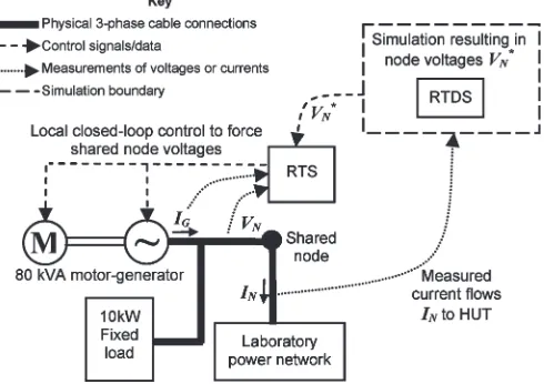
Fig. 1. Closing the loop between simulation and hardware.
In the method described, no artificial components are intro-duced to the simulated network to compensate for the interface delay. Instead, interface delay compensation is dealt with by introducing a new “phase advance” calibration. This technique is not specific to the synchronous generator method described here and could equally be applied to an inverter-based interface. In addition, since the laboratory is a large power network with many devices, substantial care must be taken with all voltage and current measurements to ensure that their amplitude and phase accuracies are acceptable. This paper describes the opti-mized calibration methodologies which have been developed to account for varying performance across many hardware mea-surement channels, including the effects of antialiasing filters and analog-to-digital converter (ADC) skews. These calibra-tions are described in detail in Section III. Section IV follows to describe the control of the synchronous generator. Finally, the performance of the entire PHIL system, when perturbed by dynamic load changes within both simulation and hardware, is demonstrated in Section V. Conclusions and further work opportunities are summarized in Section VI.
II. ARCHITECTUREOVERVIEW ANDPRINCIPLE
This system was originally installed to mimic a generator installation at the multimegawatt scale.
The voltages at the generator/load-bank terminals are driven, as accurately as can be achieved, to match the simulated nodal voltages at the shared node in real time. This causes currents
IN to flow in the laboratory network (HUT). The hardware can consist of cables, switches, impedances, generators (syn-chronous, induction, inverter, etc.), or loads (static resistive, static reactive, induction, etc.). This, in turn, causes frequency, voltage, and power-flow fluctuations in these hardware ele-ments. Microgrid management algorithms which control parts of the laboratory power network may also react by adjusting controls, switches, loads, or generators in real time. The closure of the simulation loop is achieved by measuring the three-phase currentsIN. These three current measurements are then passed back to the simulation, where they are injected at the shared node by using three single-phase current-source elements.
A. Architecture Details
The network simulation is carried out on an RTDS simulator [12], which operates with a 50μs frame time. This uses the RSCAD [23] simulation environment. This simulation resource is two floors distant from the laboratory hardware and the machine controls. The laboratory hardware, including the ma-chine controls for the 80 kVA motor–generator set, is controlled using a real-time-system (RTS) controller [24], which is a multiprocessor VERSA-module Europe (VME) based system, operating at a 2000μs fundamental frame time with ADC sam-pling and digital prefiltering at 666.66μs. The RTS controller can be programmed via MATLAB Simulink (using the Real-Time Workshop extension) which makes it suitable for the rapid prototyping and implementation of novel power-system control and protection schemes [3]. The RTS controller is situated locally to the laboratory hardware, since it has many hardwired instrumentation connections to the hardware. This hybrid use of the RTDS simulator and the RTS controller results in some communication overhead, but allows the different strengths of each of these two devices to be best used.
B. Instrumentation and Communication
The measurement ofVN, which is the voltage at the shared node, is done by using a three-phase voltage transformer (VT). The measurement of the currents IN andIG is done using current transformers (CTs) burdened with suitable resistances. In all cases, shielded treble twisted-pair cable sets are used to bring the signals to the RTS controller (VNandIG) and RTDS simulator(IN), via suitable scaling, isolation, and antialiasing filtering. The measurementIG is not directly required for the HIL system but is used for the feedforward control of the 80 kVA drive, described in Section IV. At the RTS controller and RTDS simulator, the signals are sampled using ADCs. A nontrivial stage is the passing of data from the RTDS simulator to the RTS controller. These data consist of the three-phase voltage set V∗N which the RTDS simulation wishes to force at the shared node. This passing of data is required because the
simulation and control functions have been split between the RTDS simulator and RTS controller.
It was considered to implement this control digitally via an optical link, and this may eventually prove to be a better system due to lower calibration and noise errors. In the present implementation, however, the simulated three-phase voltage set
V∗
N at the shared node in the simulation is simply passed using analog voltages. The signals pass from three digital-to-analog converters (DACs) at the RTDS simulator via a shielded treble twisted-pair cable set to the RTS controller where they are resampled on three unfiltered ADCs.
Comprehensive data logging is carried out using the RTS controller infrastructure. The results of the simulation on the RTDS can also be captured. Matching the two sets of data together after test runs presently requires some degree of man-ual intervention since there is currently no synchronized clock information between the RTS and RTDS data sets.
III. CALIBRATION ANDLOOPLATENCY
Referring to Fig. 1, there are three important latency mech-anisms which need to be understood. These mechmech-anisms are described next. The second and third mechanisms must be carefully accounted for via calibrations.
First, there is an overall loop latency which includes the RTS processing/measurement time, 80 kVA generator response time, and RTDS processing time. The processing loop latency is on the order of 3000–6000 μs, dominated by a time of 112–3 frames for the RTS controller to sample, process, and output its results. This time is of little consequence being on the order of 15% of one cycle at 50 Hz. The signal mea-surement algorithms within the RTS controller average over 112–2 cycles for amplitude and phase measurements and five cycles for measuring frequency, adding up to ∼50 ms to the complete response time. These measurement algorithms have been optimized to minimize noise and ripple in the presence of interference and THD during laboratory experiments, and there is scope to reduce these times for use specifically in the PHIL application. Of most significance is the generator response time to torque and field controls, which dominates the loop latency. The generator response time thus sets limits on the ROCOF rate (hertz per second) and voltage slew rate (volts per second) which can be accurately tracked by the hardware. These limits are demonstrated in Section V.
sensible) if a common filter design is used for each group of three or six channels (voltages, currents, or voltages and currents) since this simplifies the calibration implementation and Fourier/sequence/power-flow analysis. The sets of three or six measurements should also be made on adjacent ADC channels to minimize the timing skew within the sets.
Fortunately, because the timings of the ADC reads are re-peatable on a frame-by-frame basis and because the designs of the antialiasing filters are known, it is possible to calculate and implement calibrations for amplitude and time/phase on all channels. This process has been developed and optimized for the PHIL application, both for accuracy and minimization of computational effort. The steps are as follows.
1) Calculate the amplitude attenuations at the system fre-quency due to antialias filter characteristics and correct each ADC reading by linear multiplication.
2) To account for the relative ADC channel–channel time skews within each set of three (voltages or currents) or six (voltages and currents) readings, the sample sets can be corrected in the time domain by using a second-order interpolation technique optimized from [25], using the most recent three samples. A simpler first-order technique was considered but this introduces small attenuations to the signals which would require correction using addi-tional amplitude calibrations. The interpolation delays the signals by very small amounts in a staggered manner so that all readings appear coherent within each set (but not necessarily between sets). Normally, the maximum relative skews within sets are only on the order of 20μs for sets of three readings or 50μs for sets of six readings, which represent small delays within a 2000 μs frame. Carrying out this correction in the time domain for the sets of three or six readings allows a significant reduction in the subsequent computational effort when carrying out sequence and power-flow analysis, by reducing the number of trigonometric functions required for those stages. On each channel, the procedure calculates
k0=y−1 k1=(y0−y−2)
2 k2=
(y0+y−2)
2 −y−1
where y0, y−1, and y−2 are the most recent, previous, and oldest samples, respectively. Then, the reading can be made coherent with other channels by calculating
x= 1−tTLag
S y=k2x
2+k 1x+k0
where tLag for each channel is the small required time offset to bring each channel into coherence with all the others in the set andTsis the frame time.
3) Carry out Fourier, sequence, and power-flow analyses, using algorithms optimized for accuracy and computa-tional speed, using minimal calculations of trigonometric functions by careful reuse of such calculations [26], [27]. 4) Apply overall gross phase lag corrections due to antialias filter lags and overall relative ADC timings across all ADC cards at the system frequency. These lags can be
significant (up to 45◦ for an antialias filter and 800μs for overall ADC channel skews across all channels). The gross phase lags are applied by linear addition (in the frequency domain) to the calculated phases of the voltages, currents, and sequences. This finally brings all the results from all the measurement sets to a point where the signal phases can be compared accurately.
The VT, CT, instrumentation circuits, and antialias filters are designed and constructed using fixed 1% tolerance parts throughout (two-pole Sallen–Key filter circuits in the unity-gain configuration proving to be highly effective and repeatable), with overall amplitude accuracy of this order and phase accu-racy of approximately 1◦. Thus far, this approach has allowed all calibration factors to be calculated theoretically and has avoided the necessity for many time-consuming measurement-based calibrations. The accuracy of the system can be checked against a calibrated third-party device at intervals to validate the performance.
An important item to note is that, if the RTS controller calibrations are successfully implemented, the RTS controller acquires coherent measurements of V∗N and VN (and IG). Thus, the closed-loop nature of the 80 kVA generator control by the RTS controller means that (at steady state) the voltagesVN can be held exactly in synchronism with the target voltage set
V∗
N provided by the RTDS simulator, to within approximately 1% amplitude and 1◦phase.
The third latency mechanism involves the processing delay (interface delay) tC within the hardware–RTDS–RTS part of the loop. This delay is small, but it must be accounted for; otherwise, the measured currentsIN will lag behind those that should ideally arise given the simulated target voltagesV∗N.
As previously mentioned, the time taken to read the values ofV∗N at the RTS controller does not contribute to this delay, since theV∗N andVN voltages can be brought to coherence. The processing delay tC is thus given by the time taken for the RTDS simulator to measure IN, process the simulation, and output the result. Propagation delays through the twisted pair lines will account for only a few microseconds (0.33 μs for 100 m in free space). The delay is therefore dominated by the CT phase lag (which might give 55 μs for a 1◦ lag at 50 Hz), RTDS antialiasing filter (a 1 kHz single-pole low-pass filter was used, giving a 159 μs lag at 50 Hz), RTDS ADC sample time, processing time (at a 50μs frame time), and DAC output time.
Thus, tC might be expected to be in the region of 250– 500 μs, bearing in mind that, within the RTDS simulator, the network simulation, controls, ADC reading, and DAC outputs are handled by different processors, and a single 50μs delay is incurred for each processor–processor communication. This adds several multiples of 50μs to the nominal 50μs frame time. The overall delay can be measured and calibrated by adjusting
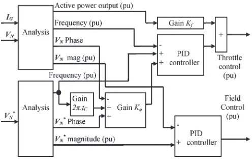
Fig. 2. 80-kVA generator throttle and field controls.
this procedure,tC has been found to be 425μs, at the higher end of the expected range. During the calibration, 20 kVA was flowing at 400 V line–line (29 A per phase) at a power factor (PF) of 0.93 (lagging). The average power angle of the measured power flows on both the RTS controller and RTDS simulator was adjusted (viatC) to be−20.7±0.2◦.
Note that, if the loop latency was not accounted for, the power angles perceived at the RTDS and RTS would then be divergent by atan(425 μs/(1/50 Hz)) = 1.2◦ even at steady state during all PHIL scenarios, unless artificial components were added into the RTDS simulation. During calibration, the peak noise on individual sampled RTS/RTDS power angle measurements was up to ±0.6◦ despite the careful use of screened twisted-pair cables and differential inputs throughout the instrumentation/measurement circuits. The noise on the power angle measurement occurs partly because the currentIN can be measured up to 125 A; therefore, a 29 A flow represents only 23% of the full-scale range.
IV. CONTROL OFFORCEDVOLTAGESOURCE (80-kVA GENERATOR)
A critical capability, handled by the RTS controller, is the ability to match the actual voltages VN to the simulated voltages V∗N in real time, both in amplitude and phase. The active control of the phase of a synchronous generator is un-conventional and is achieved here by using fast-acting controls for the armature current of the motor which drives the 80 kVA generator. To create the phase-locking control system, an ex-isting application which implemented a droopless frequency and voltage control via proportional–integral–differential (PID) control loops has been modified and augmented. The generator frequency/phase is manipulated with the throttle control, while the voltage magnitude is manipulated with the field control. Fig. 2 shows a simplified diagram of the control scheme. The error signal for the field PID controller is simply the difference between the positive sequence magnitudes ofV∗N andVN.
The error signal to the throttle PID controller is more com-plex, consisting of two main terms. The first is the differ-ence between the frequencies of V∗N and VN, which tends to bring the frequency of the generator toward that of the simulation. The second error term consists of a gainKϕtimes
Fig. 3. Example of a simple simulation on the RTDS.
the difference between the phases ofV∗N andVN. This error term tends to bring the generator terminal voltages into phase lock with the desired simulation voltages V∗N. The value of
Kϕ has been set by empirical tuning to0.2/π, equating to a maximum 5 Hz offset for a 90◦ phase-lock error. The com-pensation parameter tC is described in Section III. The use of a throttle feedforward control term Kf(= 1) significantly improves the phase/frequency response of the generator when subjected to step changes in load. The improvement occurs because a change in power flow can be measured within 112–2 cycles, whereas any resulting change in frequency occurs more slowly, as an integral response to power imbalance, in-versely proportional to the inertia of the generator and HUT hardware.
Subtle extra features of the control are an additional small-frequency offset added during the lock acquisition and a code for the detection of successful lock acquisition/hold. When a lock is not yet acquired or has been lost, the gain Kϕ is set to zero.
The PID controls contain some nonstandard code which limits the differential control contributions to fixed proportions of the error signal magnitudes. This allows differential controls to be used (to minimize the generator response time) without adding noisy differential control outputs when they are not required. A further additional feature is that the field control voltage is allowed to become negative at certain times. This can be used to forcibly collapse the field current as fast as possible to introduce voltage dips into the hardware.
V. EXAMPLESCENARIOS
The results from two scenarios are shown next. These scenar-ios are deliberately designed to show the limits of the perfor-mance of the PHIL system as implemented. Figs. 3 and 4 show simplified one-line diagrams of the simulation and hardware environments.
A. Scenario A: DOL Start in Simulation
[image:5.594.304.546.68.221.2]Fig. 4. Example of a laboratory network HUT.
Fig. 5. Scenario A: Frequency tracking between hardware and simulation.
[image:6.594.309.552.319.523.2]laboratory network reacts to. In this scenario, DG1 and DG2 generators are both online, working at set points of 1500 W, 0 volts-amps reactive (VAR) and 8000 W, 0 VAR, respectively, both with frequency droops of 5% and voltage droops of 10%. The constant impedance load bank local to DG1 is set to 9.5 kW at unity PF. The constant impedance load bank local to DG2 is set to 9.5 kW atP F = 0.95(3.3 kVAR). The induction machine local to DG2 is running unloaded, consuming 1.4 kW and 5.2 kVAR.
Fig. 5 shows that the tracking of frequency between the HUT and the simulation is suitably maintained.
Phase tracking (Fig. 6) is generally within 1◦, apart from a brief excursion to 7◦during the DOL att= 4s when ROCOF suddenly exceeds 0.5 Hz/s. Accurate phase tracking recovers quickly following the initial transient.
Voltage tracking is shown in Figs. 7 and 8. Generally, the performance is satisfactory, although there is a finite reaction time in the hardware, as the 80 kVA-generator field current is
Fig. 6. Scenario A: Phase tracking (angle by whichVNleadsV∗N).
Fig. 7. Scenario A: Voltage tracking between hardware and simulation.
Fig. 8. Scenario A: Voltage-tracking error.
[image:6.594.305.553.564.671.2]Fig. 9. Scenario A: Active power flows (DG1 not shown for clarity).
initial 200 ms of a transient, the achievable slew rate is approx-imately 30 V/s. Thus, although V∗N only drops at 70 V/s in Fig. 7, a lag in the actual performance ofVNin hardware is still noticeable. The peak voltage-tracking error is 5 V att= 4s.
The active power flows in the hardware are shown in Fig. 9. Clearly, the hardware loads, particularly the loads local to DG2 including the induction motor, consume less power during the startup transient aroundt= 4 to t= 7 s, due to the drop in frequency and voltage. In addition, the active power output from DG2 rises due to its 4% droop slope. DG1 is not shown as its power output is much lower, rising from 1300 to 1500 W during the event.
To achieve adequate tracking, the recommendation for the present system is therefore to limit ROCOF within the sim-ulation to less than 0.25 Hz/s and to limit the voltage slew rate within the simulation to 30 V/s (0.075 p.u./s). This should ensure peak transient phase-tracking errors within 5◦and peak transient voltage-tracking errors less than 4 V (1%).
B. Scenario B: DOL Start in Hardware
In the second scenario, a sequence of loads are added and then removed in hardware (Fig. 4). The generators DG1 and DG2 are disconnected during this experiment. First, a constant impedance 9.5 kW load at P F = 0.95 (3.3 kVAR) is added locally to DG1(t= 6s). Then, a constant impedance 9.5 kW load atP F = 0.95is added local to DG2(t= 17s). Finally, an induction machine is started DOL in hardware(t= 29s). These steps are then reversed to disconnect the apparatus.
Frequency tracking is generally satisfactory (Fig. 10) apart from some transient deviations immediately following the DOL start. This also shows up as some large (up to 40◦) but brief phase-tracking errors (Fig. 11). The tracking of frequency and phase performs much better (less than 5◦peak error) during the addition and removal of the static loads and during the removal of the induction machine load.
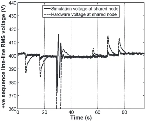
[image:7.594.39.286.69.268.2]The voltage tracking is shown in Figs. 12 and 13. In this case, a major deviation is visible during the DOL start when
Fig. 10. Scenario B: Frequency tracking between hardware and simulation.
Fig. 11. Scenario B: Phase tracking (angle by whichVNleadsV∗N).
[image:7.594.302.547.301.498.2] [image:7.594.301.550.533.740.2]Fig. 13. Scenario B: Voltage-tracking error.
the hardware voltage drops by more than 100 V (0.25 p.u.) for just over 2 s, while the simulation voltage oscillates around 400 V. During the DOL start, the active power reaches 35 kW, and reactive power reaches 45 kVAR, a total of 57 kVA, which is 71% of the rating of the 80 kVA generator. Smaller unwanted hardware voltage drops (and rises) of 10 V (0.025 p.u.) can be seen during the static load additions and removals (about 10 kVA each, which is 12% of the rating of the 80 kVA generator).
To achieve adequate tracking, the recommendation for the present system is therefore to limit sudden load steps in the hardware to less than 8 kVA, i.e., less than 10% of the rating of the generator. This should ensure peak transient phase-tracking errors within 5◦ and peak transient voltage-tracking errors within about 10 V (2.5%).
VI. CONCLUSION
The methods that have been presented in this paper allow entire power networks to be embedded as HIL. An effective new phase advance method for coping with the interface delay present in a PHIL environment has been presented, in which a measured/calibrated parametertC, equal to the interface delay time, is used to calculate a phase advance angle. This angle advance is then applied to the PHIL hardware generator control as an offset. This method avoids the requirement for unwanted artificial components to be added to the simulation, which is the traditional method to cope with interface delay.
In addition, in order to cope with the real-world prob-lems of antialias filter design and ADC skew, methods for accurately calibrating the measured amplitudes and phases of hardware voltages and currents have been developed and presented. These methods use a combination of time-domain and frequency-domain techniques which lead to reduced com-putational burden.
Using a synchronous generator as the interface between hard-ware and simulation has the constraint that neither harmonics nor unbalance can be deliberately injected into the hardware. There are also limits to the ROCOF and rate of change of voltage in simulation which can be tracked accurately. Using the described setup, tracking with peak errors of 5◦ (phase) and 1% (amplitude) can be achieved for simulation slew rates
of 0.25 Hz/s and 30 V/s for fast transient events. Hardware transients of up to 10% of the synchronous generator rating can also be accommodated with 5◦ (phase) and 2.5% (am-plitude) tracking errors. However, the use of a synchronous generator may allow brief hard faults to be placed in the hardware, with resulting currents much larger than 1 p.u. In contrast, an inverter would have to be significantly overde-signed with corresponding expense to allow such large currents to be accommodated without requiring a trip of the inverter itself.
To achieve the demonstrated phase-tracking accuracy, using a synchronous generator, a fast-responding prime mover in conjunction with a feedforward throttle control term has been used to good effect. The active power controls are almost as tight as can be achieved without the risk of instability, although early experiments into the use of a nonlinear slope in place of the linear gainKϕ show that this might yield some further reduction in phase-tracking error.
There are several opportunities for further work. It might be possible to improve the demonstrated voltage-tracking per-formance using some relatively inexpensive modifications. The addition of a feedforward term to the excitation control (feed-ing forward VAR flow to the field control) might provide some improvement. Furthermore, a more powerful solid-state excitation system for the synchronous generator would allow faster forcing of the field current to hit target voltage values, particularly during times of dynamically changing VAR flows. Only a single-channel device capable of±30 V and 20 A would be enough to excite the generator with the present slew rates, although a larger (bidirectional) voltage range would increase the field current slew rate and an oversized current rating would be a prudent measure. A lower leakage reactance of the generator would also be desirable, although this is an inherent property of the generator and cannot be reduced for the existing installation. The measurement averaging times of 112–5 cycles could also be reduced for the specific PHIL application, leading to improved tracking of both phase and amplitude. Finally, the simulation architecture and antialiasing filter design could be modified to reduce the magnitude of the 425 μs interface delay(tC).
REFERENCES
[1] A. Bouscayrol, X. Guillaud, P. Delarue, and B. Lemaire-Semail, “Ener-getic macroscopic representation and inversion-based control illustrated on a wind energy conversion systems using hardware-in-the-loop sim-ulation,”IEEE Trans. Ind. Electron., vol. 56, no. 12, pp. 4826–4835, Dec. 2009.
[2] B. Lu, X. Wu, H. Figueroa, and A. Monti, “A low-cost real-time hardware-in-the-loop testing approach of power electronics controls,”IEEE Trans. Ind. Electron., vol. 54, no. 2, pp. 919–931, Apr. 2007.
[3] D. Hercog, B. Gergic, S. Uran, and K. Jezernik, “A DSP-based remote control laboratory,”IEEE Trans. Ind. Electron., vol. 54, no. 6, pp. 3057– 3068, Dec. 2007.
[4] D. Zhang and H. Li, “A stochastic-based FPGA controller for an induction motor drive with integrated neural network algorithms,”IEEE Trans. Ind. Electron., vol. 55, no. 2, pp. 551–561, Feb. 2008.
[5] G. G. Parma and V. Dinavahi, “Real-time digital hardware simulation of power electronics and drives,”IEEE Trans. Power Del., vol. 22, no. 2, pp. 1235–1246, Apr. 2007.
[7] L. W. Qian, D. A. Cartes, and H. Li, “An improved adaptive detection method for power quality improvement,”IEEE Trans. Ind. Appl., vol. 44, no. 2, pp. 525–533, Mar./Apr. 2008.
[8] J. T. Bialasiewicz, “Renewable energy systems with photovoltaic power generators: Operation and modeling,”IEEE Trans. Ind. Electron., vol. 55, no. 7, pp. 2752–2758, Jul. 2008.
[9] S. K. Kim, J. H. Jeon, C. H. Cho, J. B. Ahn, and S. H. Kwon, “Dynamic modeling and control of a grid-connected hybrid generation system with versatile power transfer,”IEEE Trans. Ind. Electron., vol. 55, no. 4, pp. 1677–1688, Apr. 2008.
[10] Y. K. Lo, T. P. Lee, and K. H. Wu, “Grid-connected photovoltaic system with power factor correction,”IEEE Trans. Ind. Electron., vol. 55, no. 5, pp. 2224–2227, May 2008.
[11] N. Femia, G. Lisi, G. Petrone, G. Spagnuolo, and M. Vitelli, “Distributed maximum power point tracking of photovoltaic arrays: Novel approach and system analysis,”IEEE Trans. Ind. Electron., vol. 55, no. 7, pp. 2610– 2621, Jul. 2008.
[12] RTDS Technologies Inc., RTDS Hardware Overview. [Online]. Available: http://www.rtds.com/hardware.htm
[13] R. Kuffel, R. P. Wierckx, H. Duchen, M. Lagerkvist, X. Wang, P. Forsyth, and P. Holmberg, “Expanding an analogue HVDC simulator’s modelling capability using a real-time digital simulator (RTDS),” inProc. ICDS Digital Power Syst. Simul., 1995, p. 199.
[14] S. C. Verma, H. Odani, S. Ogawa, K. Kuroda, and Y. Kono, “Real time interface for interconnecting fully digital and analog simulators using short line or transformer,” inProc. IEEE Power Eng. Soc. Gen. Meet., 2006, 7 pp.
[15] X. Wu, S. Lentijo, and A. Monti, “A novel interface for power-hardware-in-the-loop simulation,” in Proc. IEEE Workshop Comput. Power Electron., 2004, pp. 178–182.
[16] S. Ayasun, R. Fischl, T. Chmielewski, S. Vallieu, K. Miu, and C. Nwankpa, “Evaluation of the static performance of a simulation-stimulation interface for power hardware in the loop,” inProc. IEEE Bologna Power Tech Conf., 2003, 8 pp.
[17] W. Ren, M. Steurer, and T. L. Baldwin, “Improve the stability and the ac-curacy of power hardware-in-the-loop simulation by selecting appropriate interface algorithms,”IEEE Trans. Ind. Appl., vol. 44, no. 4, pp. 1286– 1294, Jul./Aug. 2008.
[18] S. Woodruff, H. Boenig, F. Bogdan, T. Fikse, L. Petersen, M. Sloderbeck, G. Snitchler, and M. Steurer, “Testing a 5 MW high-temperature super-conducting propulsion motor,” inProc. Elect. Ship Technol. Symp., 2005, pp. 206–213.
[19] H. Li, M. Steurer, K. L. Shi, S. Woodruff, and D. Zhang, “Development of a unified design, test, and research platform for wind energy systems based on hardware-in-the-loop real-time simulation,”IEEE Trans. Ind. Electron., vol. 53, no. 4, pp. 1144–1151, Jun. 2006.
[20] Y. Liu, M. Steurer, and P. Ribeiro, “A novel approach to power quality assessment: Real time hardware-in-the-loop test bed,”IEEE Trans. Power Del., vol. 20, no. 2, pp. 1200–1201, Apr. 2005.
[21] J. Langston, S. Suryanarayanan, M. Steurer, M. Andrus, S. Woodruff, and P. F. Ribeiro, “Experiences with the simulation of a notional all-electric ship integrated power system on a large-scale high-speed electromagnetic transient simulator,” inProc. IEEE Power Eng. Soc. Gen. Meet., 2006, 5 pp.
[22] M. Armstrong, D. J. Atkinson, A. G. Jack, and S. Turner, “Power system emulation using a real time, 145 kW, virtual power system,” inProc. Eur. Conf. Power Electron. Appl., 2005, 10 pp.
[23] RTDS Technologies Inc., RSCAD Simulation Software. [Online]. Available: http://www.rtds.com/software.htm
[24] Applied Dynamics International, Real Time Station (RTS). [Online]. Available: http://www.adi.com/products_sim_tar_rts.htm
[25] A. J. Roscoe, “Systems and methods for performing analysis of a multi-tone signal,” U.S. Patent 2 005 075 812, Apr. 7, 2005.
[26] A. J. Roscoe, “Measurement, control and protection of microgrids at low frame rates supporting security of supply,” Ph.D. dissertation, Dept. Electron. Elect. Eng., Univ. Strathclyde, Glasgow, U.K., 2009.
[27] A. J. Roscoe, G. M. Burt, and J. R. McDonald, “Frequency and fundamen-tal signal measurement algorithms for distributed control and protection applications,”Proc. IET—Gener., Transm. Distrib., vol. 3, no. 5, pp. 485– 495, May 2009.
Andrew J. Roscoereceived the B.A. degree in elec-trical and information sciences tripos from Pembroke College, Cambridge, U.K., in 1991 and the M.Sc. degree in energy systems and the environment and the Ph.D. degree from the University of Strathclyde, Glasgow, U.K., in 2004 and 2009, respectively.
He was with GEC Marconi from 1991 to 1995, where he was involved in antenna design and cali-bration, specializing in millimeter-wave systems and solid-state phased array radars. From 1995 to 2004, he was with Hewlett Packard and, subsequently, Agilent Technologies, in the field of microwave communication systems, spe-cializing in the design of test and measurement systems for personal mobile and satellite communications. He is currently a Research Fellow with the Institute for Energy and Environment, Department of Electronic and Electrical Engi-neering, University of Strathclyde, working in the field of distributed generation and active network management. His recent projects include real-time pricing studies, the creation and deployment of microgrid control algorithms at the 100 kVA scale, the design/build of a 10 kVA three-phase inverter, new algo-rithms for the measurement of dynamic system parameters using low sample rates, and loss-of-mains detection strategies.
Andrew Mackayreceived the B.Eng. (Hons.) and M.Sc. degrees in electrical and electronic engineer-ing from the University of Strathclyde, Glasgow, U.K., in 2001 and 2003, respectively.
He is currently with Rolls-Royce PLC, Derby, U.K. He has worked on several projects involving real-time hardware-in-the-loop simulations, dc pro-tection on unmanned aerial vehicle platforms, loss of mains of distributed generation, and simulation of more electric aeronautic and marine systems.
Graeme M. Burt(M’95) received the B.Eng. de-gree in electrical and electronic engineering and the Ph.D. degree following research into fault-diagnostic techniques for power networks from the University of Strathclyde, Glasgow, U.K., in 1988 and 1992, respectively.
He currently holds a chair in Power Systems with the Institute for Energy and Environment, Depart-ment of Electronic and Electrical Engineering, Uni-versity of Strathclyde, where he is the Director of The Rolls-Royce University Technology Centre in Electrical Power Systems sponsored by Rolls-Royce. His current research interests lie in the areas of protection and control for distributed generation, power-system modeling and simulation, and active distribution networks.
J. R. McDonald (M’90) received the B.Sc. and Ph.D. degrees in electrical and electronic engineer-ing from the University of Strathclyde, Strathclyde, U.K., in 1978 and 1990, respectively.