The generalized identification of truly interfacial molecules (ITIM) algorithm for nonplanar interfaces

Identifying interfacial molecules in nonplanar interfaces: the

generalized ITIM algorithm

Marcello Sega∗

Tor Vergata University of Rome, via della Ricerca scientifica 1, I-00133 Rome, Italy

Sofia S. Kantorovich

Sapienza University of Rome, p.le A. Moro 4, I-00188 Rome, Italy and

Ural Federal University, Lenin Ave. 51, 620083 Ekaterinburg, Russia

P´al Jedlovszky

Laboratory of Interfaces and Nanosize Systems,

Institute of Chemistry, E¨otv¨os Lor´and University,

P´azm´any stny 1/a, H-1117 Budapest, Hungary

MTA-BME Research Group of Technical Analytical

Chemistry. Szt. Gell´ert t´er 4, H-1111 Budapest, Hungary and

EKF Department of Chemistry, H-3300 Eger, Le´anyka u. 6, Hungary

Miguel Jorge

LSRE/LCM-Laboratory of Separation and Reaction Engineering,

Faculdade de Engenharia, Universidade do Porto,

Rua Dr. Roberto Frias, 4200-465 Porto, Portugal

Abstract

We present a generalized version of theitimalgorithm for the identification of interfacial molecules,

which is able to treat arbitrarily shaped interfaces. The algorithm exploits the similarities between

the concept of probe sphere used in itim and the circumsphere criterion used in the α-shapes

approach, and can be regarded either as a reference-frame independent version of the former, or

as an extended version of the latter that includes the atomic excluded volume. The new algorithm

is applied to compute the intrinsic orientational order parameters of water around a DPC and a

cholic acid micelle in aqueous environment, and to the identification of solvent-reachable sites in

four model structures for soot. The additional algorithm introduced for the calculation of intrinsic

density profiles in arbitrary geometries proved to be extremely useful also for planar interfaces, as

I. INTRODUCTION

Capillary waves represent a conceptual problem for the interpretation of the properties of liquid-liquid or liquid-vapor planar interfaces, because long-wave fluctuations are smearing the density profile across the interface and all other quantities associated to it. This is usually overcome by calculating the density profile using a local, instantaneous reference frame located at the interface, commonly referred to as the intrinsic density profile, ρ(z) =

hA−1P

iδ(z−zi +ξ(xi, yi))i, where (xi,yi,zi) is the position of thei-th atom or molecule,

and the local elevation of the surface is ξ(xi, yi), assuming the macroscopic surface normal

being aligned with the Z axis of a simulation box with cross section area A. During the last decade several numerical methods have been proposed to compute the intrinsic density profiles at interfaces1–6. Despite several differences in these approaches, they are, in general, providing consistent distributions of interfacial atoms or molecules6 _{and density profiles}7_.

Among these methods, _itim4 _{proved to be an excellent compromise between computational}

cost and accuracy6, but it is limited to macroscopically flat interfaces, therefore there is a need to generalize it to arbitrary interfacial shapes.

Before these works, albeit for other purposes, several surface-recognition algorithms have been devised, and will be briefly mentioned below. All of them are possible starting points for the sought generalization under the condition that, once applied to the special case of a planar interface, they lead to consistent results with existing algorithms for the determination of intrinsic profiles.

Historically, the first class of algorithms addressing the problem of identifying surfaces was developed to determine molecular areas and volumes. The study of solvation proper-ties of molecules and macromolecules (usually, proteins) might require the identification of molecular pockets, or the calculation of the solvent-accessible surface area for implicit solva-tion models8_{. Two intuitive concepts are commonly used to describe the surface properties}

of molecules, namely, that of solvent-accessible surface9,10 _{(SAS), and that of molecular}

using a simple geometrical criterion. Many approximated13–24 _{or analytical}11,12,25–30

meth-ods have been developed to compute the MS or the SAS. In general, these methmeth-ods are based on discretization or tessellation procedures, requiring therefore the determination of the geometrical structure of the molecule. Other methods which allow to identify molecular surfaces include the approaches of Willard and Chandler5 _{or the Circular Variance method}

of Mezei31_{. Incidentally, the way the MS is computed in the early work of Greer and Bush}15

resembles very closely the itimalgorithm4.

From the late 1970s, the problem of shape identification had started being addressed by a newly born discipline, computational geometry. In this different framework, several algorithms have been actively pursued to provide a workable definition of surface, and in particular the concept of α-shapes32,33 _{showed direct implications for the determination of}

the molecular surfaces34,35. The approach based onα-shapes is particularly appealing due to its generality and ability to describe, besides the geometry, also the intermolecular topology of the system.

Noticeably, none of these methods – to the best of our knowledge – has ever been em-ployed for the determination of intrinsic properties at liquid-liquid or liquid-gas interfaces. Prompted by the apparent similarities between the usage of the circumsphere in the alpha shapes and that of the probe sphere in the itim method, as we will describe in the next

section, we investigated in more detail the connection between these two algorithms. As a result, we developed a generalized version ofitim(gitim) based on the α-shapes algorithm.

The new gitim method consistently reproduces the results of itim in the planar case while

retaining the ability to describe arbitrarily shaped surfaces. In the following we describe briefly the alpha shapes and the itimalgorithms, explain in detail the generalization of the

latter to arbitrarily shaped surfaces, and present several applications.

II. ALPHA SHAPES AND THE GENERALIZED ITIM ALGORITHM

The concept of α-shapes was introduced several decades ago by Edelsbrunner32,33_{. To}

date the method is applied in computer graphics application for digital shape sampling and processing, in pattern recognition algorithms and in structural molecular biology36_{. The}

compu-tational geometry37,38_{, which can be defined in several equivalent ways, for example, as the}

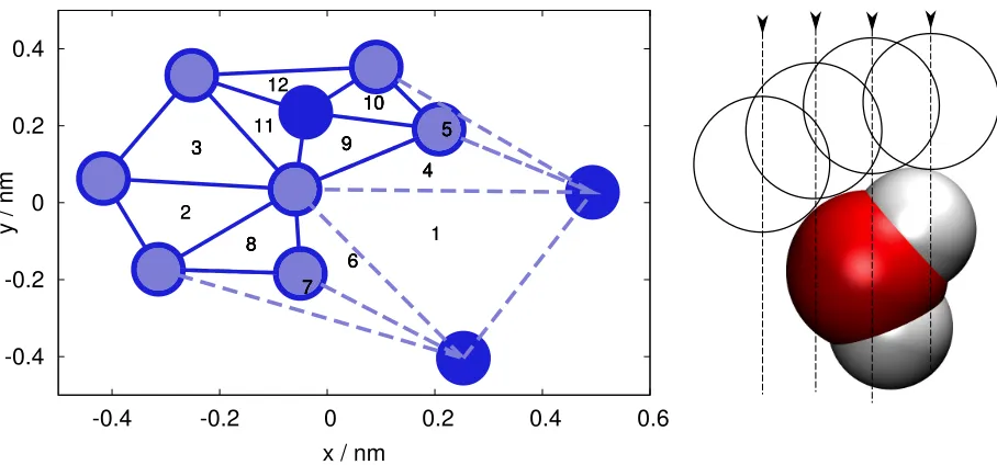
triangulation that maximizes the smallest angle of all triangles, or the triangulation of the centers of neighboring Voronoi cells. The idea behind the α-shapes algorithm is to perform a Delaunay triangulation of a set of points, and then generate the so-calledα-complex from the union of all k-simplices (segments, triangles and tetrahedra, for the simplex dimension k=1,2 and 3, respectively), characterized by a k-circumsphere radius (which is the length of the segment, the radius of the circumcircle and the radius of the circumsphere for k=1,2 and 3, respectively) smaller than a given value, α (hence the name). The α-shape is then defined as the border of theα-complex, and is a polytope which can be, in general, concave, topologically disconnected, and composed of patches of triangles, strings of edges and even sets of isolated points. In a pictorial way, one can imagine theα-shape procedure as growing probe spheres at every point in space until they touch the nearest four atoms. These spheres will have, in general, different radii. Those atoms that are touched by spheres with radii larger than the predefined value α are considered to be at the surface.

An example of the result of the α-shapes algorithm in two dimensions is sketched in Fig. 1a. The itim algorithm is based instead on the idea of selecting those atoms of one

phase that can be reached by a probe sphere with fixed radius streaming from the other phase along a straight line, perpendicular to the macroscopic surface. An atom is considered to be reached by the probe sphere if the two can come at a distance equal to the sum of the probe sphere and Lennard-Jones radii, and no other atom was touched before along the trajectory of the probe sphere. In practice, one selects a finite number of streamlines, and if the space between them is considerably smaller than the typical Lennard-Jones radius

Rp, the result of the algorithm is practically independent of the location and density of the

streamlines. The same is not true regarding the orientation of the streamlines; this is a direct consequence of the algorithm being designed for planar surfaces only. The basic idea behind the itimalgorithm are sketched in Fig. 1b. A closer inspection reveals that the condition of

being a surface atom for the_itim algorithm resembles very much that of theα-shapes case. Quadruplets of surface atoms identified by the itim algorithm have the characteristic of

sharing a common touching sphere having the same radius as the probe sphere. In this way, one can see the analogy with the α-shapes algorithm, the Rp parameter being used instead

ofα. The most important differences in theα-shapes algorithm with respect toitimare the

frame. We devised, therefore, a variant of the α-shapes algorithm that takes into account the excluded volume of the atoms.

In the approach presented here the usual Delaunay triangulation is performed, but the

α-complex is computed substituting the concept of the circumsphere radius with that of the radius of the touching sphere, thus introducing the excluded volume in the calculation of the α-complex. Note that this is different from other approaches that are trying to mimic the presence of excluded volume at a more fundamental level, like the weighted α-shapes algorithm, which uses the so-called regular triangulation instead of the Delaunay one33_{. In}

addition, in order to eliminate all those complexes, such as strings of segments or isolated points, which are rightful elements of the shape, but do not allow a satisfactory definition of a surface, the search for elements of the α-complex stops in our algorithm at the level of tetrahedra, and triangles and segments are not checked. In this sense gitim can provide

substantially different results from the original α-shapes algorithm.

The equivalent of the α-complex is then realized by selecting the tetrahedra from the Delaunay triangulation whose touching sphere is smaller than a probe sphere of radius Rp,

and the equivalent of the α-shape is just its border, as in the original α-shapes algorithm. The procedure to compute the touching sphere radius is described in the Appendix.

In the implementation presented here, in order to compute efficiently the Delaunay tri-angulation, we have made use of the quickhull algorithm, which takes advantage of the fact that a Delaunay triangulation in d dimensions can be obtained from the ridges of the lower convex hull in d+ 1 dimensions of the same set of points lifted to a paraboloid in the ancillary dimension39. The quickhull algorithm employed here40 has the particularly advan-tageous scalingO(Nlog(ν)) of its computing time with the numberN andν of input points and output vertices, respectively.

A separate issue is represented by the calculation of the intrinsic profiles (whether profiles of mass density or of any other quantity) as the distance of an atom in the phase of interest from the surface is not calculated as straightforwardly as in the respective non-intrinsic versions. For each atom in the phase, in fact, three atoms among the interfacial ones have to be identified in order to determine by triangulation7 _{the instantaneous, local position}

of the distances using O(NlogN) algorithms like quicksort, in favor of a better performing approach, based on kd-trees41,42_{, a generalization of the one-dimensional binary tree, which}

are still built in aO(NlogN) time, but allow for range search in (typically) O(logN) time.

III. COMPARISON BETWEEN THE ITIM AND THE GITIM METHODS

We have compared the results of the _itim and _gitim algorithms applied to the wa-ter/carbon tetrachloride interface composed of 6626 water and 966 CCl4 molecules. The

water and CCl4 molecules have been described by the TIP4P model43, and by the potential

of McDonald and coworkers44, respectively. The molecules have been kept rigid using the SHAKE algorithm45_{. This simulation, as well as the others reported in this work have been}

performed using the Gromacs46 _{simulation package employing an integration time step of}

1 fs, periodic boundary conditions, a cutoff at 0.8 nm for Lennard-Jones interactions and the smooth Particle Mesh Ewald algorithm47 _{for computing the electrostatic interaction,}

with a mesh spacing of 0.12 nm (also with a cut-off at 0.8 nm for the real-space part of the interaction). All simulations were performed in the canonical ensemble at a temperature of 300K using the Nos´e–Hoover thermostat48,49 _{with a relaxation time of 0.1 ps. A simulation}

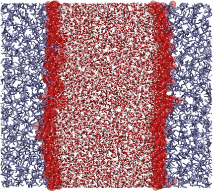
snapshot of the H2O/CCl4 interface is presented in Fig. 2, where the surface atoms

identi-fied by the gitim algorithm using a probe sphere radius of 0.25 nm are highlighted using a

spherical halo.

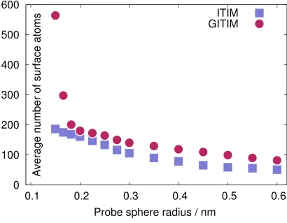
We have used the itim and gitim algorithms to identify the interfacial atoms of the

water phase in the system, for different sizes of the probe sphere. In general,gitimidentifies

systematically a larger number of interfacial atoms thanitimfor the same value of the probe

sphere radius Rp, as it is clearly seen in Fig. 3. Remarkably, for values of the probe sphere

radius smaller than about 0.2 nm (compare, for example, with the optimal _itimparameter

Rp = 0.125 nm suggested in Ref. 6), the interfacial atoms identified bygitim show the onset

of percolation. The reason for this behavior traces back to the fact that itim is unable to

identify voids buried in the middle of the phase, as it is effectively probing only the cross section of the voids along the direction of the streamlines. This difference could explain the higher number of surface atoms identified by gitim, as voids in a region with high local

spheres can be thought as inflating at every point in space instead of moving down the streamlines, and this is the reason why the algorithm is able to identify also small pockets inside the opposite phase.

It is possible to make a rough but enlightening analytical estimate of the probability for a probe sphere of null radius in the itimalgorithm to penetrate for a distanceζ in a fluid of

hard spheres with diameterσ and number densityρ. Using the very crude approximation of randomly distributed spheres, the probabilityp0 to pass the first molecular layer, at a depth ζ = σ is the effective cross section p0 = 1− π₄ρ2/3σ2, and that of reaching a generic depth ζ can be approximated as p(ζ) = pζ/σ₀ , where κ = ln(1/p0)/σ defines a penetration depth. Therefore, using a probe sphere with a null radius, itim will identify a (diffuse) surface at

a depth 1/κ, while _gitim will identify every atom as a surface one. For water at ambient conditions, the penetration is κ−1 ' 0.186 nm, a distance smaller than the size of a water molecule itself. This could explain why in Ref. 6, even using a probe sphere radius as small as 0.05 nm, almost only water molecules in the first layer were identified as interfacial ones by

itim (see the almost perfectly Gaussian distribution of interfacial water molecules in Fig.9

of Ref. 6).

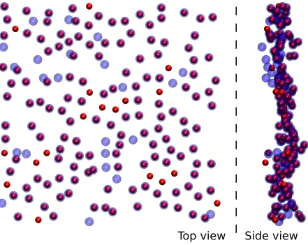
Nevertheless, it is important for practical reasons to be able to match the outcome of both algorithms. It turns out that choosing Rp so that the average number of interfacial

atoms identified by both algorithms is roughly the same leads also, not surprisingly, to very similar distributions. The probe sphere radius required forgitim to obtain a similar average

number of surface atom as initimcan be obtained by an interpolation of the values reported

in Fig. 3. An example showing explicitly the interfacial atoms identified by the two methods (Rp = 0.2 nm for itim and Rp = 0.25 nm for gitim) is presented in Fig. 4: roughly 85%

of surface atoms are identified simultaneously by both methods, demonstrating the good agreement between the two methods once the probe sphere radius has been re-gauged. The condition of identifying the same atoms as interfacial ones is much more strict that any condition on average quantities, like the spatial distribution of interfacial atoms or intrinsic density profiles. Hence, it is expected that a good agreement on such quantities can also be achieved.

The intrinsic density profiles of water and carbon tetrachloride are reported in Fig. 5, as computed byitimand gitim, respectively, with the interfacial water molecules as reference.

the same as described in Ref. 7. Starting from the projection P0 = (x, y) of the position of

the given atom to the macroscopic interface plane, the two interfacial atoms closest to P0

are found (their position on the interface plane being P1 and P2, respectively). The third

closest atom with projection P3 has then to be found, with the condition that the triangle

P1P2P3 contains the point P0. A linear interpolation of the elevation of P0 from those of

the other points is eventually performed, and employed to compute the distance z−ξ(x, y) which is used to compute the intrinsic density profile.

Efficient neighbor search for the P1, P2 and candidate P3 atoms is implemented using

kd-trees42 as discussed before. The two pairs of profiles are very similar, besides a small difference in the position and height of the main peak of the CCl4 profile (curves on the

right in Fig. 5) and in the minimum of the water profile (curves on the left in Fig. 5) right next to the surface position, which are anyway compatible with the differences observed between various methods for the calculation of intrinsic density profiles7_{. The delta-like contribution}

of the water molecules at the surface is included in the plot in Fig. 5, and defines the origin of the reference system. Negative values of the signed distance from the interface correspond to the aqueous phase.

IV. THE PROBLEM OF NORMALIZATION OF DENSITY PROFILES

Before applying_gitimto non-planar interfaces, one important issue has still to be solved, namely that of the proper calculation of intrinsic density profiles in non-planar geometries. In general, one uses one-dimensional density profiles (intrinsic or non-intrinsic) when the system is, or is assumed to be, invariant under displacements along the interface, so that the orthogonal degrees of freedom can be integrated out. When the interface has a non-planar shape, one needs to use a different coordinate system. In the case of a quasi-spherical object for example, one could use the spherical coordinate system to compute the non-intrinsic density profile, and normalize each bin by the integral of the Jacobian determinant, that is the volume of the shell at constant distance from the origin. In the intrinsic case, however, it is necessary to know at every time step the volume of the shells at constant distance from the interface.

storage overhead. Here, instead, we propose to employ an approach based on simple Monte Carlo integration: in parallel with the calculation of the histograms for the various phases, we compute also that of a random distribution of points, equal in number to the total atoms in the simulation. The volume of a shell can be estimated as box volume times the ratio of the number of points found at a given distance and the total number of random points drawn. We are following the heuristic idea that for each framej one does not need to know the volume of the shell Vj(r) with a precision higher than that of the average number of

atoms in it, Nj(r). In addition, we assume that the surface area of the interface is large

enough for the shell volume variations δVj(r) to be small with respect to its average value

ˆ

V(r) = PN

j Vj(r)/N. The average density

ρ(r) = 1

N

N

X

j=1 Nj(r)

Vj(r)

(1)

can be approximated as

ρ(r)' 1 N

1 ˆ

V(r)

N

X

j=1

"

Nj(r)−Nj(r)

δVj(r)

ˆ

V(r) #

. (2)

When the relative volume changes|δV /V|are small, one can therefore simply normalize the histogram ˆN(r) =PN

j Nj(r)/N by the average volume ˆV(r) obtained by the Monte Carlo

procedure, disregarding the terms of order O(δV /Vˆ).

The correctness of our assumption is demonstrated incidentally by the application of this normalization once again to the planar case. The thin lines in Fig. 5 represent the

itimintrinsic mass density profile of water and carbon tetrachloride, using the Monte Carlo

for macroscopically planar interfaces. The calculation of the Monte Carlo normalization factors does not change the typical scaling of the algorithm, as it consists in calculating the histogram for an additional phase of randomly distributed points (which effectively behaves as an ideal gas). The better accuracy at larger distances, however, demonstrates that the use of the Monte Carlo normalization is much more efficient than the standard approach, as it requires much smaller systems to be able to extract the same information (e.g., to resolve the fourth peak in Fig. 5, an additional slab of about 2-3 nm would have been needed). In this sense, the Monte Carlo normalization procedure can be even beneficial in terms of performance.

V. EXAMPLES OF NON-PLANAR INTERFACES

A. DPC micelle

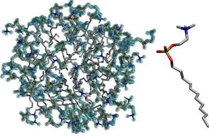
Dodecylphosphocholine (DPC) is a neutral, amphiphilic molecule with a single fatty tail that can form micelles in solution: these play a relevant role in biochemistry, especially for NMR spectroscopy investigations aiming at understanding the structure of proteins or peptides bound to an environment that is similar to the biological membrane50–53. The molecular structure of DPC is shown in Fig.6. We have simulated for 500 ps a micelle of 65 DPC and 6305 water molecules using the force field and configurations from Tieleman and colleagues54, and have calculated the intrinsic mass density profiles of both phases (DPC and water) usinggitim and the Monte Carlo normalization procedure, with a probe sphere

radius Rp = 0.25. The result of the interfacial atoms identification on the DPC micelle for

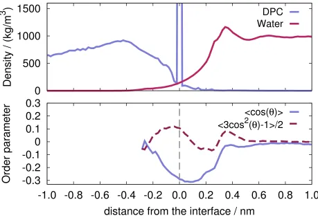
a single frame is shown in Fig. 6, where water molecules have been removed for the sake of clarity, and interfacial atoms are highlighted as usual with a halo. The intrinsic mass density profile, calculated relative to the DPC surface, is reported in Fig. 7, with the DPC mass density profile shown on the left, and the water profile on the right.

As usual, the delta-like contribution at r = 0 identifies the contribution from interfacial DPC atoms. In addition, we have calculated, for the first time, the intrinsic profiles of the orientational order parameters S1 and S2 of the water molecules around the DPC micelle.

The two parameters are defined asS1 =hcos(θ1)iandS2 =h3 cos2(θ2)−1i/2, whereθ1 and

center), and the water molecule symmetry axis and molecular plane normal, respectively. The orientation is taken so that θ1 < π/2 when the hydrogen atoms are farther from the

micelle than the corresponding oxygen. The complete picture of the orientation of water molecules would be delivered by the calculation of the probability distribution p(θ1, θ2)55,56, but here we limit our analysis to the two separate order parameters and their intrinsic profiles. Note that, since these quantities are computed per particle, there is no need to apply any volume normalization. The polarization of water molecules, which is proportional toS1, appears to be different from zero only very close to the micellar surface. In particular, S1 has a correlation with the main peak of the intrinsic density profile in the proximity of 0.4 nm. Water molecules located closer to the interface show a first change in the sign of the polarization and a subsequent one when crossing the interface. Farther than 0.25 nm inside the micelle, not enough water molecules are found to generate any meaningful statistics. Also the S2 order parameter is practically zero beyond 0.6 nm, and again a correlation is seen

with the main peak of the intrinsic density profile, and the maximum in the orientational preference is found just next to the interface, where S1 ' 0, showing that water molecules

are preferentially laying parallel to the interfacial surface.

B. Soot

One of the main byproducts of hydrocarbon flames, soot is thought to have a relevant impact on atmospheric chemistry and global surface warming58,59. Electron, UV, and atomic force microscopy have revealed the size and structure of soot particles from different sources at different scales60–64. In particular, soot emitted by aircraft is found to be made of several, quasi-spherical, concentric graphitic layers of size in the range from 5 to 50 nm60_{. We have}

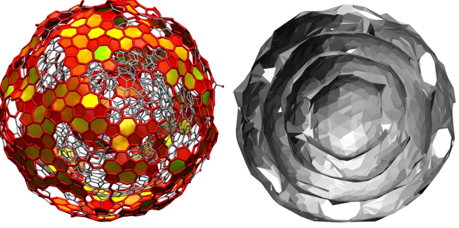
used four model structures (SI

1,SI2, SI4 and SII from Ref. 57) to demonstrate the ability of gitimto identify surface atoms in complex geometries. In Fig. 8, the SI1model is represented

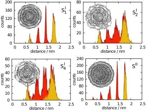
in section as a triangulated surface (right), showing the four concentric layers, and in whole (left) showing the surface atoms as detected by _gitim using Rp = 0.25 nm. The histograms

This finding is in a clear accordance with the results of the void analysis and adsorption isotherm calculations presented in Ref. 57.

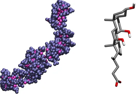
C. Secondary cholic acid micelle

Bile acids, such as cholic acid are biological amphiphiles built up by a steroid skeleton and side groups attached to it. The organization of these side groups is such that hydrophilic and hydrophobic groups are located at the two opposite sides of the steroid ring. Thus, bile acids have a hydrophilic and a hydrophobic face (often referred to as the α and β side, respectively) rather than a polar head and an apolar tail, as in the case of other surfactants like, for example, DPC. The unusual molecular shape leads to peculiar aggregation behavior of bile acids. At relatively low concentrations they form regular micelles with an aggregation number of 2-10, while above a second critical micellar concentration these primary micelles form larger secondary aggregates by establishing hydrogen bonds between the hydrophilic surface groups of the primary micelles65,66_{. These secondary micelles are of rather irregular}

shape,66,67 _{which makes them an excellent test system for our purposes.}

Here we analyze the surface of a secondary cholic acid micelle composed of 35 molecules, extracted from a previous simulation work66 and simulated for the present purposes for 500 ps in aqueous environment. An instantaneous snapshot of the micelle is shown in Fig.10 (water molecules are omitted for clarity) together with a schematic structure of the cholic acid molecule. We calculated the density profile of water as well as of cholic acid relative to the intrinsic surface of the micelle by the gitim method. The resulting profiles are shown

VI. CONCLUSIONS

In this paper we presented a new algorithm that combines the advantageous features of both theitimmethod4and theα-shapes algorithm32,33to be used in determining the intrinsic

surface in molecular simulations. Thus, unlike the original variant, this new, generalized version of _itim, dubbed _gitim, is able to treat interfaces of arbitrary shapes and, at the same time, to take into account the excluded volumes of the atoms in the system. It should be emphasized that the gitim algorithm is not only able to find the external surface of the

phase of interest, but it also detects the surface of possible internal voids inside the phase. The method, based on inflating probe spheres up to a certain radius in points inside the phase turned out to provide practically identical results with the originalitim analysis for planar

interfaces. Further, its applicability to non-planar interfaces was shown for three previously simulated systems, i.e., a quasi-spherical micelle of DPC54_{, molecular models of soot}57_{, and}

a secondary micellar aggregate of irregular shape built up by cholic acid molecules66_.

Another important result of this paper concerns the correct way of calculating density profiles relative to intrinsic interfaces, irrespective of whether they are macroscopically planar or not. Thus, here we proposed a Monte Carlo-based integration algorithm to estimate the volume elements in which points of the profile are calculated, in order to normalize them correctly. The issue of normalization with the volume elements in macroscopically flat fluid interfaces originates from the fact that these interfaces are rough on the molecular scale, namely, at the length scale of the calculated profiles. We clearly demonstrated that using this new normalization the artificial smearing of the intrinsic density profiles far from the intrinsic interface can be avoided.

Two computer programs that implement, respectively, an optimized version of itim and

the newgitimalgorithm, as well as the calculation of intrinsic density and order parameters

Acknowledgements

M.S. acknowledges FP7-IDEAS-ERC grant DROEMU: “Droplets & Emulsions: Dynamics & Rheology” for financial support, and Gy¨orgy Hantal for providing the soot structures. Part of this work has been done by M.S. at ICP, Stuttgart University. P.J. is grateful for financial support from the Hungarian OTKA foundation under Project Nr. 104234. S.K. is supported by FP7-IDEAS-ERC Grant PATCHYCOLLOIDS and RFBR Grant mol a 12-02-31374. Simulation snapshots were made with VMD68_.

VII. APPENDIX

Here, following Ref. 69 we derive the expressions for the radiusRand positionr= (x, y, z) of the center of the sphere which is touching four other ones, having given radii and center positions Ri and ri = (xi, yi, zi) (i = 1,2,3 or 4), respectively. The conditions of touching

can be expressed with the following nonlinear system of four equations:

|r−ri|2 = (R+Ri)2. (3)

By subtracting one of them from the other three (without loss of generality we subtract the one with i = 1), the quadratic term, r2, will be eliminated and the system Eq.(3) would become linear with respect to r:

Mr =s−Rd, (4)

where the matrix M and the vectors d and s are defined as

M=     

r1−r2

r1−r3

r1−r4



   

, d= 

   

R1−R2 R1−R3 R1−R4

     , (5) and

s= 1 2      

r2₁−r2₂−R₁2+R2₂

r2

1−r23−R12+R23

r2

1−r24−R12+R24

      . (6)

either does not exist, or is not unique):

r=M−1s−RM−1d ≡r0−Ru, (7)

whereM−1_s=r

0 andu=M−1d. Once Eq.(7) is substituted into the first of the constraints

Eq.(3), it leads to the quadratic algebraic equation with respect toR:

1− |u|2

R2+ 2 (R1−u·v)R+ (R21− |v|2) = 0, (8)

where v=r1−r0. The solution of Eq. (8) can be found in the following form:

R± =

−(R1−u·v)± |R1u+v|

1− |u|2 . (9)

If|u|2 _{is not equal to unity (which corresponds to the case when the 4 spheres are tangential}

to one plane), then Eq.(9) provides two different solutions, and the positive one provides the radius R of the touching sphere as a function of the centre position r. Eventually, the positions of their centres can be obtained by inserting R into Eq.(7). In the present manuscript in case of two possible solutions we choose the sphere with minimal radius.

∗ _{Electronic address: [email protected]}

1 _{E. Chac´on and P. Tarazona, Phys. Rev. Lett.91, 166103 (2003).}

2 _{J. Chowdhary and B. M. Ladanyi, J. Phys. Chem. B110, 15442 (2006).}

3 _{M. Jorge and M. N. D. S. Cordeiro, J. Phys. Chem. C 111, 17612 (2007).}

4 _{L. B. P´artay, G. Hantal, P. Jedlovszky, A. Vincze, and G. Horvai, J. Comput. Chem. 29,}

945 (2008).

5 _{A. P. Willard and D. Chandler, J. Phys. Chem. B 114, 1954 (2010).}

6 _{M. Jorge, P. Jedlovszky, and M. N. D. S. Cordeiro, J. Phys. Chem. C 114, 11169 (2010).}

7 _{M. Jorge, G. Hantal, P. Jedlovszky, and M. N. D. S. Cordeiro, J. Phys. Chem. C 114, 18656}

(2010).

8 _{J. Tomasi, B. Mennucci, and R. Cammi, Chem. Rev. 105, 2999 (2005).}

9 _{B. Lee and F. M. Richards, J. Mol. Biol. 55, 379 (1971).}

10 _{F. M. Richards, Annu. Rev. Biophys. Bioeng. 6, 151 (1977).}

12 _{M. L. Connolly, Science 221, 709 (1983).}

13 _{A. Shrake and J. Rupley, J. Mol. Biol. 79, 351371 (1973).}

14 _{F. Richards, J. Mol. Biol. 8, 2114 (1974).}

15 _{J. Greer and B. L. Bush, Proc. Natl. Acad. Sci. USA 75, 303 (1978).}

16 _{T. Richmond and F. Richards, J. Mol. Biol. 119, 537555 (1978).}

17 _{C. Alden and S.-H. Kim, J. Mol. Biol. 132, 411434 (1979).}

18 _{S. Wodak and J. Janin, Proc. Natl. Acad. Sci. USA77, 17361740 (1980).}

19 _{J. Muller, J. Appl. Cryst. 16, 7482 (1983).}

20 _{M. Pavlov and B. Fedorov, Biopolymers 22, 15071522 (1983).}

21 _{J. Pascual-Ahuir and E. Silla, J. Comput. Chem. 11, 10471060 (1990).}

22 _{H. Wang and C. Levinthal, J. Comput. Chem. 12, 868871 (1991).}

23 _{S. Grand and K. J. Merz, J. Comput. Chem. 14, 349352 (1993).}

24 _{J. Weiser, P. S. Shenkin, and W. C. Still, J. Comp. Chem. 20, 217 (1999).}

25 _{M. Connolly, J. Am. Chem. Soc.107, 11181124 (1985).}

26 _{T. Richmond, J. Mol. Biol. 178, 6389 (1984).}

27 _{K. Gibson and H. Scheraga, Mol. Phys. 62, 12471265 (1987).}

28 _{K. Gibson and H. Scheraga, Mol. Phys. 64, 641644 (1988).}

29 _{C. Kundrot, J. Ponder, and F. Richards, J. Comp. Chem. 12, 402409 (1991).}

30 _{G. Perrot, B. Cheng, K. Gilson, K. Palmer, A. Nayeem, B. Maigret, and et al., J. Comp.}

Chem. 13, 111 (1992).

31 _{M. Mezei, J. Mol. Graphics. and Modell. 21, 463 (2003).}

32 _{H. Edelsbrunner, D. Kirkpatrick, and R. Seidel, IEEE Trans. on Information Theory 29, 551}

(1983).

33 _{H. Edelsbrunner and E. M¨ucke, ACM T. Graphic.13, 43 (1994).}

34 _{H. Edelsbrunner, M. Facello, P. Fu, and J. Liang, Measuring proteins and voids in proteins,}

in Proc. 28th Annu. Hawaii Intl. Conf. System Sciences, volume 5, p. 256264, Los Alamitos,

California, 1995, IEEE Computer Society Press.

35 _{J. Liang, H. Edelsbrunner, P. Fu, P. V. Sudhakar, and S. Subramanian, Proteins 33, 1}

(1998).

36 _{H. Edelsbrunner, Handbook of Discrete and Computational Geometry, edited by J. E. Goodman}

37 _{B. N. Delaunay, Izv. Akad. Nauk SSSR, Otdelenie Matematicheskii i Estestvennyka Nauk 7,}

793800 (1934).

38 _{A. Okabe, B. Boots, K. Sugihara, and S. N. Chiu, Spatial Tessellations: Concepts and}

Applications of Voronoi Diagrams, Wiley, Chichester, U.K., 2000.

39 _{D. Brown, Inf. Process. Lett. 9, 223228 (1979).}

40 _{C. Barber, D. Dobkin, and H. Huhdanpaa, ACM T. Math. Software 22, 469 (1996).}

41 _{J. L. Bentley, Cmmun. ACM 18, 509 (1975).}

42 _{J. Bentley and J. Friedman, ACM Compu. Sur. 11, 397 (1979).}

43 _{W. L. Jorgensen, J. Chandrashekar, J. D. Madura, R. Impey, and M. L. J. Klein, Chem.}

Phys. 79, 926 (1983).

44 _{I. R. McDonald, D. G. Bounds, and M. L. Klein, Mol. Phys. 45, 521 (1982).}

45 _{J. P. Ryckaert, G. Ciccotti, and H. J. C. Berendsen, J. Comput. Phys. 23, 327 (1977).}

46 _{B. Hess, C. Kutzner, D. van der Spoel, and E. Lindahl, J. Chem. Theory Comput. 4, 435}

(2008).

47 _{U. Essmann, L. Perera, M. Berkowitz, T. Darden, H. Lee, and L. Pedersen, J. Chem. Phys.}

103, 8577 (1995).

48 _{S. Nos´e, Mol. Phys. 52, 255 (1984).}

49 _{W. Hoover, Phys. Rev. A 31, 1695 (1985).}

50 _{A. Rozek, C. Friedrich, and R. Hancock, Biochemistry 39, 15765 (2000).}

51 _{J. Gesell, M. Zasloff, and S. Opella, J. Biomol. NMR 9, 127 (1997).}

52 _{D. Schibli, R. Montelaro, and H. Vogel, Biochemistry 40, 9570 (2001).}

53 _{D. Kallick, M. Tessmer, C. Watts, and C. Li, J. Magn. Reson. Ser. B 109, 60 (1995).}

54 _{D. Tieleman, D. Van der Spoel, and H. Berendsen, J. Phys. Chem. B 104, 6380 (2000).}

55 _{P. Jedlovszky, ´A. Vincze, and G. Horvai, J. Chem. Phys. 117, 2271 (2002).}

56 _{P. Jedlovszky, ´A. Vincze, and G. Horvai, Phys. Chem. Chem. Phys. 6, 1874 (2004).}

57 _{G. Hantal, S. Picaud, P. Hoang, V. Voloshin, N. Medvedev, and P. Jedlovszky, J. Chem.}

Phys. 133, 144702 (2010).

58 _{J. Quaas, Nature 471, 456 (2011).}

59 _{S. van Renssen, Nature Clim. Change 2, 143 (2012).}

60 _{O. Popovitcheva, N. Persiantseva, M. Trukhin, G. Rulev, N. Shonija, Y. Buriko, A. Starik,}

61 _{L. Sgro, G. Basile, A. Barone, A. D’Anna, P. Minutolo, A. Borghese, and A. D’Alessio,}

Chemosphere51, 1079 (2003).

62 _{Y. Chen, N. Shah, A. Braun, F. Huggins, and G. Huffman, Energ. Fuel 19, 1644 (2005).}

63 _{A. Abid, N. Heinz, E. Tolmachoff, D. Phares, C. Campbell, and H. Wang, Combust. Flame}

154, 775 (2008).

64 _{A. Abid, E. Tolmachoff, D. Phares, H. Wang, Y. Liu, and A. Laskin, P. Combust. Inst 32,}

681 (2009).

65 _{D. Small, Chemistry; The Bile Acids, edited by P. P. Nair, D. Kritchevsky, volume 1, chapter 8,}

Plenum Press, New York, 1971.

66 _{L. P´artay, P. Jedlovszky, and M. Sega, J. Phys. Chem. B111, 9886 (2007).}

67 _{L. P´artay, M. Sega, and P. Jedlovszky, Langmuir23, 12322 (2007).}

68 _{W. Humphrey, A. Dalke, and K. Schulten, J. Molec. Graphics 14, 33 (1996).}

-0.4 -0.2 0 0.2 0.4

-0.4 -0.2 0 0.2 0.4 0.6

y / nm

x / nm

1 1 2 2 3 3 3 3 4 4 4 4 5 5 5 5 6 6 6 7 7 7 7 8 8 8 8 9 9 9 9 10 10 10 10 11 11 12 12

FIG. 1: Left: example of theα-shapes algorithm on a set of points on the plane. The lines connecting

the atoms represent the Delaunay triangulation (the triangles are labeled by numbers from 1 to

12). Solid lines mark triangles belonging to the α-complex, and dashed lines those which are not.

The light-shaded atoms are those belonging to the α-shape, the border of the α-complex. Two

atoms (in triangle 1) are outside the α-shape, and one (shared by triangles 9-12) is inside the

α-shape. Right: schematic representation of theitimalgorithm, applied to a single water molecule:

FIG. 2: Simulation snapshot of a H2O/CCl4system. The oxygen atoms at the interface between the

H2O phase (inner) and CCl4 phase (outer) as recognized by the gitim algorithm are represented

with an additional halo. Unconnected points belong to molecules which cross periodic boundary

0

100

200

300

400

500

600

0.1

0.2

0.3

0.4

0.5

0.6

Average number of surface atoms

Probe sphere radius / nm

ITIM

GITIM

FIG. 3: Average number of surface atoms identified by itim (squares) and gitim (circles) as a

FIG. 4: Water surface oxygen atoms in the H2O/CCl4 system in one simulation snapshot as

rec-ognized by gitimexclusively (small spheres), itimexclusively (large spheres) or by both methods

0

500

1000

1500

2000

2500

3000

3500

-2

-1.5

-1

-0.5

0

0.5

1

1.5

2

Density / (kg / m

3

)

Position relative to the interface / nm

ITIM (H

O)

GITIM (H

O)

ITIM (CCl

)

GITIM (CCl

)

ITIM+MC (CCl

)

ITIM+MC (H

O)

FIG. 5: Intrinsic density profiles of water (curves on the left) and carbon tetrachloride (curves on

the right) with respect to the water surface as computed with itim (solid curves) or with gitim

(dashed curves). The thin curves are computed using itim and the Monte Carlo normalization

FIG. 6: Right: schematic structure of a DPC molecule. Left: snapshot of a DPC micelle in water.

Only the DPC constituents are shown for the sake of clarity. Atoms with a halo are those recognized

0

500

1000

1500

Density / (kg/m

3

)

DPC

Water

-0.3

-0.2

-0.1

0

0.1

0.2

0.3

-1.0 -0.8 -0.6 -0.4 -0.2 0.0

0.2

0.4

0.6

0.8

1.0

Order parameter

distance from the interface / nm

<cos(

θ

_)>

<3cos

(

θ

_)-1>/2

FIG. 7: Upper panel: intrinsic density profiles of water (right) and of DPC (left). Lower panel:

intrinsic profile of the orientational order parameters (P1, solid line, P2, dashed line). The vertical

FIG. 8: The SI

1 soot model57 represented in section (right, triangulated surface) and in whole

(left, wireframe) with the atoms identified bygitim as surface ones highlighted using thicker, red

elements. Besides surface atoms, also chemical bonds between surface atoms are highlighted, as

FIG. 9: Histograms of the atoms in the four soot models taken from Ref. 57. Each panel refers to

a different structure (depicted with wireframe), and presents the distribution of all atoms (filled,

darker area) and of surface atoms identified by gitim (filled, lighter area), as a function of the

FIG. 10: Left: simulation snapshot of a secondary cholate micelle, with surface atoms highlighted.

0

500

1000

1500

2000

2500

-0.4

-0.2

0

0.2

0.4

0.6

0.8

1

Density / ( kg / m

3

)

Position relative to the interface / nm

Cholate

Water