Optimal geometric motion planning for a spin-stabilized spacecraft

Optimal geometric motion planning for spin-stabilized

spacecraft

James D. Biggs

Nadjim Horri

A method requiring low-computational overhead is presented which generates low-torque reference

mo-tions between arbitrary orientamo-tions for spin-stabilized spacecraft. The initial stage solves a constrained

opti-mal control problem deriving analytical solutions for a class of smooth and feasible reference motions.

Specif-ically, for a quadratic cost function an application of Pontryagin’s maximum principle leads to a completely

integrable Hamiltonian system that is, exactly solvable in closed-form, expressed in terms of several free

pa-rameters. This is shown to reduce the complexity of a practical motion planning problem from a constrained

functional optimization problem to an unconstrained parameter optimization problem. The generated

refer-ence motions are then tracked using an augmented quaternion feedback law, consisting of the sum of a

propor-tional plus derivative term and a term to compensate nonlinear dynamics. The method is illustrated with an

application to re-point a spin-stabilized agile micro-spacecraft using zero propellant. The low computational

overhead of the method enhances its suitability for on-board motion generation.

Keywords: nonholonomic motion planning, parametric optimization, Pontryagin’s maximum principle, attitude

control, tracking .

I.

Introduction

Spin stabilization and three-axis stabilization are methods used to maintain the pointing direction of spacecraft.

With spin stabilization the entire spacecraft rotates around its own pointing axis using the gyroscopic effect.1

Ad-∗_{[email protected], Advanced Space Concepts Laboratory, Department of Mechanical & Aerospace Engineering, University of}

Strath-clyde, Glasgow, G1 1XJ, UK.

†_{[email protected], Surrey Space Centre, Faculty of Engineering and Physical Sciences, University of Surrey, Guildford, Surrey, GU2 7XH,}

vantages of spin stabilization are that it is a simple and passive way of keeping the spacecraft pointing in a certain

direction. Designers of early satellites used spin-stabilization and examples include NASA’s Pioneer 10 and 11

space-craft, the Lunar Prospector, and the Galileo Jupiter orbiter. The dynamics and control of spin stabilized spacespace-craft,

under varying mission assumptions, have been extensively researched, see for example.2–5 _{Such passive control is}

particularly attractive to limited resource spacecraft which can switch off their active GNC system during passive

stabilization and use the battery power to perform operational tasks. However, a disadvantage of passive stabilization

is that it cannot be used to accurately re-point the antennas or optical instruments. Therefore, missions that require

frequent re-pointing tend to use three-axis stabilization. Three-axis stabilization can be achieved with gas jet actuators

or reaction wheels using classical attitude control methods such as proportional plus derivative (PD) type controllers,

based on quaternion-feedback for large angle maneuvers6or eigenaxis rotations.7

The development of nano and micro-spacecraft (from the 1 kg Cubesat to the more enhanced micro-spacecraft of

around 150 kg) are cost effective alternatives to conventional spacecraft that pose new engineering challenges. One

such challenge is that their small reaction wheels can generate a very limited torque for active control. For example

Surrey Satellite Technology Limited (SSTL) is now developing a reaction wheel with a maximum torque capability

of 0.1 Nm, for future use on micro-satellites (100kg-150kg). Therefore, in order to design propellant free maneuvers

for micro-spacecraft the reference motions have to be trackable within 0.1 Nm. Once the desired pointing direction

has been obtained the spacecraft should use passive control to save battery power. Therefore, for micro spacecraft

it is desirable to use spin stabilization to maintain a pointing direction and perform small-torque motions (feasible

with reaction wheels) for re-pointing. This type of maneuver could be achieved by “de-spinning” the pointing axis,

performing a conventional rest-to-rest eigenaxis rotation and finally “spinning-up” around the pointing axis for passive

stabilization. However, this three stage manoeuver is a highly inefficient procedure and in general would not be feasible

with small torque.

This paper proposes a method requiring low-computational power for generating low-torque reference motions

for spacecraft constrained to spin about a single axis. By closely tracking this reference motion the spacecraft will

minimize the “spin-up” or “de-spin” of the pointing axis providing gyroscopic stiffness and using small accumulated

torque. The design of such low-torque reference motions subject to constraints are often formulated and solved in

the context of constrained optimal control problems. These type of problems generally define the attitude kinematics

subject to prescribed boundary conditions and inequality constraints such as bounding the instantaneous torque.8–19

In particular, designing minimum accumulated torque motions using pseudo-spectral direct transcription methods has

proved instrumental in saving the International Space Station large amounts of precious propellant.20This method can

however be computationally demanding. Other optimization approaches such as the locally optimal Euler Lagrange

approach of calculus of variations were used to solve problems such as time-optimal attitude control21and the

mini-mum fuel problem for a fixed time horizon.22These local methods have the added complexity of numerically solving

two point boundary value problems onboard the satellite. The Hamilton-Jacobi-Bellman (HJB) approach from

dy-namic programming is globally stabilizing, but is numerically intractable. Solving it off-line is possible numerically,23

but the global optimal solution is only approximated up to a certain order, which cannot be too high for practical

im-plementation. For attitude control applications, these numerical optimization techniques are therefore still traditionally

avoided onboard small micro-satellites with limited computational resources, such as those developed by SSTL.

The method in this paper uses geometric control theory24–26_{to reduce the computational expense of the}

optimiza-tion procedure. Geometric control theory has been used to derive coordinate free necessary and sufficient condioptimiza-tions

for attitude controllability using gas jet actuators and momentum exchange devices. Furthermore, these results were

used to design coordinate free control laws that stabilize the system around an equilibrium state.27 Given the

control-lability of the system it is then desirable to plan a feasible and if possible optimal motion to track. Motion planning

for systems defined on Lie groups, e.g. in this case the Special Orthogonal Group SO(3), has been tackled using

parameterizations of the manifold and using averaging to design small re-orientations.28 However, this method is

inadequate to perform large slew maneuvers and a global approach is required. A coordinate free formulation of an

optimal control problem was proposed for the attitude motion planning of a spacecraft in Spindler.29 For a trivial

case of constant optimal angular velocities exact solutions for the corresponding rotations were derived. However,

for time-dependent optimal angular velocities the method in29reverts to using numerical shooting methods, requiring

numerical integration, in order to match the prescribed final orientation. Furthermore, this motion planning problem

did not take torque requirement into consideration when planning motions.

In this paper, a method is proposed that can rapidly generate low-torque reference motions with low-computational

overhead enabled through the machinery of geometric mechanics and control. Although the application of geometric

control theory to solve left-invariant optimal control problems and their reduction to quadratures on 3-D Lie groups is

that,for a spacecraft constrained to spin about one axis, the necessary conditions for optimality are guaranteed exactly

with respect to a quadratic cost function. The analytic form of the solution then enables the construction of a practical

cost function analytically which, in turn, requires the optimization of only a few free parameters. Specifically,

Pon-tryagin’s maximum principle enables the original motion planning problem to be reformulated as an unconstrained

parameter optimization problem, thus, greatly reducing the computational demand. Moreover, a numerical

optimiza-tion of a few parameters is used to match a prescribed final orientaoptimiza-tion while minimizing torque during the manoeuver.

An augmented quaternion feedback is then used to track the designed reference motions.

This paper is presented as follows: In Section II, the kinematic and dynamic models used are introduced. Although

the equations for the rigid body are well known they are included here as the kinematics are expressed as quaternions

and equivalently in the less conventional matrix form on the Special Unitary GroupSU(2). The quaternion

differen-tial equations are better suited for numerical integration as they do not have singularities and are conventionally used

on-board spacecraft. Furthermore, the compact kinematic formulation onSU(2)is also used as they enable the most

natural and elegant analytical treatment in the derivation of the optimal motions. In Section III, the derivation of a

general form for the optimal motions in terms of several free parameters is given via Pontryagin’s maximum principle

and Lax pair integration.24–26The method assigns a simple quadratic cost function to the kinematic equations that

con-strain the rotational motion of the spinning axis about the pointing direction. It is then shown that the optimal angular

velocity inputs are simple sinusoidal functions. This result viewed independently does not explicitly offer any new

in-sight into the control problem as sinusoidal control of nonholonomic systems has already been covered extensively.30

However, as the sinusoidal velocity inputs are derived in the setting of geometric mechanics and control it allows the

corresponding motion to be derived completely analytically using Lax Pair integration.24, 25 The derived closed-form

analytic expressions then enable the rapid generation of feasible reference motions. In Section IV, an unconstrained

numerical parameter optimization method is undertaken to optimize the available parameters of the analytic solution

to match the prescribed end-points and minimize accumulated torque amongst this subset of admissible motions.

In Section V, a method is proposed to track the generated reference motions and a proof of the closed-loop stability

is given in the appendix. Finally, an example is given which shows the reference motions to be feasible by the tracking

controller, which is applied to perform re-pointing manoeuvres for a spin-stabilized agile earth observation SSTL

II.

Models

The equations describing the attitude control problem are that of an asymmetric rigid body with external forces

describing the effect of the reaction wheel torques. These consist of kinematic equations relating the angular position

to the angular velocity, and the dynamic equations describing the evolution of angular velocity or, equivalently, angular

momentum.

A. Kinematic equations

To obtain a global description of the problem the angular position is usually denoted by a rotation matrix in the

Special Orthogonal GroupSO(3). In addition the angular position maybe described locally by parameterizing the

rotation matrix using Euler angles.27However, in this paper both a quaternion representation and an equivalent matrix

formulation on the Special Unitary GroupSU(2)is used (SU(2)is isomorphic to the unit quaternions25). Again this

representation is used as the quaternion differential equations are conventionally used on board spacecraft and are

suited to numerical integration as they do not possess singularities. In addition the formulation onSU(2)is used as it

is the most natural and convenient for the analytical calculations. In terms of the angular velocityΩ1,Ω2,Ω3in the

body frame the quaternion representation of kinematics are taken to be:

dq¯

dt =

1 2 ˆ

Ωq¯ (1)

where ¯q= [q0,q]T = [q0,q1,q2,q3]T withq0,q1,q2,q3∈Ror equivalently expressed as ¯q=q0e+q1i+q2j+q3k

is the unit quaternion whereeis a four-dimensional unit vector and where its orthogonal complimenti,j,kform a

right-handed orthonormal frame,q= [q1,q2,q3]T is known as the vector part of the quaternion and fully determines

the attitude where:

ˆ

Ω=



           

0 −Ω1 −Ω2 −Ω3

Ω1 0 Ω3 −Ω2

Ω2 −Ω3 0 Ω1

Ω3 Ω2 −Ω1 0



           

(2)

attitude propagation singularities. This representation is equivalent to the kinematic matrix representation onSU(2):

dR(t)

dt =R(t)(Ω1A1+Ω2A2+Ω3A3) (3)

whereR(t)∈SU(2)represents the spacecrafts orientation,A1,A2,A3form a basis for the Lie algebrasu(2)of the Lie

groupSU(2):

A1=

1 2     i 0

0 −i



  

,A2=

1 2     0 1 −1 0    

,A3=

1 2     0 i i 0     (4)

whereiis an imaginary number and the Lie algebra’s commutator defined by[X,Y] =Y X−XY called the Lie bracket

withX,Y∈su(2)such that[A1,A2] =−A3,[A2,A3] =−A1and[A1,A3] =A2whereR(t)∈SU(2)is of the form:

R(t) =



  

z1 z2

−¯z2 z¯1



  

(5)

withz1,z2∈Cand ¯z1,z¯2their complex conjugates such that|z1|2+|z2|2=1. Physically the basisA1,A2,A3describe

the infinitesimal motion of the spacecraft in the roll, pitch and yaw directions respectively. Furthermore, the two sets

of kinematic equations (1) and (3) are equivalent with the isomorphismF:SU(2)↔H:

F:



  

z1 z2

−¯z2 z¯1



  

↔z1+z2·j=q0e+q1i+q2j+q3k (6)

defining the coordinate change and where the complex numbersz1=q0+iq1,z2=q2+iq3 are regarded in their

quaternion formz1=q0e+q1i,z2=q2e+q3isubject to the usual quaternionic multiplication. For more details of this

isomorphism see25pp. 169-171.

B. Dynamic equations

The Euler equations with external forces are used to represent the attitude dynamics of a spacecraft with reaction wheel

actuators:

IΩ˙ =−Ω×IΩ+u⇔

˙

Ω1=δ1Ω2Ω3+

u1

I1

˙

Ω2=δ2Ω1Ω3+

u2

I2

˙

Ω3=δ3Ω1Ω2+

u3

I3

(7)

whereδ1=I2−_I1I3, δ2=I3−_I2I1, δ3=I1−_I3I2 whereI1,I2,I3are the principal moments of inertia andIis the moment

axes of the satellite and is given byu=−˙h−Ω×hwhereΩ= [Ω1, Ω2, Ω3]T and the vectorhrepresents the

angular momentum of the wheels.

III.

Analytic derivation of the reference motion

The initial formulation of the motion planning problem is presented in the context of a constrained functional

optimization problem that includes equality constraints and a performance index (an integral function of the angular

velocities). This formulation ensures smooth and feasible motions are defined and enable the derivation of analytic

solutions in closed form. This renders a class of feasible curves subject to the equality constraint that satisfy the

neces-sary conditions for optimality. This analytic form essentially reduces the original constrained functional optimization

problem to an unconstrained parameter optimization problem where the parameters are chosen to match the

bound-ary conditions and minimize accumulated torque. The initial motion planning problem is defined by the kinematic

constraint (equality constraint):

dR(t)

dt =R(t)(vA1+Ω2A2+Ω3A3) (8)

where the roll axis in constrained to spin at a constant rate Ω1=v. Note that this also includes the possibility

of performing maneuvers where the pointing direction is constrained to have zero spin v=0. Amongst all

ad-missible motions of (8) we seek solutions that minimize the functional l(R(t)) =RT

0

D_dR(t)

dt , dR(t)

dt

E

dt between the

given boundary conditions R(0) =R0 andR(T) =RT whereT is a fixed-terminal time and h·,·i=−1₂trace(·,·)

is the trace form. As the trace form is left (respectively right) invariant this is equivalent to minimizingl(R(t)) =

RT

0

D

R(t)−1dR(t)

dt ,R(t)

−1dR(t)

dt

E

dtand from (8) it follows thatl(R(t)) = 1₂RT

0 v2+Ω22+Ω23dt. Asvis constant on the

fixed-time intervalT this is equivalent to minimizing the performance index:

f0=

1 2

Z T

0

Ω22+Ω23dt (9)

It is easily shown that this problem is controllable and therefore this optimal control problem is well posed.24, 25 This

initial cost function is not conventional but it is meaningful since (i) it ensures smooth motions (ii) it minimizes the

integral of angular velocities on the unconstrained axes which avoids the system accumulating more angular velocity

than needed (iii) it avoids dangerously fast slew rates while making sure that the final attitude is specified (not at rest

in final time but with small bounded final velocity) and (iv) using the machinery of geometric control theory it allows

Theorem 1 The class of reference motions that minimize the cost function (9) subject to the equality constraint (8)

are defined by :

Ω∗2=rsin((v+c)t+β), Ω∗3=rcos((v+c)t+β) (10)

q∗₀=(K−c)cos( 1

2t(c−K+v))+(K+c)cos(12t(c+K+v))

2K

q∗₁=(K−c)sin( 1

2t(c−K+v))+(K+c)sin(12t(c+K+v))

2K

q∗₂=±r

Ksin

_(v+c)

2 t+β

sin K₂t

q∗₃=±r

Kcos

_(v+c)

2 t+β

sin K₂t

(11)

whereΩ∗₁=v,Ω∗₂Ω∗₃are the optimal angular velocities and q₀∗,q∗₁,q∗₂,q∗₃the corresponding quaternion components

subject to the given boundary conditionsq¯∗(0) = [1 0 0 0]T andq¯∗(T) =q¯T and where r,c,β are parameters

available for optimization, v is the given spinning angular velocity and K=√c2_+r2_{is a constant.}

Proof

The Hamiltonian corresponding to the left-invariant kinematic constraint (8) that minimises the function (9) is:24–26

H(p,u) =vp(A1) +Ω2p(A2) +Ω3p(A3)−ρ0(

1 2(Ω

2

2+Ω23)) (12)

whereρ0>0 is a fixed positive constant and p(·):su(2)7→Rsuch that p(Ai)are scalar components of an element

in the dual of the Lie algebrasu(2)∗, withρ0=1 for regular extremals andρ0=0 for abnormal extremals. It can be

shown that the abnormal extremals are projections of the regular extremals so setρ0=1 (see Jurdjevic (1997)25 for

details). Following this define the linear functionsλi=p(Ai)fori=1,2,3 then from the Maximum Principle and the

fact that (12) is a concave function the optimal velocity inputs are given by _ddH_Ω

i =0 and thereforeΩ

∗

2=λ2,Ω

∗

3=λ3

Substituting these values into (12) gives the optimal Hamiltonian

H∗=vλ1+

1

2 λ

2 2+λ32

(13)

Defining the Poisson Bracket{λi,λj}=−p([Ai,Aj])where[Ai,Aj]is the Lie bracket then ˙λi={H,λi}is:

˙

λ1=0, λ˙2=λ3(v−λ1), λ˙3=−λ2(v−λ1) (14)

whereλ1,λ2,λ3∈su∗(2). For convenience we defineλ1=−cwherecis a constant. Defining a reduced constant

HamiltonianHr=2(H∗+cv)givesHr=λ22+λ32then parameterizingHr using polar coordinatesλ2=rsinθ,λ3=

rcosθ givesr=Hr1/2andθis given as follows:

θ=arctan

λ2

λ3

then

˙

θ=λ3

˙

λ2−λ2λ˙3

λ₂2+λ₃2 (16)

substituting ˙λ2and ˙λ3from (14) into (16) yields:

˙

θ=v+c (17)

thereforeθ=C1t+β whereC1=v+candβ is a constant of integration. To obtain the corresponding quaternions,

we use the Lax pair representation of the regular extremals:25

dL(t)

dt = [L(t),∆H] (18)

where

L(t) =λ1A1+λ2A2+λ3A3, ∆H=vA1+λ2A2+λ3A3 (19)

with general solution:

L(t) =R(t)−1L(0)R(t) (20)

equivalently

R(t)L(t)R(t)−1=L(0) (21)

whereL(0)is a matrix of constant entries andR(t)L(t)R(t)−1describes the conjugacy class ofL(t)and therefore an

initialR(0)can be chosen such thatL(0) =KA1. Therefore, it suffices to integrate the particular solution:

¯

R(t)L(t)R¯(t)−1=KA1 (22)

therefore

L(t) =KR¯(t)−1A1R¯(t) (23)

as exp(ϕ1A1)is the stabilizer ofA1it is convenient to introduce the coordinate form:

¯

R(t) =exp(ϕ1A1)exp(ϕ2A2)exp(ϕ3A1) (24)

and substituting into (23) yields:

L(t) =iK

2



  

cosϕ2 e−iϕ3sinϕ2

eiϕ3_sinϕ

2 −cosϕ2



  

(25)

then equating (25) withL(t)in (19) yields

which can also be simplified to obtain:

tanϕ3=

λ2

λ3

(27)

to obtain an expression forϕ1substitute (24) into (3) and simplify using the previously derived expressions to yield:

˙

ϕ1=K (28)

and define the initial angle to beϕ1(0) =γ which yieldsϕ1=Kt+γ. Substitutingϕ2andϕ3in from equations (26)

and (27) into (24) and pulling the solution back to the identity via:

R(t) =RintR¯(0)−1R¯(t) (29)

whereRintis the initial orientation and ¯R(0)−1is the inverse of ¯R(t)att=0 gives the solution onSU(2). Finally, using

the isomorphism (6) yields (11). Q.E.D.

This defines analytically a subset of admissible smooth motions expressed in terms of several free parameters. Note

that the sign ofq2,q3in (11) is dependent on choosing the frame to be positively or negatively oriented. For this

analytic solution to correspond with the numerical solution of the differential equation (1) this frame is taken to be

negatively oriented. The following section assigns analytically derived cost functions (also functions of the same free

parameters) which can be numerically optimized to minimize the accumulated torque and prescribed final orientation

error. This initial constrained optimal control problem defined amongst all admissible curves has been reduced to a

class of analytically defined feasible curves. This essentially reduces the motion planning problem to an unconstrained

parameter optimization problem.

IV.

Unconstrained parameter optimization

The previous section derives an analytic description of a class of smooth, feasible motions expressed as functions

of the parametersv,r,c,β(10,11). The problem now is to choose the free parametersr,c,βsuch that the boundary

con-ditions are matched at the terminal timet=T (they are not included in the original performance index) and such that

accumulated torque is minimized. In order to match a prescribed final pointing direction ¯qf = [qf0 qf1 qf2 qf3]T

at the terminal timet=T to high-precision the available parameters can be optimized to minimize the performance

index:

In addition, when planning a motion for micro-spacecraft it is essential to minimize torque during the manoeuver. A

cost functional that penalizes torque requirement can be expressed in terms of these free parameters. Substituting (10)

andΩ1=vinto (7) yields the control torque inputu= [u1, u2, u3]T:

u1=−(1/2)I1r2sin(2(t(c+v) +β))δ1

u2=I2rcos(t(c+v) +β) (c+v−vδ2)

u3=−I3rsin(t(c+v) +β) (c+v+vδ3)

(31)

Then to minimize the accumulated torque over the time interval t ∈[0,T] the available parameters r,c,β can be

optimized such that the functional:

J2=

T

Z

0

hu,ui2dt (32)

is minimized. This integral can be evaluated analytically and equates to finding the minimum of the analytic function:

J2=

r2

32α 

       

r2(4Tα+sin(4β))−sin(4(Tα+β))I₁2δ₁2

+8(2Tα−sin(2β) +sin(2(Tα+β))I₂2(α+vδ2)2

+8(2Tα+sin(2β)−sin(2(Tα+β))I₃2(α+vδ3)2



       

(33)

whereα=v+c. Therefore, to obtain the optimal parameters for the reference motion (10,11) the multi-objective

function:

J=J1+kJ2 (34)

is minimized, whereJ1andJ2are defined in (30) and (33) respectively and wherekis a weighting parameter. Given

the moments of inertiaI1,I2,I3, spinning angular velocityvand terminal timeT this problem is easily solved using

unconstrained numerical parameter optimization.

V.

Re-pointing an agile spin stabilized micro-spacecraft

In this section the methodology is applied to perform a large slew-manoeuver for a spin-stabilized spacecraft.

The model of an agile earth observation micro-satellite (based on a small satellite platform from Surrey Satellite

Technology Limited (SSTL)) is used for the numerical simulation study. The moments of inertia of the micro-satellite

are given byI1=19.5 kgm2,I2=19 kgm2,I3=12.6 kgm2. The less significant cross terms of the moment

of inertia matrix are neglected for simplicity. A feasible spinning velocity constraint ofv=0.2 rads−1is assumed.

200 secs (a reasonable time-scale for such a manoeuver to be performed with admissible torque). Two unconstrained

parameter optimizations of the performance index (34) were undertake for comparison using Mathematica:31(i) when

k=0 and (ii) when k=1/10. When k=0, the numerical parameter optimization returns the parameter values

r=0.6754,c=−3.6494×10−8_{,β=−56.1358. Substituting these values into (30) and (33) yieldsJ}

1=2.1982×10−7

andJ2=5.5684 respectively. By comparison, whenk=1/10 an unconstrained numerical optimization yields the

parametersr=0.0157,c=−7.1920×10−8,β =0.4204. Substituting these values into (30) and (33) yieldsJ1=

4.2081×10−6_andJ

2=0.0026. Comparing the two results it can be seen that there is an inevitable trade off between

final orientation error and accumulated torque depending on the weightk. However, there is only a small increase in

final orientation error when compared to the decrease in accumulated torque. Moreover, whenk=0 it was found that

the resulting reference motion could not be tracked effectively with micro-reaction wheels (maximum torque of 0.1

Nm). However, as is now shown the reference motion generated fork=1/10 is trackable using micro-reaction wheels.

Substituting the generated parameters r=0.0157,c=−7.1920×10−8_{,β =0.4204 into (10) yields the reference}

angular velocities:

Ω∗₁=0.2 rads−1

Ω∗₂=0.015708 sin(0.420394+0.2t) rads−1

Ω∗₃=0.015708 cos(0.420394+0.2t) rads−1

(35)

and substituting these parameters into (11) yields the corresponding reference quaternion components:

q∗₀=0.5 cos(0.092146t) +0.5 cos(0.107854t)

q∗₁=0.5 sin(0.092146t) +0.5 sin(0.107854t)

q∗₂=−sin(0.4204+0.1t)sin(0.00785398t)

q∗₃=−cos(0.4204+0.1t)sin(0.00785398t)

(36)

finally substituting the generated parameters into (31) gives the theoretical torque history required to track this

refer-ence motion:

u1=−0.000789567 sin(2(0.420359+0.2t))Nm

u2=0.0813672 cos(0.420359+0.2t)Nm

u3=−0.0411548 sin(0.420359+0.2t)Nm

(37)

Following a transient tracking stage which will depend on controller gains and initial conditions, the actual torque

equation (37). The tracking of this reference motion is performed by the augmented quaternion feedback controller:6

u=−h˙−Ω×h=−kpIqe−kdIΩe+Ω×IΩ+IΩ˙∗ (38)

wherekpandkdare scalar gains being multiplied by the moment of inertia matrixIto make sure that gains are higher

on the axes with a higher moment of inertia. The vectorsqeandΩedenote the vector part of the quaternion tracking

error and the angular velocity tracking error vector respectively.

Note that the variable uwas introduced to simplify the stability proof in the appendix. The first two terms of

the control law (38) are used to tune the convergence rate and to adjust the damping characteristic, which varies

nonlinearly. The third term is a gyroscopic coupling nonlinearity and the last term is added to compensate for the

acceleration errors that would otherwise result from the time variability of the optimal angular velocities. The proposed

tracking approach, based on PD quaternion feedback with compensation of nonlinearities, is chosen as it has been

flight proven for other control objectives with time varying trajectories such as Sun tracking. It is also adequate for the

tracking of smooth trajectories, guarantees stability and only requires the tuning of two gains.

In practice, the control input is the control torque vector of the wheels−˙h, which is easily obtained using the fact

that−_h˙_{=u+Ω×h. The wheels momentahi,i=1,3 can then be integrated from an initial value and the wheels}

speed commands are easily obtained by division about the wheels moments of inertiaIwhi. The quaternion error is

obtained using the quaternion composition rule. More explicitly, the angular velocity error and quaternion error are

respectively given by:

Ωe=Ω−Ω∗, q¯e=Q∗q¯ (39)

whereQ∗=



           

q∗₄ q∗₃ −q∗₂ −q∗₁

−q∗₃ q∗₄ q∗₁ −q∗₂

q∗₂ −q∗₁ q∗₄ −q∗₃

q∗₁ q∗₂ q∗₃ q∗₄



           

is defined from the quaternion command vector ¯q∗= [q∗₀,q₁∗,q∗₂,q∗₃]from

equation (36).

The differential equation for the angular velocity error can be trivially obtained from equation (39). The differential

equation for the quaternion error ¯qehas an analogous form to the one for the actual quaternion ¯q:

dq¯e

dt =

1

where ˆΩedenotes the matrix form of the angular velocity error of the form (2), ¯qe= [qe0,qTe]T = [qe0,qe1,qe2,qe3]T

and the equation (40) is similar to equation (1) by taking the components of ¯qerather than those of ¯q.

The stability proof is provided in the appendix. The controller tuning is performed experimentally through

exten-sive numerical simulation. In the literature, there is an algorithmic approach for tuning the gain in the special case of

small eigenaxis rotations satisfyingΩ=θ˙eandq=sin(θ/2)e. Under the assumption of rest-to-rest maneuvers, the

closed loop system reduces to a second order oscillator6which can be used to determine the gain. Although this paper

deals with global, large slew-motions the use of this procedure6was used to get a first estimate of the gains. In addition

the procedure of the trial and error simulations are made simpler here by making the gain matrices proportional to the

moment of inertia matrix, meaning that only two gains need to be determined, despite this being a three axis control

problem.

A torque saturation limit of 0.1 Nm is considered in this simulation study. A sampling time of 1 second is used,

that is, all measurements of attitude, angular velocity and control torque are available every second. Furthermore,

zero order holds of 1 second are included in the model which essentially keep the continuous variables constant for 1

second. Initial angular velocity and quaternion errors were introduced to illustrate that the controller does not require

a transient velocity control stage before activation.

After extensive numerical simulations of the resulting closed loop dynamics (in nonzero momentum mode), three

sets of controller parameters were chosen , in three separate simulations, to illustrate the effect of controller parameters

on tracking performance and torque expenditure:

Low tracking gains : kp=0.025, kd=0.16

Medium tracking gains : kp=0.06, kd=0.48

High tracking gains : kp=0.5, kd=4.5

(41)

Note that these gains were chosen to compare tracking performance for similar damping characteristics. Increasing

the derivative gains further on the axes with time varying desired velocities was found not to necessarily increase

damping on all axes because of the system’s nonlinearity.

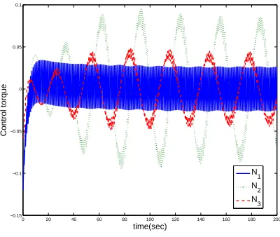
For a final boundary condition at 200 seconds, Figure 1 shows the control torque required to track the optimal

angular velocity trajectories with the high set of gainskp=0.5,kd=4.5, while Figure 2 shows the same plot for

low gainskp=0.025,kd=0.16. The simulation shows that the control torque is feasible using 0.1 Nm wheels with

0 20 40 60 80 100 120 140 160 180 200 −1

−0.8 −0.6 −0.4 −0.2 0 0.2

Time(sec)

Control torque (Nm)

N

1

N

2

N

3

Figure 1. Control torque of the reaction wheels- High gains

0 20 40 60 80 100 120 140 160 180 200 −0.15

−0.1 −0.05 0 0.05 0.1

time(sec)

Control torque

N

1

N

2

N

3

Figure 2.Control torque of the reaction wheels- Low gains

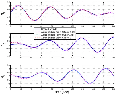
(37) are approached closely at steady state after transient errors. Figure 3 shows that the angular velocity tracking is

enhanced at steady state, but not at the transient time, by increasing the gains. Figure 4 shows that the attitude tracking

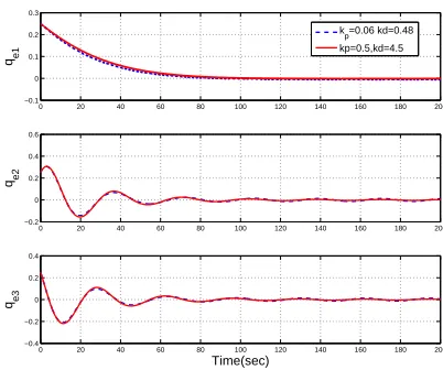
performance is enhanced on all three axes at steady states, but not at the transient time, by increasing the PD gains.

Figure 5 also shows a similar trend.

Note that although the results show that the torque requirement for good tracking is feasible for micro-spacecraft,

the required torque capability can be reduced by increasing the time horizon of the unconstrained numerical parameter

0 20 40 60 80 100 120 140 160 180 200 0.16 0.18 0.2 0.22 0.24 ω3 (rad/sec)

0 20 40 60 80 100 120 140 160 180 200 −0.06 −0.04 −0.02 0 0.02 ω2 (rad/sec)

0 20 40 60 80 100 120 140 160 180 200 −0.06 −0.04 −0.02 0 0.02 time(sec) ω3 (rad/sec) Desired velocity Actual velocity (kp=0.025,0.16) Actual velocity (kp=0.06,kd=0.48) Actual velocity (kp=0.5,kd=4.5)

Figure 3. Tracking of the desired angular velocity

0 20 40 60 80 100 120 140 160 180 200 −1.5 −1 −0.5 0 0.5 1 1.5 q1

0 20 40 60 80 100 120 140 160 180 200 −1.5 −1 −0.5 0 0.5 1 1.5 q2

0 20 40 60 80 100 120 140 160 180 200 −1.5 −1 −0.5 0 0.5 1 1.5 time(sec) q3 Desired attitude Actual attitude (kp=0.025,kd=0.16) Actual attitude (kp=0.06,kd=0.48) Actual attitude (kp=0.5,kd=4.5)

Figure 4. Tracking of the desired attitude

VI.

Conclusion

This paper has presented a method for generating low-torque attitude reference motions requiring low-computational

overhead for spin-stabilized spacecraft. It was further illustrated through simulation that these motions can be tracked

with admissible torque using reaction wheels onboard a micro-satellite. The procedure used for the motion planning

0 20 40 60 80 100 120 140 160 180 200 −0.1

0 0.1 0.2 0.3

qe1

0 20 40 60 80 100 120 140 160 180 200 −0.2

0 0.2 0.4 0.6

qe2

0 20 40 60 80 100 120 140 160 180 200 −0.4

−0.2 0 0.2 0.4

Time(sec)

qe3

k_p=0.06 kd=0.48 kp=0.5,kd=4.5

Figure 5. Quaternion errors

problem via Pontryagin’s maximum principle. A numerical parameter optimization was then employed to minimize

the final orientation error, between the actual and desired final orientation, and the accumulated torque during the

mo-tion. One of the main advantages of this approach is that it requires the optimization of only a few parameters and thus

is able to rapidly generate low-torque reference motions using low-computational power. It was further shown that

the reference motions can be tracked by limited resource spacecraft using an augmented version of the conventional,

flight tested, quaternion feedback law. In particular, it was illustrated that a generated large slew reference motion was

feasible for a near term micro-spacecraft with admissible torque and good tracking performance.

Appendix

The stability of the system with the controller of equation (38) can be shown with respect to the following Lyapunov

function:

V=kp(q2e1+q2e2+q2e3+ (1−qe4)2) +

1 2Ω

T

eΩe (42)

The first term can be simplified using the norm conservation property of the quaternion:

V=2kp(1−qe4) +

1 2Ω

T

eΩe (43)

The differentiation ofVleads to :

˙

By substitutinguby its expression from equation (38), we have:

˙

V =kpΩTeqe+ΩTeI

−1_(−k

pIqe−kdIΩe+IΩ˙∗−IΩ˙∗) (45)

A number of terms in the last equation cancel and the resulting time derivative ofVreduces to:

˙

V=−kdΩT_eΩe<0 ∀Ωe6=0 (46)

At the equilibrium point,V(q¯e= [1,0,0,0]T,Ωe= [0,0,0]T) =0, we haveV =0. Convergence to the equilibrium

follows from Lasalle’s invariance principle.33

PD feedback with compensation of nonlinearities is known to be robust in practice to the bounded disturbances that

are linearly related to attitude dynamics and nearly periodic functions of time. For applications requiring robustness

under arbitrary bounded disturbance torques, an alternative would be to substitute the PD terms by a sliding mode term

or to simply add a sliding mode term to robustify the stabilizing controller, as proposed by Luo et al.32

References

1_{Sidi, M. J., ‘Spacecraft Dynamics and Control: A practical engineering approach ’, Cambridge University Press, 2002.}

2_{Hall C, D., Rand. R, H., ‘Spinup Dynamics of Axial Dual-Spin Spacecraft’, Journal of Guidance, Control and Dynamics, Vol. 17, No. 1, pp.}

30:37, 1994

3_{Meehan, P. A., Asokanthan, S. F., ‘Control of Chaotic Motion in a Dual-Spin Spacecraft with Nutational Damping’, Journal of Guidance,}

Control and Dynamics, Vol. 25, No. 2, pp. 209:214, 2002.

4_{Bao, G. W., Pascal, M., ‘Stability of a Spinning Liquid-filled Spacecraft, Applied Mechanics, Vol. 67, pp. 407:421, 1997.}

5_{Tsiotras, P., Longuski, J. M., ‘Spin-axis Stabilization of Symmetric Spacecraft with Two Control Torques’, Systems and Control Letters, Vol.}

23, pp. 395:402, 1994.

6_{Wie, B., Barba, P. M. ‘Quaternion feedback for spacecraft large-angle maneuvers’. Journal of Guidance, Control and Dynamics, vol. 8, No.}

3, pp. 360-365, 1985.

7_{Wie, B., Weiss, H.,Arapostathis, A. ‘Quaternion feedback regulator for spacecraft eigenaxis rotations’. Journal of Guidance, 12, 375380,}

1989.

8_{Scrivener, S. L., Thompson, R. C. ‘Survey of Time-Optimal attitude Maneuvers’. Journal of Guidance, Control, and Dynamics, Vol. 17, No.}

2, pp. 225-231, 1994.

9_{Vadali, S.R., Junkins, J.L. ‘Optimal open loop and stable feedback control of rigid spacecraft attitude maneuvers’, Journal of Astronautical}

10_{Junkins,J. L., Carrington, C. K., and Williams, C. E., ‘Time-optimal magnetic attitude maneuvers,’ J. Guidance, Control, and Dynamics, vol.}

4, no. 4, pp. 363368, 1981.

11_{Byers, R. M., and Vadali, S. R. ‘Quasi closed-form solution to the time-optimal rigid spacecraft reorientation problem,’ AAS Paper 91120,}

1991.

12_{Etter, J. R., ‘A solution of the time-optimal Euler rotation problem,’ AIAA Paper 89-3601-CP, 1989.}

13_{Tsiotras, P., ‘Stabilization and Optimality Results for the Attitude Control Problem’ Journal of Guidance Control and Dynamics Vol.19, No.}

4, July-August 1996.

14_{Athans, M. , Falb, P. L., and Lacoss, R. T., ‘Time-, fuel-, and energy optimal control of nonlinear norm-invariant systems,’ IRE Trans.}

Automat. Contr., vol. 8, pp. 196202, July 1963.

15_{Dixon, M. V., Edelbaum, T., Potter, J. E., and Vandervelde, W. E., ‘Fuel optimal reorientation of axisymmetric spacecraft,’ J. Spacecraft, vol.}

7, pp. 13451351, 1970

16_{Wolske, G. D., ‘Minimum fuel attitude control of non-linear satellite system’, Int. J. Non-Linear Mechanics, vol. 5, pp. 557-575, 1970.}

17_{Boyarko, G. A., Romano, M. Yakimenko, O. A., ‘Minimum fuel control of high-order systems’, Journal of optimisation theory and}

applica-tions, vol. 48, No. 3, pp. 469-491, 1986.

18_{Feiyue Li, Peter Bainum , ‘Numerical approach for solving rigid spacecraft minimum time attitude maneuvers’, AIAA Journal of Guidance,}

Control and Dynamics, Vol 13, no1, pp.38-45, 1990.

19_{Boyarko, G.A., Romano, M., Yakimenko, O.A. ‘Time-optimal reorientation of a spacecraft using a direct optimisation method based on}

inverse dynamics’, IEEE Aerospace Conference, Big Sky, Montana, USA, 2010.

20_{Kang, W., Bedrossian, N., ‘Pseudospectral optimal control theory makes debut flight, saves NASA $1M un under three hours’, SIAM News,}

Vol. 40, No. 7, 2007.

21_{Bilimoria, K.D., Wie, B., ‘Time-optimal three-axis reorientation of a rigid spacecraft’. AIAA Journal of Guidance, Control, and Dynamics,}

vol. 16, no. 3, pp. 446-452, 1993.

22_{Seywald, H., Kumar, R.R., Deshpande, S.S., Heck, M.L. ‘Minimum fuel spacecraft reoriantation’. AIAA Journal of Guidance, Control, and}

Dynamics, vol. 17, no. 1, pp. 21-29, 1994.

23_{Lawton, J., Beard, R., Mclain, T. ‘Successive Galerkin approximation of nonlinear optimal attitude control’. Proceedings of the American}

Control Conference, San Diego, California, June, 1999.

24_{Jurdjevic, V., ‘Integrable Hamiltonian Systems on Complex Lie Groups’. Memoirs of the American Mathematical Society, No. 838, vol. 178,}

2005.

25_{Jurdjevic, V., ‘Geometric Control Theory’. Advanced Studies in Mathematics, Cambridge University Press, 52, 1997.}

26_{Sussmann, H. J., ‘An introduction to the coordinate-free maximum principle’. In Geometry of Feedback and Optimal Control,B. Jakubczyk}

and W. Respondek Eds., Marcel Dekker, New York, pp. 463-557, 1997.

27_{Crouch, P. E., ‘Spacecraft attitude control and stabilisation: Applications of geometric control theory to rigid body models” IEEE.}

28_{Leonard, N. E., Krishnaprasad, P. S., ‘Motion control of drift-free, left-invariant systems on Lie groups’ IEEE. Transactions on automatic}

control, vol. 40, No. 9, pp. 1539-1554, 1995.

29_{Spindler, K., ‘Optimal Attitude Control of a Rigid Body’. Applied Mathematics and optimisation, vol 34, pp. 79-90, 1996.}

30_{Murray, R. M., Sastry, S. S., ‘Nonholonomic motion planning: Steering using sinusoids’. IEEE Transactions on Automatic Control, Vol. 38,}

No.5, pp. 700-716, 1993.

31_{Ruskeepaa, H., ‘Mathematica Navigator: Mathematics, Statistics and Graphics’, Academic Press, Third Edition, 2009.}

32_{Luo , W., Chu, Y., Ling; K. ‘H1 Inverse optimal attitude tracking control of rigid spacecraft’, AIAA Journal of Guidance, Control and}

Dynamics, vol. 28, no.3, pp. 481-493, 2005.