A model-based analysis method for evaluating the grid impact of EV and high harmonic content sources

A MODEL-BASED ANALYSIS METHOD FOR

EVALUATING THE GRID IMPACT OF EV AND HIGH

HARMONIC CONTENT SOURCES

Joseph Melone, Jawwad Zafar, Federico Coffele, Adam Dyśko, Graeme M. Burt Power Networks Demonstration Centre

University of Strathclyde

62 Napier Road, Wardpark, Cumbenauld, G68 0EF,UK Phone +44(0)1236 617161

E-mail: [email protected]

Keywords: FFT; Harmonic Measurement; Inductive Charger impact; LV-grid; Power Quality Measurement;

ABSTRACT

1 INTRODUCTION

The adoption of electric vehicles (EVs) for decarbonisation of transport is gathering pace. Manufacturers of EVs as well as charging equipment are proposing new tech-nology while standardisation efforts across the supply chain are being undertaken. The integration of electric vehicle supply equipment (EVSE) into the electricity net-work has several aspects such as increased load on the system, power quality con-cerns, business models for ownership of infrastructure, secure monetary transactions for electrical energy used in vehicle charging and participation in demand-side re-sponse, all in the back-drop of future smarter grids.

The EVs utilise power-electronic hardware to interface with the grid. As such, the assessment of consequences for power quality on the network becomes important. The current drawn by EVs connected to the grid has harmonics, which distort the voltage waveform at the point of common coupling (PCC) and beyond. The distor-tion of the voltage depends is normally more important when the fault level at the PCC is low [1].

In order to provide a measure of the distortion in current and voltage caused by the harmonics, indices such as the total harmonic distortion (THD). Guidance on THD limits is provided in the relevant standards and engineering recommendations such as ER G5/4-1 [2], which prescribes the planning level at different voltages (for the United Kingdom) for example a maximum of 4% at 11 kV and 5% at 400 V [1]. Limits for harmonic currents emission by equipment connected to public low-volt-age system is set out in BS EN 61000-3-2 [3], BS EN 61000-3-12 [4] and ER G5/4-1.

Table 1: Planning Levels for Harmonic Voltages in 400V Systems.

Table 2: Maximum Permissible Harmonic Current Emissions in Amperes RMS for Aggregate Loads and Equipment Rated > 16A per phase.

Harmonic

Order, h Emission current, 𝐼ℎ

Harmonic

Order, h Emission current, 𝐼ℎ

2 28.9 13 27.8

3 48.1 14 2.1

4 9.0 15 1.4

5 28.9 16 1.8

6 3.0 17 13.6

7 41.2 18 0.8

8 7.2 19 9.1

9 9.6 20 1.4

10 5.8 21 0.7

11 39.4 22 1.3

12 1.2 23 7.5

For this piece of work, it is assumed that the LV wireless fast charger has a per-phase current greater than 16 A with harmonic currents larger than those specified in Table 2 from [2] and therefore will need an assessment of background distortion. This pa-per extends the simulation based analysis method of benchmarking existing harmon-ics, discussed in [1], at a point in the network which can be other than the PCC.

Odd harmonics (Non-multiples of 3)

Odd harmonics (Multiples of 3)

Several studies found in literature have addressed the impact of power-electronic interfaced equipment on LV networks. Amongst them, [5, 6, 7, 8] can be referred to.

2 NETWORK DETAILS AND MEASUREMENT OF EXISTING DISTORTION

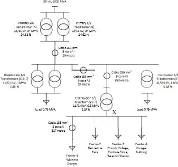
The network topology used for the implementation of the model-based analysis method is shown in Figure 1 below, which is based on a part of the distribution net-work in central Glasgow. The modelled netnet-work consists of an 11 kV and an LV network with fault levels of 250 MVA and 25 MVA, respectively. The LV network is composed of four feeders fed by the distribution substation (S/S) F. One of the four feeders supply the inductive wireless charger, while the other three feeders sup-ply a mix of load which is largely residential and commercial.

The electrical data for the transformers is provided inTable 3while Table 4 lists cable parameters.

Table 3: Network transformer details

Transformer Type Identifier

Voltage [kV]

Power [MVA]

Impedance [%]

Primary A, B 33/11 12/24 24.62

Distribution C, D, E 11/0.4 1 4.88

Distribution F 11/0.4 0.5 5.07

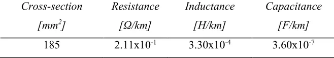
Table 4: Characteristics of the 3-core Aluminium cable modelled in simulation

Cross-section [mm2_]

Resistance [Ω/km]

Inductance [H/km]

Capacitance [F/km]

185 2.11x10-1 _3.30x10-4 _3.60x10-7

3 METHOD

The network shown in Figure 1 is modelled in SIMULINK using standard trans-former blocks and 3-phase PI sections to simulate conductor lengths between the transformers and measurement point. When the properties of the physical network have been adequately represented, the next stage is to attempt to recreate a real phys-ical measurement taken at point X with an Outram Power Quality Analyser [9]. This is done by simulating the model with a HV supply at fundamental frequency and additional sources of voltage harmonics and current harmonics, which can be tuned to match the observed distortion at the measurement point. The method by which the distortion can be retrospectively added to the model has been described in a pre-vious publication [1]. This involves calculating the magnitude and phase shift in-duced by the network components, in a harmonic source voltage and current, where these parameters are known. The difference between the harmonic source and what is seen at the measurement point is a complex quantity representing the magnitude and phase difference. Therefore, the ratio between the source values and the meas-urement point values for each harmonics considered in this study can be defined as a set of complex coefficients, which transform the harmonic source values to the measurement point values, and vice versa. In short, the method aims to use the SIMULINK model to first establish these coefficients in the most effective manner possible and then use them on a measured waveform in order to create the harmonic voltage and current sources necessary to reconstruct the measurement. The benefit of using this approach is that another harmonic source can be added at any point in the network and by the principle of wave superposition, its effect can be accurately modelled at the measurement points in the SIMULINK model.

3.1 SIMULINK

3.2 Complex amplitude transfer coefficients

The modification made here to the method previously proposed in [1] for calculating the complex transfer coefficients is to automate the process using fast Fourier trans-form (FFT) analysis. Harmonic frequency components of a wavetrans-form are a complex quantity with a magnitude and phase. Therefore, the ratio of the measured harmonic signal to the harmonic input source at the same frequency, defines the transfer coef-ficient, which is the same complex quantity described in [1].

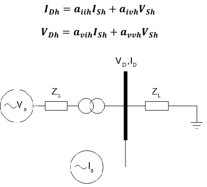
𝑰_𝑫𝒉= 𝒂_𝒊𝒊𝒉𝑰_𝑺𝒉+ 𝒂_𝒊𝒗𝒉𝑽_𝑺𝒉 (1)

𝑽_𝑫𝒉= 𝒂_𝒗𝒊𝒉𝑰_𝑺𝒉+ 𝒂_𝒗𝒗𝒉𝑽𝑺𝒉 (2)

Figure 2: Definition of the voltage and current quantities in the network.

This is defined in equations (1) and (2), where the subscript D indicates a measured quantity, h denotes a particular harmonic frequency, S corresponds to a harmonic source, 𝑎 is a complex transfer coefficient with its subscript indicating that it repre-sents the relationship between corresponding measured quantity (first letter) and source quantity (second letter). For example, 𝑎_𝑖𝑖ℎ is a complex number representing the ratio between the measured current and source current at a particular harmonic frequency ℎ. One can also see from equations (1) and (2) that there is an interde-pendence between voltage and current measurements and their harmonic sources.

3.3 Coefficient Determination

is to perform two simulations. Firstly with 𝑉_𝑠= 0, this simulation allows the calcu-lation of 𝑎_𝑖𝑖ℎ and 𝑎_𝑣𝑖ℎ from equations (1) and (2) directly. Then with 𝐼_𝑠 = 0, the same calculation returns 𝑎_𝑣𝑣ℎ and 𝑎_𝑖𝑣ℎ.

A separate FFT analysis of the harmonic source and measurement point waveforms created by the SIMULINK model, allows the ratio of the FFT complex-valued output arrays created by the FFT MATLAB function to be used for calculating the coeffi-cient values over the entire frequency range of the FFT array.

Therefore, at harmonic frequency ℎand with 𝑉_𝑠 = 0, the coefficient 𝑎_𝑖𝑖ℎ can be cal-culated as:

𝒂𝒊𝒊𝒉= 𝑭𝑭𝑻(𝒊𝑫𝒉)/𝑭𝑭𝑻(𝒊𝑺𝒉) (3)

4 RESULTS

To demonstrate the method, the simulation model was run using a set of harmonics with equal magnitudes to allow the calculation of the coefficients. Following this, the coefficients are used on the measured data to calculate the harmonic voltage and current sources that would be needed to reproduce this measurement in the model. Then an extra 3-phase harmonic source is introduced at the LV side of the model, imitating the effect of an inductive charger used for wireless charging of electric vehicles in this case.

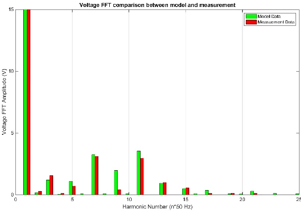
Figure 3: Comparison of the measured and reconstructed voltage at the

measure-ment point. The triplen harmonics of 9 and 21 show a significant disagreemeasure-ment from measurement, and investigation of this will be part of further investigations in the future.

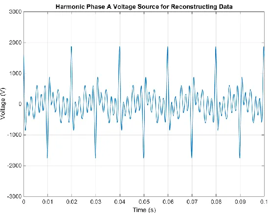
Figure 4: Harmonic Voltage source used to recreate the measured LV quantities.

Figure 5 shows the harmonic components of the real current measurement and the modelled values.

Figure 5: A comparison of the harmonic current components measured by the

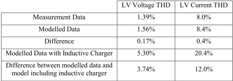
The important result here is the comparison in Table 5 showing the comparison in LV voltage THD value between the measured values and the reconstructed values. The error between measurement and model here is~0.2%.

Table 5: Results comparing measured harmonic parameters and the model results on phase A.

LV Voltage THD LV Current THD

Measurement Data 1.39% 8.0%

Modelled Data 1.56% 8.4%

Difference 0.17% 0.4%

Modelled Data with Inductive Charger 5.30% 20.4% Difference between modelled data and

model including inductive charger 3.74% 12.0%

After injecting the distorted waveform associated with the inductive charger into the model, Table 5 also shows the observed increase in voltage and current THD at the model measurement point.

It can be seen that the inductive charger causes a large increase in the LV Voltage THD as observed at the measurement point.

The modelled increase in THD of the LV voltage supply actually exceeds the speci-fied limits of the G5/4-1 recommendations here, and since the agreement between model and measurement is fairly good, it is possible to identify the main source of this extra distortion.

Figure 6: FFT analysis of the Inductive Charger harmonic current components

which are injected into the model.

5 CONCLUSION

This paper demonstrates the potential of an extension to the method described in [1] for approaching a synthetic reconstruction of harmonic sources present in a power network, which allows the use of modelling software like SIMULINK to calculate the impact on the network from adding other sources of harmonic distortion. A method has been demonstrated which builds upon previous work to automate the creation of a table of coefficients which allows the recreation of distorted voltage and current from real network data.

This method is aimed at analysing the grid compliance and network effect of the expected surge in distributed generation and electric vehicles in the future develop-ment of smart grids.

6 FUTURE WORK

It has been observed that the attenuation of the triple harmonics (h=3, 9, 15…) which is expected in a delta-star transformer, is not properly represented in this SIMULINK model. This does not significantly affect the calculation of THD shown in Table 5, however this issue will be investigated in detail in future applications of this model. Extending the scope of the case study for different network configurations and a variety of transformer will also be a priority in future model applications

7 REFERENCES

[1] A. Dysko, G. Burt, J. McDonald and J. Clark, “Synthesis of Harmonic Distortion Levels in an LV Distribution Network,” IEEE Power Engineering Review, vol. 21, no. 5, pp. 58-60, 2001.

[2] G5/4-1, Engineering Recommendation, Planning Levels For Harminc Voltage Distortion And The COnnection Of Non-Linear Equipment To Transmission Systems And Distribution Networks In The UK, Energy Networks Association, 2005.

[3] BS EN 61000-3-2:2006+A2:2009, Part 3.2: Limits for harmonic current emissions (equpiment input current ≤ 16A per phase), British Standards Institution, 2006.

[4] BS EN 61000-3-12:2005, Part 3-12: Limits for harmonic currents produced by equipment connected to public low-voltage systems with input current >16 A and <75 A per phase, British Standards Institution, 2005.

[5] A. Dysko, G. Burt and J. McDonald, “Assessment of Harmonic Distortion Levels in LV Networks With Increasing Penetration Levels Of Inverter Connected Embedded Generation,” in CIRED, 18th International Conference on Electricity Distribution, Turin, 2005.

[6] I. Santos and V. e. a. Cuk, “Considerations on hosting capacity for harmonic distortions on transmission and distribution systems,” Electric Power Systems Research, vol. 119, no. February, pp. 199-206, 2015.

the harmonic voltage distortions in urban distribution systems,” Renewable Energy, vol. 76, no. April, pp. 454-464, 2015.

[8] K. McBee and M. Simoes, “Evaluating the Long-Term Impact of a Continuously Increasing Harmonic Demand on Feeder-Level Voltage Distortion,” IEEE Transactions on Industry Applications, vol. 50, no. 3, pp. 2142-2149, 2014.