A spin chain model with non-Hermitian interaction: the Ising quantum spin chain in an imaginary field

City, University of London Institutional Repository

Citation:

Castro-Alvaredo, O. and Fring, A. (2009). A spin chain model with non-Hermitian interaction: the Ising quantum spin chain in an imaginary field. Journal of Physics A:

Mathematical and Theoretical, 42(46), doi: 10.1088/1751-8113/42/46/465211

This is the unspecified version of the paper.

This version of the publication may differ from the final published

version.

Permanent repository link:

http://openaccess.city.ac.uk/765/

Link to published version:

http://dx.doi.org/10.1088/1751-8113/42/46/465211

Copyright and reuse: City Research Online aims to make research

outputs of City, University of London available to a wider audience.

Copyright and Moral Rights remain with the author(s) and/or copyright

holders. URLs from City Research Online may be freely distributed and

linked to.

arXiv:0906.4070v2 [hep-th] 1 Jul 2009

A spin chain model with non-Hermitian interaction:

The Ising quantum spin chain in an imaginary field

Olalla A. Castro-Alvaredo and Andreas Fring

Centre for Mathematical Science, City University London, Northampton Square, London EC1V 0HB, UK

E-mail: O.Castro-alvaredo@city.ac.uk, A.Fring@city.ac.uk

Abstract: _{We investigate a lattice version of the Yang-Lee model which is}

character-ized by a non-Hermitian quantum spin chain Hamiltonian. We propose a new way to implementPT-symmetry on the lattice, which serves to guarantee the reality of the spec-trum in certain regions of values of the coupling constants. In that region of unbroken

PT-symmetry we construct a Dyson map, a metric operator and find the Hermitian counterpart of the Hamiltonian for small values of the number of sites, both exactly and perturbatively. Besides the standard perturbation theory about the Hermitian part of the Hamiltonian, we also carry out an expansion in the second coupling constant of the model. Our constructions turns out to be unique with the sole assumption that the Dyson map is Hermitian. Finally we compute the magnetization of the chain in the zandxdirection.

1. Introduction

It is known for about thirty years that ordinary second order phase transitions can be described by the Yang-Lee model [1, 2, 3]. This model admits a quantum field theoret-ical description in form of a Landau-Ginzburg Hamiltonian for a scalar field φ with an additional φ3-interaction and a term linear in the scalar field with an imaginary coupling constant. The model has been identified [4] as a perturbation of the _M5,2-model in the

Mp,q-series of minimal conformal field theories [5]. It is the simplest non-unitary model

in this infinite class of models, which are all characterized by the conditionp₋q >1 and whose corresponding Hamiltonians are all expected to be non-Hermitian.

Here we shall investigate a discretised lattice version of the Yang-Lee model considered by von Gehlen [6, 7], which is an Ising quantum spin chain in the presence of a magnetic field in the z-direction as well as a longitudinal imaginary field in the x-direction. The corresponding Hamiltonian for a chain of length N is given by

H(λ, κ) =₋1 2

N

X

j=1

It acts on a Hilbert space of the form (C2₎⊗N _{where we employed the standard notation for}

the 2N_×2N-matricesσx,y,z_i =I_⊗I_{⊗. . .⊗σ}x,y,z_{⊗. . .⊗}I_⊗I_{with Pauli matrices describing}

spin 1/2 particles

σx = 0 1

1 0

!

, σy = 0 −i

i 0

!

, σz = 1 0

0 ₋1

!

, (1.2)

asith factor acting on the siteiof the chain. Their commutation relations are direct sums of su(2) algebras

[σx_j, σy_k] = 2iσz_jδjk, [σzj, σxk] = 2iσ y

jδjk, [σyj, σzk] = 2iσxjδjk, withj, k = 1, . . . , N (1.3)

A further real parameterβmay be introduced into the model by allowing different types of boundary conditions σx,y,z_N+1=βσx,y,z₁ , albeit here we will only consider the case of periodic boundary conditions and takeβ = 1.

Since all Pauli matrices are Hermitian it is obvious thatH(λ, κ) is non-Hermitian

H†(λ, κ) =H(λ,₋κ)₆=H(λ, κ). (1.4)

This poses immediately two questions: First of all, is the spectrum still real, despite the fact that the vital property of Hermiticity which guarantees this is given up and second is it still possible to formulate a meaningful quantum mechanical description associated to this type of Hamiltonians? These issues have attracted a considerable amount of attention in the last ten years, since the seminal paper by Bender and Boettcher [8] and meanwhile many satisfying answers have been found to most of them; for recent reviews see [9, 10, 11]. Our manuscript is organised as follows: In section 2 we present various alternatives about how _PT-symmetry can be implemented for quantum spin chains. In section 3 we establish our notation and recall some of the well known facts concerning a consistent quantum mechanical framework for _PT-symmetric systems. We analyze the model (1.1) in section 4 and section 5, where the former is devoted to non-perturbative and the latter to perturbative results. In section 6 we compute the magnetization for the model (1.1) and we state our conclusions in section 7.

2. _PT-symmetry for spin chains

Preceding the above mentioned recent activities von Gehlen found numerically [6, 7] that for certain values of the dimensional parametersλand κthe eigenvalues forH(λ, κ) are all real, whereas for the remaining values they occur in complex conjugate pairs. He provided an easy explanation for this feature: Acting adjointly on the Hamiltonian with a spin rotation operator

R=eiπ4S

N z ₌

N

Y

i=1

1 √

2(I+iσ

z₎

i, with SzN = N

X

i=1

σz_i, I₌ 1 0

0 1

!

, (2.1)

has the effect of rotating the spins at each site clockwise byπ/2 in thexy-plane, such that the corresponding map acts as_R: (σx

is a 2N _×2N _{non-symmetric matrix with real entries given by}

ˆ

H(λ, κ) =_RH(λ, κ)_R−1₌₋1

2

N

X

i=1

(σz_i +λσy_iσy_i+1−iκσy_i). (2.2)

Its eigenvalues and those ofH(λ, κ) are therefore either all real or occur in complex conju-gate pairs. This is precisely the well known behaviour one finds whenH(λ, κ) is symmetric with respect to an anti-linear operator [12, 13, 14, 15, 16], which as mentioned above has recently attracted a lot of attention. In quantum mechanical or field theoretical models the anti-linear operator is commonly taken to be the _PT-operator, which carries out a simul-taneous parity transformation_P :x_{→ −}x and time reversal_T :t_{→ −}t. When acting on complex valued functions the anti-linear operator_T is understood to act as complex con-jugation. Real eigenvalues are then found for unbroken_PT-symmetry, meaning that both the Hamiltonian and the eigenfunctions remain invariant under _PT-symmetry, whereas broken _PT-symmetry leads to complex conjugate pairs of eigenvalues.

We will now argue that _PT-symmetry on the lattice can be interpreted in various ways. One may for instance reflect the chain across its midpoint via the map_P′ _:σx,y,z

i →

σx,y,z_N+1−i as suggested by Korff and Weston [17] and used thereafter in [18]. It is obvious that the Hamiltonian (1.1) is invariant with regard to this symmetry. However, when keeping the interpretation of_T as a complex conjugation, and thus ensuring that the_P′_T

-operator is anti-linear, one easily observes that this type of transformation does not leave the Hamiltonian (1.1) invariant, i.e. we have [_P′_T, H]₆= 0.

Therefore we need to implement _PT-symmetry in a different way for H(λ, κ) to be able to analyze its properties along the lines proposed in [12, 13, 14, 15, 16]. We propose here that one carries out a parity transformation at each individual site and reflect every spin for instance in the xy-plane on y = ₋x. This is obviously achieved by _R2_{. As}

R4=QN

i=1(−I)i = (−1)NI⊗N and not the desired identity operator, we take here

P =₋i_R2 =eiπ2(S

z₋

I)₌

N

Y

i=1

σz_i, with _P2=I⊗N_{, (2.3)}

as our parity operator. Consequently this transformation acts as

P : (σx_i, σy_i, σz_i)_→(₋σx_i,₋σy_i, σz_i). (2.4)

Thus with _T being the usual complex conjugation, which acts on the Pauli matrices as

T : (σx_i, σy_i, σz_i)_→(σx_i,₋σy_i, σz_i), (2.5)

we have identified an anti-linear operator constituting a symmetry of the Hamiltonian (1.1)

[_PT, H] = 0. (2.6)

eigenvalues. We can precisely separate the two domains UPT and UbPT in the parameter

space ofλand κ defined by the action on the eigenstates Φ(λ, κ) ofH(λ, κ)

PTΦ(λ, κ)

(

= Φ(λ, κ) for (λ, κ)_∈UPT

6

= Φ(λ, κ) for (λ, κ)_∈UbPT.

(2.7)

According to the general reasoning provided in [12, 13, 14, 15, 16], simultaneous eigenfunc-tions of_PT andH(λ, κ), that is for (λ, κ)_∈UPT, are then associated with real eigenvalues

whereas in the regime of broken _PT-symmetry, that is (λ, κ) _∈ UbPT, the eigenvalues

emerge in complex conjugate pairs.

From the above it is clear that we may define equally well different types of _PT -operators closely related to the one introduced in (2.3). For instance we can define

Px:= N

Y

i=1

σx_i and _Py :=

N

Y

i=1

σy_i, (2.8)

which obviously act as

Px : (σxi, σyi, σzi)→(σxi,−σyi,−σzi) and Py : (σxi, σyi, σzi)→(−σxi, σyi,−σzi). (2.9)

Clearly these parity operators can not be used in the same way as_P in (2.3) to introduce a _PT-symmetry for H(λ, κ) when keeping _T unchanged. However, they serve to treat non-Hermitian Hamiltonians of a different kind, such as obvious modifications of H(λ, κ) and also to allow for alternative treatments of non-Hermitian spin chains, such as the XXZ-spin-chain in a magnetic field [19]

HXXZ =

1 2

N−1

X

i=1

(σx_iσx_i+1+σy_iσ_iy₊₁+ ∆+(σziσzi+1−1)

+∆− 2 (σ

z

1−σzN), (2.10)

with ∆± = (q±q−1)/2 previously studied in [17, 18]. Obviously when q /∈R this

Hamil-tonian is non-Hermitian, but we observe that it is _PT-symmetric when using any of the parity operators defined in (2.8) and keeping_T to be the usual complex conjugation

[_PxT, HXXZ] = 0 and [PyT, HXXZ] = 0. (2.11)

Thus besides reflecting the chain across its midpoint in form of a “macro-reflections”, as suggested in [17], we may also carry out the parity transformations on each individual side. It appears that these “micro-reflections” (2.3), (2.8) allow for a wider range of possibilities, such as for instance Hamiltonians of the typeH(λ, κ) in (1.1), which could not be tackled with _P′ : σx,y,z_{i →} σx,y,z_N+1−i. The different possibilities are simply manifestations of the well known ambiguities non-Hermitian Hamiltonians possess with regard to their operator content [21]. This also means that the symmetries (2.11) will lead to a different kind of physical systems than those identified in [17].

It is well known that HXXZ can be expressed in terms of generators of a

It is then trivial to see that the algebra remains invariant under a_PT-transformation when realized as (2.8): _T :Ei → Ei∗,Px,y :Ei → Ei∗, such that Px,yT :Ei →Ei. On the other

hand when implementing the “macro-reflection” on the entire chain, the _P′_T-symmetry

on the generators is broken, i.e. _P′_T :Ei→EN+1−i, as was found in [17].

A further interesting non-Hermitian quantum spin chain has recently been investigated by Deguchi and Ghosh [20]

HDG=

N

X

i=1

κzzσziσzi+1+κxσxi +κyσyi, (2.12)

with κzz ∈ R and κx, κy ∈ C. Clearly when κx or κy ∈/ R the Hamiltonian HDG is

not Hermitian, which is the case we will consider. As the previous model also the quasi-Hermitian transverse Ising model allows for different types of realizations for the _PT -symmetry. We easily observe that the macro-reflections can not be implemented

P′T, H

6

= 0, (2.13)

whereas all the micro-reflections can be realized

[_PT, H] = 0 forκx, κy ∈iR,

Px/yT, H

= 0 forκ_x/y∈R_{, κy/x ∈i}R_{. (2.14)}

Once again these different possibilities raise the question about the unique of the operator content in the model.

Having an explanation for the nature of the eigenvalue spectra, it is left to show that one may in addition construct a meaningful metric for this Hamiltonian with well defined quantum mechanical observables associated to it. As already indicated, the metric is not even expected to be unique so that, unlike as for the Hermitian case, the observables are no longer defined by the Hamiltonian alone [21]. It remains therefore ambiguous what Hamil-tonians of the type H(λ, κ) describe in terms of physical observables. Having constructed a metric one may often also compute an isospectral Hermitian counterpart forH(λ, κ) for which the physical observables have the standard meaning.

One of the main purposes of this manuscript is that of finding the Hermitian coun-terparts of the Hamiltonian (1.1) and studying in some detail (at least for small N) how many such Hermitian Hamiltonians can be constructed.

3. Generalities

3.1 A new metric and an isospectral Hermitian partner from _PT-symmetry

For the sake of self-consistency, we briefly recall the well known procedure [12, 13, 14, 15, 16] of how to construct a meaningful metric and isospectral Hermitian counterpart, h, for a non-Hermitian Hamiltonian, H. We assume the Hamiltonian to be diagonalizable and to possess a discrete spectrum. Being non-Hermitian the Hamiltonian has non identical left |Φ_i and right eigenvectors _|Ψ_i with eigenvalue equations

The eigenvectors are in general not orthogonal_hΦn|Φmi 6=δnm, but form a biorthonormal

basis

hΨn|Φmi=δnm,

X

n

|Ψni hΦn|=I. (3.2)

We assume the existence of a selfadjoint, but not necessarily positive, parity operator _P whose adjoint action conjugates the Hamiltonian

H†=_PH_P with _P2 =I_{. (3.3)}

The action of this operator on the eigenvectors

P |Φni=sn|Ψni withsn=±1 (3.4)

defines the signatures= (s1, s2, . . . , sn), which serves to introduce the so-calledC-operator1

C:=X

n

sn|Φni hΨn|, (3.5)

satisfying

[_C, H] = 0, [_C,_PT] = 0, _C2=I_{. (3.6)}

Next we employ this operator to define a new operatorρ, which also relates the Hamiltonian to its conjugate

ρ:=_PC, H†ρ=ρH. (3.7)

Depending now on the assumptions made for ρ, such systems allow for different types of conclusions. When ρ is positive and Hermitian, but not necessarily invertible, the system is referred to as quasi-Hermitian [22, 21]. In this case the existence of a definite metric is guaranteed and the eigenvalues are real. In turn when ρ is invertible and Hermitian, but not necessarily positive, the system is called pseudo-Hermitian [23, 24, 25]. For this type of scenario the eigenvalues are always real but no definite conclusions can be made with regard to the existence of a definite metric. Here we will identify operators ρ which are quasi-Hermitian as well as pseudo-Hermitian.

Finally we may factorizeρinto a new operator2 ηand use it to construct an isospectral Hermitian counterpart for H

h=ηHη−1 =h† _⇔ H†=ρHρ−1 withρ=η†η. (3.8)

In other words assuming the existence of an inverse for ρ and its factorization in form of (3.8) one can derive a Hermitian counterpart hforH and vice versa.

1

The is an unfortunate notation and it should be pointed out that the operator is not related to the standard charge conjugation operator in quantum field theory.

2_When

η is Hermitian, it just corresponds to a Dyson transformation [26] employed in the so-called

Holstein-Primakov method [27]. For practical purposes it is useful to have a name for this operator and

3.2 Expectation values of local observables

As discussed above, when dealing with non-Hermitian Hamiltonians the standard metric is generally indefinite and therefore a new, physically sensible, metric needs to be defined by means of the construction described before. This amounts to introducing a new inner product_{h | i}ρ which is defined in terms of the standard inner producth | ias

hΦ_|Ψ_iρ:=hΦ|ρΨi, (3.9)

for arbitrary states,_hΦ_|and_|Ψ_i. Assuming that all local operators_Oin the non-Hermitian theory are related to their counterparts o in the Hermitian theory in the same manner as the corresponding Hamiltonians

η_Oη−1 =o, (3.10)

one finds that a generic matrix element of the operator_O has the form,

hΦ_|ρ_O|Ψ_i=_hΦ_|η†oη_|Ψ_i=_hφ_|o_|ψ_i, (3.11)

where _|Ψ_i and _hΦ_| are eigenstates of the non-Hermitian Hamiltonian and its conjugate, respectively. The states_|ψ_iand_hφ_|are related to the previous two states by_|ψ_i=η_|Ψ_iand hφ_|=_hΦ_|η†, that is, they are eigenstates of the Hermitian Hamiltonian corresponding to the same eigenvalues. Equation (3.11) will be used later on in this paper for the computation of various kinds of expectation values.

3.3 Perturbation theory

In most cases the above mentioned operators can not be computed exactly and one has to resort to a perturbative analysis. Let us recall the main features of such a treatment. To start with it is convenient to separate the Hamiltonian into its Hermitian and non-Hermitian part as H(λ, κ) = h0(λ) +iκh1, where h0 and h1 are both Hermitian with κ

being a real coupling constant. The latter term may then be treated as the perturbing term. For our concrete case (1.1) the individual components are

h0(λ) =−1

2

N

X

i=1

(σz_i +λσx_iσ_ix₊₁), and h1 =−1

2

N

X

i=1

σx_i, (3.12)

such that h0(λ) corresponds to the Ising spin chain coupled to a magnetic field in the z

direction and the perturbing term is an imaginary magnetic field in the x-direction. In order to determineη,ρ and h we can now solve either of the two equations in (3.8). Here we decide to commence with the latter. Making the further assumption thatηis Hermitian and of the formη =eq/2 _{this amounts to solving}

H†=eqHe−q=H+ [q, H] +1

2[q,[q, H]] + 1

3![q,[q,[q, H]]] +· · · (3.13)

where we have employed the Backer-Campbell-Hausdorff identity. Writing H and H† _in

terms ofh0 and h1 equation (3.13) becomes

2iκh1+iκ[q, h1] +

iκ

2[q,[q, h1]] +· · ·= [h0, q] + 1

For most non-Hermitian Hamiltonians, such as for our model (1.1), this equation is very difficult to solve forq. When the (ℓ+1)-fold commutator ofqwithh0, denoted byc(qℓ+1)(h0)

vanishes, closed formulae were found in [28]

h=h0+ [ℓ

2]

X

n=1

(₋1)nEn

4n_(2n)! c

(2n)

q (h0), H =h0− [ℓ+1

2 ]

X

n=1

κ2n−1

(2n₋1)!c

(2n−1)

q (h0), (3.15)

where [x] denotes the integer part of a numberxand Enare Euler’s numbers, e.g. E1 = 1,

E2 = 5, E3 = 61, E4 = 1385, . . . The coefficients κ2n−1 were determined by means of a

recursive equation, which was solved by

κn=

1 2n

[(n+1)/2]

X

m=1

(₋1)n+m

n

2m

Em, (3.16)

such thatκ1 = 1/2, κ3 =−1/4, κ5 = 1/2, κ7 =−17/8, . . .

One may also impose some further structure onq and expand it as

q =

∞

X

k=1

κ2k−1q2k−1, (3.17)

so that each perturbative contribution q2k−1 is a κ-independent matrix. For models of the

form considered here only odd powers of κ appear in the perturbative expansion. This is essentially due to the fact thatHandH†are related to each other byκ_{→ −}κ. Substituting the expansion (3.17) into the equation (3.14) one finds a set of equations for q1, q3, q5, . . .

by equating those terms in (3.14) which are of the same order in perturbation theory inκ. The first few equations are given by

[h0, q1] = 2ih1, (3.18)

[h0, q3] =

i

6[q1,[q1, h1]], (3.19)

[h0, q5] =

i

6[q1,[q3, h1]] +

i

6[q3,[q1, h1]]−

i

360[q1,[q1,[q1,[q1, h1]]]]. (3.20)

As we can see easily, they can be solved recursively, namely onceq1is known, one case solve

forq3 and so on. A closed expression for the commutator [h0, qn] in terms of commutators

[qm, h1] with m < n was derived in [18]. Perturbation theory has been carried out in the

past for various non-Hermitian models, e.g. [16, 28, 29, 30, 31, 18].

The model at hand is special in the sense that it involves two coupling constants, i.e. κ and λ, such that it allows for an alternative perturbative expansion in terms of the latter. Indeed we will demonstrate below that the caseλ= 0 can be solved exactly and we can therefore expand around that solution. Proceeding similarly as for theκ-perturbation theory we separate the Hamiltonian into its single spin contribution and into the nearest neighbour interaction term H(λ, κ) = ˜H0(κ) +λ˜h1with

˜

H0(κ) =−

1 2

N

X

i=1

(σz_i +iκσx_i) and h˜1=−

1 2

N

X

i=1

We stress that the counterparts of (3.18)-(3.20) in the well known κ-expansion explained above differ substantially in the λ-expansion. The details will be explained in the main part of the manuscript below. Having the option to construct two perturbative series, we in principle have in addition the possibility to combine them in a manner that has proved to be very successful in the context of high intensity laser physics [32].

3.4 Ambiguities in the physical observables

As mentioned previously, one can argue that the metricρis not unique. In the perturbation theory framework, this can be easily seen from the fact that the equations (3.18)-(3.20) (and any other equations arising at higher orders in perturbation theory) admit many different solutions. The non-uniqueness of η or, equivalently, the fact that several independent Hermitian Hamiltonians h may exist which are all related to the same non-Hermitian Hamiltonian by different unitary transformations is well known in the literature. Indeed, this fact has been noticed already in the past [21, 33, 30, 34, 35, 36] and is currently still object of debate [37, 38].

Assuming now the Dyson mapη in (3.8) to be Hermitian and related to the operators P,_C and ρas defined in (3.7) we simply obtain

η=η† _⇒ η2 =ρ=_PC. (3.22)

Writing η =eq/2, it is obvious that we can always add to q any matrix b that commutes with the full Hamiltonian [H, b] = 0 and withq, [q, b] = 0

h=eq/2+bHe−q/2−b =eq/2He−q/2, (3.23)

and still solve equations (3.8). This kind of ambiguity is not very interesting, as it will not change h and therefore not lead to new physics. A somewhat less trivial ambiguity was pointed out in [30], which will generate different types of Hermitian counter-parts toH. It originates from the fact that we can always add toq1, q3, q5, . . .any matrix commuting with

h0 as we may easily observe in equations (3.18)-(3.20). Below we will see that in principle

for specific examples many such matrices can be found.

However, by relatingηto the operators_Cand_P as in (3.22) we are introducing further constraints on the form ofη. These constraints follow from the equations (3.6), particularly the last two equations there. Using the explicit form (3.22) they can be rewritten as

PTeq_PT =eq, _Peq_P =e−q. (3.24) by employing the equality_C=η2_P =eq_P. In order for (3.24) to be satisfied, it is required that

Pq_P =_Tq_T =₋q, (3.25)

and consequently

Pq2k−1P =Tq2k−1T =−q2k−1, ∀ k∈Z+. (3.26)

Below, we will show that these constraints are sufficient in many cases to fix the operatorη

4. The Yang-Lee quantum chain: non perturbative results

We will now employ the general ideas and definitions introduced in the previous subsection for the quantum spin chain Hamiltonian (1.1). In particular, we will show how to obtain exact solutions for the operatorsη,ρ and h in the two particular situations: i) λorκ are vanishing andN is generic and ii)λand κ are arbitrary and N is taken to be small.

For large values ofN it will be convenient to use the following abbreviation

S_aN1a2...ap:=

N

X

k=1

σa1

k σ a2

k+1. . . σ

ap

k+p−1, for ai =x, y, z, u; i= 1, . . . , p≤N. (4.1)

We denote hereσu _{=I to allow for non-local, i.e. not nearest neighbour, interactions. In}

this notation the Hamiltonian (1.1) reads

H(λ, κ) =h0(λ) +iκh1, with h0(λ) =−

1 2(S

N

z +λSxxN), h1 =−

1 2S

N

x . (4.2)

In what follows it will also be important to use the adjoint action of_P,_T and_PT on the generatorsS_aN_1a2...ap. It is easy to compute

PS_aN_1a2...apP = (₋1)ny+nx_SN

a1a2...ap, (4.3)

TS_aN_1a2...apT = (₋1)ny_SN

a1a2...ap, (4.4)

PTS_aN_1a2...apPT = (₋1)nx_SN

a1a2...ap, (4.5)

where nx, ny are the numbers of indices ai equal to x, y, respectively. These identities

follow directly from the definitions (2.4) and (2.5).

4.1 Limiting cases: λ= 0 or κ= 0

Let us start by considering the special case λ= 0 for which

h0(0) =−

1 2S

N

z and h1=−

1 2S

N

x . (4.6)

Although the Hamiltonian is extremely simple, it is still non-Hermitian, and thus serves as a benchmark to illustrate the above mentioned notions. For example, a matrix η that relates H(0, κ) to its Hermitian counterparth(0, κ) is easily found to be

η=eq/2 =e−12arctanh(κ)S

N

y _{. (4.7)}

Its adjoint action onSN_x and S_zN is simply

ηS_xNη−1= _√ 1

1₋κ2(iκS

N

z +SxN), ηSzNη−1=

1 √

1₋κ2(S

N

z −iκSxN), (4.8)

which when we evaluate (3.8) yields the Hermitian counterpart to ˜H0(κ) in (3.21)

h(0, κ) =₋1 2

p

1₋κ2_SN

This Hamiltonian describes a spin chain for which no mutual interaction between spins along the chain occurs. An external magnetic field is applied at each site of the chain, whose intensity is governed by the value ofκ and is the same at every site. The constraint −1< κ <1 ensures the Hamiltonianh(0, κ) andηto be Hermitian. Given the simplicity of

h(0, κ) we can easily find its full set of eigenstates and eigenvalues, hence those ofH(0, κ). The operator SN

z is a diagonal matrix with entries

S_zN = diag(N, N ₋2, . . . ,₋N + 2,₋N). (4.10)

The entries in the diagonal (eigenvalues) areN₋2pwithp= 0, . . . , N. They are not neces-sarily in decreasing order and, except forN and₋N, all other eigenvalues are degenerate. For example, the eigenvaluesN₋2 and 2₋N are alwaysN times degenerate. This means that there is a single ground state with minimum energy,

Eg(κ) =− N

2

p

1₋κ2_{, (4.11)}

and the corresponding eigenstate is simply

|ψ_gi=

N

O

i=1

1 0

!

i

, (4.12)

associated to a configuration with all spins “up”, hence aligned with the magnetic field that is being applied at each site of the chain.

The situation whenκ = 0 andλis arbitrary corresponds to the Hermitian Hamiltonian given by h0(λ), that is the Ising spin chain with a magnetic field in the z-direction. In

this case, η = I_{, which is automatically ensured when using perturbation theory. The}

eigenstates and eigenvalues of this Hamiltonian have been studied in the literature by using the Bethe ansatz approach, see e.g. [39, 40]. In particular, the ground state can not be written in such as simple form as (4.12), as it will depend on the value ofλ. One does know however, that, for finite N, it will interpolate between theλ= 0 case, in which the ground state is (4.12) and the λ_{→ ∞} case, in which the ground state will correspond to alternating up-down spins.

4.1.1 Uniqueness of the Dyson operator

In light of the discussion in section 3.4 it is also interesting to investigate the uniqueness of (4.7). Indeed, we will now show that (4.7) is the only solution to (3.8) which is consistent with (3.24) for the Hamiltonian H(0, κ). This can be proven in two steps: firstly we will characterize the subset of matrices and linear combinations thereof that satisfy (3.25) and secondly, we will show that none of these matrices can be in the kernel of h0(0). Let us

define the matrices, which provide a basis for the set of 2N _⊗2N-Hermitian matrices,

Ma1...aN =σ

a1

1 ⊗ · · · ⊗σaNN, with ai =x, y, z, oru ∀ i= 1, . . . , N. (4.13)

Recall the definition σu_i = I_{i. Let us consider an arbitrary linear combination of the}

analogous to (4.3) and (4.4). From this it follows that, in order for any linear combination of matrices Ma1,...,ap to transform as q does in equations (3.25) it must be such that for

all matrices in the linear combinationny is odd and nx is even (nx andny as defined after

equation (4.5)).

We will now argue that no matrix in the kernel of h0(0) is of this form. There are

various ways of having a vanishing commutator [h0(0), B] = 0. The most obvious solution

is forB to be a diagonal matrix, ash0(0) is itself diagonal. In terms of the matrices (4.13),

this means selecting out those that are tensor products ofσz and I_{only. There are overall}

2N _{such matrices and obviously none of them has n}

y odd. This would be sufficient to

conclude that the solution (4.7) is unique if only the kernel of h0(0) had dimension 2N.

This is not so because h0(0) has degenerate eigenvalues.

Any additional matrices in the kernel will be some linear combination of matrices (4.13) involving at least one indexxory. Employing the commutation relations (1.3), it is easy to see that there are basically two kinds of additional matrices that are in the kernel of h0(0): firstly, the matrices Mxyu...u−Myxu...u and generalizations thereof , which are

antisymmetric under the exchange of indicesx_↔y and violate the conditionnx even and

secondly, the matrices Mxxu...u+Myyu...u and generalizations thereof, which violate the

conditionny odd and are symmetric under the exchange of indicesx↔y. Generalizations

of these matrices are those obtained by replacing any number of indices u by z and/or permuting indices, as well as other matrices of similar characteristics, such as Mxxxxu...u+ Myyyyu...u+Mxxyyu...u+Myyxxu...uand so on. Since this is more an argument than a proof,

we would like to support it with two examples. ForN = 2

h0(0) = diag(−1,0,0,1), (4.14)

and the kernel has dimensions 6, as one eigenvalue is twice degenerate. It is generated by the matrices

Mxy −Myx, Mxx+Myy, Mzz, Mzu, Muz and Muu=I. (4.15)

ForN = 3 we have that h0(0) has four different eigenvalues, two of which are three times

degenerate,

h0(0) = diag

−3₂,₋1

2,− 1 2,

1 2,−

1 2,

1 2,

1 2,

3 2

, (4.16)

The dimension of the kernel then becomes 20. Its generators are the matrices

Mxyu−Myxu, Mxuy−Myux, Muxy−Muyx,

Mxxu+Myyu, Mxux+Myuy, Muxx+Muyy, Mxyz−Myxz, Mxzy−Myzx, Mzxy−Mzyx,

Mxxz+Myyz, Mxzx+Myzy, Mzxx+Mzyy,

Mzzz, Mzzu, Mzuz, Muzz, Mzuu, Muzu, Muuz, Muuu, (4.17)

As shown before, these examples confirm once more that no element in the kernel ofh0(0)

can fulfill the conditions (3.25) and therefore could not be added toq, whilst fulfilling such conditions. Thus no matrices in the kernel of h0(0) satisfy the conditions (3.25) and the

4.2 The N = 2 case: two sites

We have already identified the _PT-symmetry for the Hamiltonian (1.1) with _P given as specified in (2.3) satisfying (3.3). Let us now take the length of the spin chain to beN = 2 and compute the quantities as outlined in the previous section.

For two sites we may chose without loss of generality the boundary conditions to be periodicσx

N+1=σx1 as any other choice may be achieved simply by a re-definition ofλ. In

this case the Hamiltonian (1.1) acquires the simple form of a non-Hermitian 4_×4-matrix. In order to make notations clear, we will write this matrix here in the various notations introduced so far,

H(λ, κ) = ₋1 2[σ

z_⊗I+I⊗σz_{+ 2λσ}x_⊗σx_+iκ(I⊗σx_+σx_⊗I)],

= ₋1 2[σ

z

1+σz2+ 2λσx1σx2+iκ(σx2 +σx1)],

= ₋1 2[S

2

z +λSxx2 +iκSz2] =−

    

−1 iκ₂ iκ₂ λ iκ

2 0 λ iκ2

iκ

2 λ 0

iκ

2

λ iκ₂ iκ_{2 −}1

    

, (4.18)

where the first line shows the most explicit way of writing the Hamiltonian, the second line shows a simplified version, were the tensor products are omitted and absorbed into theσs as specified after (1.1). The last line uses the notation introduced in (4.1).

0.0 0.5 1.0 1.5 2.0 2.5

0.0 0.2 0.4 0.6 0.8 1.0

U bPT

U

[image:14.612.184.411.414.567.2]

PT

Figure 1: Domains of broken and unbrokenPT-symmetry

At first we shall be concerned with the spectral properties of this Hamiltonian. The two subdomainsUPT andUbPT , as introduced in (2.7), have already been identified numerically

in [6] for spin chain lengths up to N = 19, that is for matrices up to the remarkable size of 524288_×524288. ForN = 2 the eigenvalues for (4.18) are easily computed analytically as the characteristic polynomial factorizes into a third and first order polynomial. The discriminant ∆ of the third order polynomial is computed by

∆ =r2₋q3 with q= 1 9 −3κ

2_{+ 4λ}2_{+ 3}

, r= λ

27 18κ

2_{+ 8λ}2_{+ 9}

The eigenvalues are guaranteed to be real when the discriminant is smaller or equal to zero, such thatUPT is defined as

UPT =

λ, κ: ∆ =κ6+ 8λ2κ4₋3κ4+ 16λ4κ2+ 20λ2κ2+ 3κ2₋λ2₋1_≤0 . (4.20)

The regions UPT and UbPT are depicted in Figure 1, from which we note that in order to

have a real eigenvalue spectrumκ is restricted to take values between 0 and 1, whereasλ

is left unboundedλ_∈[0,_∞).

The four real eigenvalues are then computed to

ε1 =λ, ε2 = 2q

1 2 cos θ

3

−λ3, ε3,4 = 2q

1 2 cos θ

3 +π∓23π

−λ3, (4.21)

where the additional abbreviation θ = arccos r/q3/2

has been introduced. We depict these eigenvalues in Figure 2,

0.0 0.1 0.2 0.3 0.4

-1.0 -0.5 0.0 0.5 1.0

= 0.45202439665

n

1

2

3

4

0.0 0.1 0.2 0.3 0.4 0.5

-1.0 -0.5 0.0 0.5 1.0

= 0.4

n

1

2

3

[image:15.612.88.505.210.426.2]

4

Figure 2: Avoided level crossing: eigenvalues as functions of λ(κ) for fixedκ(λ).

where we observe the typical avoided level crossing behaviour of the eigenvalues as a func-tion of the parameters [41], i.e. the eigenvalues ε3 and ε4 only meet in the exceptional

point when they simultaneously become complex.

For the computations of physical observables, which we will carry out below, it is important to identify the lowest eigenvalue, which turns out to be alwaysε4.

Next we compute the right eigenvectors ofH(λ, κ) to

|Φ1i= (0,−1,−1,0), |Φni= (γn,−αn,−αn, βn), n= 2,3,4, (4.22)

with αn=iκ(λ−εn+ 1), βn =κ2+ 2λ2+ 2λεn and γn=−κ2−2εn2 + 2λ−2λεn+ 2εn.

We verify that left and right eigenvectors are related via a conjugation _|Ψni = hΦn| and

compute the signature as defined in (3.4) tos= (+,₋,+,₋) for the parity operator (2.3). Normalizing the vectors in (4.22) by dividing withN1 =√2,Nn= (2α2n+β2n+γ2n)1/2 for n= 2,3,4 we compute the _C-operator according to (3.5) to

C=

    

C5 −C3 −C3 C4

−C3 −C1−1 −C1 C2

−C3 −C1 −C1−1 C2

C4 C2 C2 2(C1+ 1)−C5

    

where the matrix entries are

C1 = α

2 4 N2 4 − α2 2 N2 2 − α2 3 N2 3 − 1

2, C2 =

α4β4

N2 4 −

α2β2

N2 2 −

α3β3

N2 3

, C3= α_N2γ22 2

+ α3γ3

N2 3 −

α4γ4

N2 4

,

C4 = β_N2γ22 2 +

β3γ3

N2 3 −

β4γ4

N2

4 , C5 =

γ2 2 N2 2 + γ2 3 N2 3 − γ2 4 N2 4. (4.24) We may now verify that_Cindeed satisfied the properties (3.6) upon the use of the identities

C2 =C2C5−C3C4, C3 =C5C3−C2C4−2C1C3, C4=C2C3−C1C4,

1 = 2C₃2+C₄2+C₅2, 0 =C₂2+C₃2+ 2C1(C1+ 1).

(4.25)

Next we compute the metric operator in the form ρ=_PC simply from (2.3) and (4.23) to ρ=     

C5 −C3 −C3 C4

C3 1 +C1 C1 −C2

C3 C1 1 +C1 −C2

C4 C2 C2 2(1 +C1)−C5

     (4.26)

Since iαi, βi, γi ∈ R it follows that C1, iC2, iC3, C4, C5 ∈ R and therefore we conclude

immediately that ρ is Hermitian. To see whether ρ is also positive, as it ought to be, we compute its eigenvalues

y1 =y2 = 1 and y3/4 = 1 + 2C1±2

p

C1(1 +C1). (4.27)

Since C1 >0 all eigenvalues of ρ are obviously guaranteed to be positive.

Next we determine the corresponding eigenstates to

|r1i= (0,−1,1,0), |r2i= (C4,0,0,1−C5),

r_3/4

= (˜γ_3/4,α˜3/4,α˜3/4,β˜3/4) (4.28)

with ˜α_3/4 = y_3/4(C3C4 +C2(−4C1 +C5 −1))/2−C3C4, ˜β3/4 = −C32 −C1 −C1C5 +

C₃2+C1(4C1−C5+ 3)

y3/4 and ˜γ3/4 =C1C4−C2C3+ (C2C3+C1C4)y3/4. Defining now

the matrix U = _{r1, r2, r3, r4}, whose column vectors are the eigenvectors of ρ, we may

take the square root of ρ, such thatη =ρ1/2 _{=U D}1/2_U−1_{, whereD= diag(y}

1,y2,, y3,, y4).

The isospectral Hermitian counterpart ofH results from (3.8) to anXY Z spin chain (with just two sites) in a magnetic field

h(λ, κ) = ηHη−1=U D1/2U−1HU D−1/2U−1 (4.29)

= µ2_xx(λ, κ)S2_xx+µ2_yy(λ, κ)S2_yy+µ2_zz(λ, κ)S_zz2 +µ2_z(λ, κ)S_z2. (4.30)

It is clear that the coefficients µ2_xx, µ2_yy, µ2_zz, µ2_z can be computed explicitly, but the expressions are rather lengthy and we will therefore not present them here. They are all real functions ofλandκ. Their explicit form can be found in appendix A in terms of functions of

λand κ(5.10) which will be introduced in section 5, in the context of perturbation theory. In the next section we wish to compare this exact result with a perturbative expansion. Let us therefore report two numerical examples for some isospectral Hermitian counterpart of H(λ, κ)

h(0.1,0.5) =

    

−0.829536 0 0 ₋0.0606492 0 ₋0.0341687 ₋0.1341687 0 0 ₋0.1341687 ₋0.0341687 0 −0.0606492 0 0 0.897873

and

h(0.9,0.1) =

    

−0.985439 0 0 ₋0.890532 0 ₋0.0094167 ₋0.909417 0 0 ₋0.909417 ₋0.0094167 0 −0.890532 0 0 1.00427

    

. (4.32)

Notice that h23=h32=h22−λ=h33−λ.

We have carried out a similar analysis for the chain with three sites explicitly, albeit the resulting formulae are rather cumbersome to present. In any case for longer chains one has to resort to more sophisticated and less transparent techniques as for instance the Bethe ansatz. Alternatively, we may employ perturbation theory.

5. The Yang-Lee quantum chain: perturbative results

In this section we want to address the problem of obtaining the matricesη,ρ and h from a perturbative analysis as described in section 3.3. We will study theN = 2,3 and 4 cases in detail and draw some conclusions concerning the analytic expressions of η, ρ and h for generic N.

5.1 The N = 2 case: perturbation theory in κ

Despite the fact thatH(λ, κ) is just the 4_×4-matrix (4.18), it is actually not easy to find the matrixq in (3.13) exactly. As discussed in section 3.4, it is clear that the equations (3.18) to (3.20) as well as the equations that would be obtained for higher orders in perturbation theory, admit many solutions. Any solutionq2k−1can be modified by adding a matrix that

commutes with h0(λ). However, not all solutions obtained in this manner would be valid

solutions if the equations (3.24) are to hold. For the particular caseN = 2, we are about to show that these constraints actually select out a unique Hermitian counterpart to the Hamiltonian H(λ, κ). We will start by finding the most general matrixq1(λ) which solves

the identity (3.18). It is quite clear that given one solution q1(λ), any matrix of the form

q1(λ) +B(λ) with [h0(λ), B(λ)] = 0 will also be a solution, so we may start by finding

all such matrices. In this simple case, there are four basic independent solutions to the equation [h0(λ), B(λ)] = 0

B1 =I, B2=S2zz, B3 =Sxx2 +Syy2 and B4 =Sz2−λSyy2 . (5.1)

Since h0(λ) is a 4×4-diagonalizable matrix, with non-degenerate eigenvalues, there can

be at most four independent matrices that commute with it, namely those shown above or combinations thereof. On the other hand, it is clear that any polynomial function of the Hamiltonianh0(λ) would also commute withh0(λ). As the four matrices in (5.1) constitute

a basis, we expect to be able to express any power of h0 as linear combinations of them.

Indeed, we find

h0(λ)2n =

(1 +λ2)n 2 (B1+

1 2B2) +

λ2n

2 (B1− 1

2B2), (5.2)

h0(λ)2n+1 = (1 +λ2)nh0(λ) +

λ(1 +λ2)n_−λ2n+1

forn_∈N_{0. Therefore, the most general solution to the first order equation (3.18) for the}

present model is

q1(λ) =−Sy2−λ(Syz2 +Szy2 ) +

4

X

i=1

fi(λ)Bi, (5.4)

where the fi(λ), i= 1,2,3,4 are arbitrary functions ofλ.

Before we proceed to determine q3(λ) by solving (3.19) let us comment on the

am-biguities and answer the question of whether all solutions (5.4) are compatible with the equations (3.24). Specializing equations (4.3) and (4.4) for the matrices in (5.4) we find

PX_P =_TX_T =₋X, forX=S_y2, S_yz2 , S_zy2 (5.5) whereas

PBiP =TBiT =Bi, fori= 1,2,3,4. (5.6)

These equations imply that the equalities (3.24) can only be satisfied if the functions

fi(λ) = 0 for i= 1,2,3,4. Thus we have selected out a unique solution for q1(λ), namely

q1(λ) =−Sy2−λ(Syz2 +Szy2 ). (5.7)

More generally, the conditions (3.24) together with the properties (4.3) and (4.4) imply that

• any solutionsq2k−1 must be linear combinations of matrices (4.1) with ny odd,

• any solutionsq2k−1 must be linear combinations of matrices (4.1) withny+nx odd,

• or, combining the two conditions above, any solutionsq2k−1 must be linear

combina-tions of matrices (4.1) with ny odd andnx even,

as anticipated in subsection 4.1.1. These conditions then automatically guarantee the validity of the_PT-properties (3.26) for theq2k−1. For N = 2, this singles out the matrices

S2

y andSyz2 =Szy2 in (5.7), so that, even before attempting to solve (3.18) we would already

know that it can only be a linear combination of those two matrices. As indicated above, these constraints apply for all other q2k−1(λ), withk >1 so that we can safely claim that,

at all orders in perturbation theory, the matrices q2k−1(λ) must be linear combinations of

the form,

q2k−1(λ) =a2k−1(λ)Sy2+b2k−1(λ)(S2yz+Szy2 ), (5.8)

where a2k−1(λ), b2k−1(λ) are real functions of λ. In other words, all the terms in the

perturbative expansion of q are linear combinations of the same two matrices. Hence, we can write

eq =eα(λ,κ)Sy2+β(λ,κ)(S2yz+Szy2 )_{, (5.9)}

which, after computing the exponential becomes

      

ρ(λ,κ)2_+ǫ(λ,κ)2_{cosh[2γ(λ,κ)]}

2γ(λ,κ)2 −

iǫ(λ,κ) sinh[2γ(λ,κ)] 2γ(λ,κ) −

iǫ(λ,κ) sinh[2γ(λ,κ)] 2γ(λ,κ) −

δ(λ,κ) sinh2

[γ(λ,κ)]

γ(λ,κ)2

iǫ(λ,κ) sinh[2γ(λ,κ)]

2γ(λ,κ) cosh

2_{γ(λ, κ) sinh}2_{γ(λ, κ)}

−iρ(λ,κ) sinh[22γ(λ,κ)γ(λ,κ)]

iǫ(λ,κ) sinh[2γ(λ,κ)]

2γ(λ,κ) sinh

2_{γ(λ, κ) cosh}2_{γ(λ, κ)}

−iρ(λ,κ) sinh[22γ(λ,κ)γ(λ,κ)]

δ(λ,κ) sinh2_γ(λ,κ)

γ(λ,κ)2

iρ(λ,κ) sinh[2γ(λ,κ)] 2γ(λ,κ)

iρ(λ,κ) sinh[2γ(λ,κ)] 2γ(λ,κ)

ǫ(λ,κ)2_+ρ(λ,κ)2_{cosh[2γ(λ,κ)]}

2γ(λ,κ)2

where

α(λ, κ) =

∞

X

k=0

κ2k+1a2k+1(λ), β(λ, κ) =

∞

X

k=0

κ2k+1b2k+1(λ), (5.10)

and

γ(λ, κ) =pα(λ, κ)2_{+ 4β(λ, κ)}2_{, δ(λ, κ) =α(λ, κ)}2_{−4β(λ, κ)}2_{. (5.11)}

ǫ(λ, κ) =α(λ, κ) + 2β(λ, κ), ρ(λ, κ) =α(λ, κ)₋2β(λ, κ). (5.12)

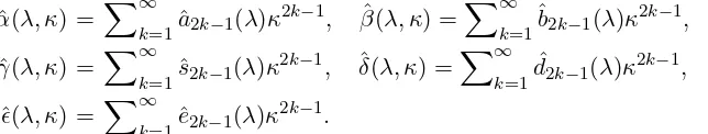
Notice that, for α(λ, κ) and β(λ, κ) real, the matrix above is explicitly Hermitian, as it should be. Once the coefficients α(λ, κ) and β(λ, κ) have been obtained, the Hermitian Hamiltonian (3.8) can be easily computed. The difficulty here is however that general formulae for the coefficientsa2k+1(λ) andb2k+1(λ) are very difficult to obtain. Nonetheless,

perturbation theory allows us to compute these coefficients up to very high orders in powers of κ. In order to solve for such high orders, we have resorted to the use of the algebraic manipulation software Mathematica. It allows us to find the entries of the matrix (5.9) as perturbative series in κ and to fix the coefficients a2k+1(λ) andb2k+1(λ) by matching the

entries of H†_{(λ, κ) and η}2_{H(λ, κ)η}−2_{, order by order in perturbation theory, as expected}

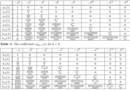
from (3.8). For numerical computations and sufficiently small values ofκthis gives results which are very close to the exact values. In tables 1 and 2 we present the coefficients

a2k+1(λ) andb2k+1(λ) up tok= 7.

−λ0 −λ2 −λ4 −λ6 −λ8 −λ10 −λ12 −λ14

a1(λ) 1 0 0 0 0 0 0 0

a3(λ) 1 3

24

3 0 0 0 0 0 0

a5(λ) 1₅ 244₁₅ 2₅8 0 0 0 0 0

a7(λ) 1₇ 1152₃₅ 35104₁₀₅ 212₇ 0 0 0 0

a9(λ) 1 9 17432 315 43408 35 1890368 315 216

9 0 0 0

a11(λ) ₁₁1 289616₃₄₆₅ 797296₂₃₁ 38228224₁₁₅₅ 355526144₃₄₆₅ 2₁₁20 0 0

a13(λ) ₁₃1 353372₃₀₀₃ 72293440₉₀₀₉ 655729408₅₀₀₅ 2275245568₃₀₀₃ 15442769920₉₀₀₉ 2₁₃24 0

[image:19.612.88.513.90.188.2]

a15(λ) 1 15 7100416 45045 67453952 4095 896579072 2145 58903814656 15015 717363822592 45045 1273503367168 45045 228 15

Table 1: The coefficientsa2k+1(λ) fork <8.

−λ −λ3 −λ5 −λ7 −λ9 −λ11 −λ13 −λ15

b1(λ) 1 0 0 0 0 0 0 0

b3(λ) 4 3

24

3 0 0 0 0 0 0

b5(λ) 23 15

27

5

28

5 0 0 0 0 0

b7(λ) 176 105 7544 105 210 (3) 7 212

7 0 0 0 0

b9(λ) 563₃₁₅ 49136₃₁₅ 212816₁₀₅ 216₉ 216₉ 0 0 0

b11(λ) 6508 3465 335576 1155 7827328 1155 164005504 3465 218 (5) 11 220

11 0 0

b13(λ) 88069 45045 4400960 9009 39578944 2145 1947324416 9009 9037578752 9009 223 (3) 13 224 13 0

b15(λ) 91072 45045 34381136 45045 178162048 4095 1068366848 1365 37570428928 6435 903387164672 45045 226 (7) 15 228 15

Table 2: The coefficientsb2k+1(λ) fork <8.

[image:19.612.82.512.376.677.2]

sign added) at the top of the same column and added up. For example:

a5(λ) =−

1 5 −

244λ2

15 − 28_λ4

5 . (5.13)

The only case for which it is easy to conjecture the expressions ofa2k+1(λ), b2k+1(λ) for

generic values ofk corresponds to λ= 0. Then a2k+1(0) =−1/(2k+ 1) and b2k+1(0) = 0,

which gives the already known resultα(0, κ) =₋arctanh(κ) andβ(0, κ) = 0, see section 4.1. Having found η, it is straightforward using (3.8) to determine the Hermitian counterpart of H(λ, κ). In general, we find

h(λ, κ) =eq/2H(λ, κ)e−q/2 =

    

h11(λ, κ) 0 0 h14(λ, κ)

0 h22(λ, κ) h22(λ, κ)−λ 0

0 h22(λ, κ)−λ h22(λ, κ) 0

h14(λ, κ) 0 0 h44(λ, κ)

    

= h22(λ, κ)−λ+h14(λ, κ)

4 S

2

xx+

h22(λ, κ)−λ−h14(λ, κ)

4 S

2

yy

+h11(λ, κ) +h44(λ, κ)−2h22(λ, κ)

8 S

2

zz+

h11(λ, κ)−h44(λ, κ)

4 S

2

z

+h11(λ, κ) +h44(λ, κ) + 2h22(λ, κ)

4 , (5.14)

which is the same kind of structure found in (4.30). The functions h11(λ, κ), h22(λ, κ),

h14(λ, κ) andh44(λ, κ) are real functions of the coupling constants which can be evaluated

very accurately for fixed values of λ and κ by using the perturbative results above. In fact, the remaining entries of the matrix are not explicitly zero as functions of α(λ, κ) and β(λ, κ). They are complicated functions of the latter which when carrying out the perturbation theory result to be zero up order κ15_{. This is consistent with the exact}

results obtained before. The explicit expressions of the entries of h(λ, κ) in terms of the functions (5.11) and (5.12) can be found in appendix A. Here, we will just present their expression as a series expansion in κ up to orderκ4 (for higher orders, expression become too cumbersome),

h11(λ, κ) = −1 +

1 2 +λ

κ2+

1 8 +λ+

3λ2

2 + 4λ

3

κ4+_O(κ6), (5.15)

h22(λ, κ) = −λκ2−λ 1 + 4λ2

κ4+_O(κ6), (5.16)

h44(λ, κ) = 1 +

−1₂ +λ

κ2+

−1₈+λ₋3λ

2

2 + 4λ

3

κ4+_O(κ6), (5.17)

h14(λ, κ) = −λ+λκ2+

3λ

2 + 4λ

3

κ4+_O(κ6). (5.18)

From this expansions we can deduce some interesting features which also extend to higher orders in perturbation theory

h11(−λ, κ) =−h44(λ, κ), h22(−λ, κ) =−h22(λ, κ), h14(−λ, κ) =−h14(λ, κ). (5.19)

Finally, as it should be, the Hamiltonianh(λ, κ) is also_PT-symmetric, which follows from the fact that all matrices involved (S_xx2 , S_yy2 , S2_zz and S2_z) are invariant under the adjoint action of the operator_PT. These are in fact the only matrices that are both_PT-symmetric and real. In fact we could have known a priori before carrying any computations thath(λ, κ) has to be some linear combination ofS_xx2 , S_yy2 , S_zz2 andS2_z. Notice that the reality ofh(λ, κ) can be expressed by saying that any matrices (4.1) involved must haveny even, as defined

in the paragraph after equation (4.5).

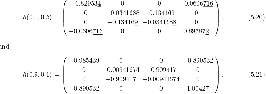
In order to compare with the results obtained in section 4 we give below the numerical values of the entries of the Hermitian Hamiltonianh(λ, κ) for fixed values of the couplings

h(0.1,0.5) =

    

−0.829534 0 0 ₋0.0606716 0 ₋0.0341688 ₋0.134169 0 0 ₋0.134169 ₋0.0341688 0 −0.0606716 0 0 0.897872

    

, (5.20)

and

h(0.9,0.1) =

    

−0.985439 0 0 ₋0.890532 0 ₋0.00941674 ₋0.909417 0 0 ₋0.909417 ₋0.00941674 0 −0.890532 0 0 1.00427

    

. (5.21)

We underlined the digits which differ from the exact values computed in (4.31) and (4.32) and note that the perturbative expressions for h(0.1,0.5) and h(0.9,0.1) agree extremely well with them, especially for smaller values ofκ, as is expected.

In order to see how fast this precision is reached in the perturbation theory we report in table 3 the relative error for the entryh11order by order up to 15

λ, κ_\O(κ) 2 4 6 8 10 12 14

[image:21.612.86.513.231.382.2]

0.9,0.1 5.7 10−4 4.6 10−5 4.7 10−6 5.3 10−7 6.4 10−8 8.2 10−9 1.1 10−9 0.1,0.5 2.5 10−2 6.3 10−3 2.1 10−3 7.5 10−4 2.9 10−4 1.6 10−4 4.7 10−5

Table 3: Relative error = —(perturbative value - exact value) / exact value— for h11 order by

order.

We observe that the convergence is fairly fast, which allows to extract useful information from the perturbation theory even at low order. We shall not be concerned here with more rigorous mathematical arguments regarding the summability and convergence in general.

5.2 The N = 2 case: perturbation theory in λ

around the exact solution forλ= 0 provided in section 4.1 and treat the nearest neighbour interaction term as perturbation. As announced already in section 3.2., we decompose

H(λ, κ) into

H(λ, κ) = ˜H0(κ) +λh˜1, where H˜0(κ) =−1

2(S

N

z +iκSxN), ˜h1=−1

2S

N

xx. (5.22)

We wish now once again to solve the equations (3.8) for the Dyson mapη, that is

H†(λ, κ) =ewH(λ, κ)e−w, (5.23)

where we have assumed thatη admits the exponential form

η =ew/2 with w=

∞

X

a=0

λawa(κ). (5.24)

At order λ0 equation (5.23) becomes simply

˜

H₀†(κ) =ew0(κ)_H˜

0(κ)e−w0(κ). (5.25)

The solution to this equation for allN was found in subsection 4.1 and corresponds to the Dyson map identified in equation (4.7). For N = 2 this means that

w0(κ) =−arctanh(κ)Sy2. (5.26)

Employing the once again the Backer-Campbell-Hausdorff identity to select_O(λ) terms in (5.23) we find the condition

˜

h1 =ew0(κ)h˜1e−w0(κ)+

∞

X

k=1

k

X

i=1

X

ai=1,

aj6=i=0

1

k![wa1(κ),[wa2(κ),· · · ,[wak(κ), H0(κ)]· · ·]] (5.27)

Notice that, because of the presence of the zeroth order term w0(κ), the equation (5.27)

involves a sum of infinitely many contributions, as would equations corresponding to higher orders in perturbation theory. Because of this, it would in general be difficult to solve (5.23) using perturbation theory inλ. However, forN = 2 we can solve up to high orders inλby exploiting the fact that η must have the structure identified in the previous section. This means that η is a matrix of the form (5.9) with

α(λ, κ) =

∞

X

a=0

λaya(κ), β(λ, κ) =

∞

X

a=0

λaza(κ). (5.28)

It is then possible to find the real functions ya(κ) and za(κ) which solve equation (5.23)

we will just report the first five orders,

y0(κ) = −arctanh(κ), (5.29)

z1(κ) =

y0(κ)

1₋κ2, (5.30)

y2(κ) = −

2(κ+ 2κ3+ 1₋κ2

y0(κ))

(1₋κ2₎3 , (5.31)

z3(κ) = −

2(κ+ 2κ3+ 1₋κ2₋2κ4

y0(κ))

(1₋κ2₎4 , (5.32)

y4(κ) =

2 κ 3₋5κ2_−32κ4_−8κ6

+ 3₋6κ2_−5κ4_{+ 8κ}6

y0(κ)

(1₋κ2₎6 , (5.33)

z5(κ) =

2 κ 3₋5κ2₋36κ4₋16κ6

+ 3₋6κ2₋9κ4+ 28κ6+ 8κ8

y0(κ)

(1₋κ2₎7 ,(5.34)

and y2a+1(κ) = z2a(κ) = 0 for all a = 0,1, . . . From these formulae, it is possible to find

an expression for the Hermitian Hamiltonian h(λ, κ) as a perturbative series in λ. As it should be, one finds the same structure (5.14) with

h11(λ, κ) =−

p

1₋κ2₊ κ2λ

1₋κ2 −

6₋2 +κ2+ 2√1₋κ2_λ2

(1₋κ2₎52

+ 4κ

4_λ3

(1₋κ2₎4

−

240₋44κ2₋57κ4+ 28κ6+ 8√1₋κ2 _{−5 + 3κ}2_{+ 8κ}4

λ4

(1₋κ2₎112

+_O(λ5), (5.35)

h22(λ, κ) =−

κ2_λ

1₋κ2 −

4κ4_λ3

(1₋κ2₎4 +O(λ

5_{), (5.36)}

h44(λ, κ) =

p

1₋κ2₊ κ2λ

1₋κ2 +

6₋2 +κ2+ 2√1₋κ2_λ2

(1₋κ2₎52

+ 4κ

4_λ3

(1₋κ2₎4

+

240₋44κ2_−57κ4_{+ 28κ}6_{+ 8}√_1−κ2 _{−5 + 3κ}2_{+ 8κ}4

λ4

(1₋κ2₎112

+_O(λ5), (5.37)

h14(λ, κ) =

−4 + 4κ2+ 3√1₋κ2_λ

(1₋κ2₎32

+

48₋10κ2₋2κ4+ 4κ6+√1₋κ2 _{2 +κ}2

−4 + 5κ2

λ3

(1₋κ2₎92

+_O(λ5). (5.38)

Notice that the same symmetries (5.19) are also found here. We also see once again that

relative error for the entryh11order by order up to 15, omitting the odd orders despite the

fact that they occur in theλ-perturbation theory

λ, κ_\O(λ) 2 4 6 8 10 12 14

[image:24.612.83.516.118.168.2]

0.9,0.1 3.4 10−3 2.3 10−5 1.9 10−6 1.8 10−7 1.9 10−8 2.0 10−9 2.2 10−10 0.1,0.5 1.1 10−3 6.3 10−5 4.9 10−6 3.6 10−7 3.1 10−8 2.8 10−9 2.6 10−10

Table 4: Relative error = —(perturbative value - exact value) / exact value— for h11 order by

order.

We note that the perturbation theory converges extremely fast, even for large values of λ, for which one would not expect such a behaviour. This can be explained as follows: In the domain of unbroken _PT-symmetry UPT the allowed values for κ become very small asλ

increases. As we note from the expressions (5.35)-(5.38) the order of κ increases with the order ofλterm by term.

5.3 The N = 3 case

We will now carry out an analogous perturbative study in κ for the three sites case. We keep the choice of periodic boundary condition, even though for sites more than two this means some loss of generality. Proceeding as before, we will try to obtain the matrix q

perturbatively, by solving the consistency conditions (3.18)-(3.20). Now we have to solve the problem for 8_×8-matrices. We commence by computing the kernel of h0

B1 =I, B2 =Szz3 −λSyyz3 , B3 =λSyy3 −(1−λ2)Syyz3 −Sxxz3 , B4 =Sxy3 −Syx3 ,

B5 =Szzz3 , B6 =Sxyz3 −Syxz3 , B7 =λSxx3 +Sz3 =−2h0(λ), B8 =Sxx3 +Syy3 +λSyyz3 ,

in addition to this eight matrices, there are another four, due to the fact that two of the eigenvalues ofh0(λ) are degenerate. Hence the dimension of the kernel is 12,

B9 = Sz3−λ(Syy3 +Szz3 −σ y

1σ

y

3−σz1σz3−σx1σx3), B10=σy2σ

y

3 +σz2σz3+σx2σx3, (5.39)

B11 = Szz3 +λSxxz3 −λ(σ1z+σz3+σx1σz2σx3+σy1σz2σy3), B12=σ3z−σx1σx2σz3−σy1σ

y

2σz3,

with [Bi, h0(λ)] = 0 for i= 1, . . . ,12. Similarly as in the case N = 2 we find that all of

these matrices are parity invariant

PBiP =Bi, ∀ i= 1, . . . ,8, (5.40)

which from equations (3.26) means that no linear combination of the matrices Bi can be

added toq2k−1that would be compatible with the constraints (3.24). Therefore, with such

constraints, there is a unique solution to (3.18) which has the form,

q1(λ) =−Sy3−λ(Syz3 +Szy3 ) + 2λ2(Syyy3 −Szzy3 ). (5.41)

As we can see, the two first terms inq1(λ) are a direct generalization of the result for two

S3

xxy (fork= 1, equation (5.1) tells us though that the coefficient ofSxxy3 is zero. This will

change for higher orders in perturbation theory). We can therefore write,

q= ˆα(λ, κ)S_y3+ ˆβ(λ, κ)(S3_yz+S_zy3 ) + ˆγ(λ, κ)S_yyy3 + ˆδ(λ, κ)S_xxy3 + ˆǫ(λ, κ)S_zzy3 , (5.42)

where

ˆ

α(λ, κ) = X∞

k=1ˆa2k−1(λ)κ

2k−1_{, βˆ(λ, κ) =}X∞

k=1

ˆ

b2k−1(λ)κ2k−1, (5.43)

ˆ

γ(λ, κ) = X∞

k=1ˆs2k−1(λ)κ

2k−1_{, ˆδ(λ, κ) =}X∞

k=1

ˆ

d2k−1(λ)κ2k−1, (5.44)

ˆǫ(λ, κ) = X∞

k=1ˆe2k−1(λ)κ

2k−1_{. (5.45)}

Computing coefficients up to order κ7 _{we find the results in tables 5-7.}

−λ0 −λ2 −λ4 −λ6 −λ8 −λ10 −λ12

ˆ

a1(λ) 1 0 0 0 0 0 0

ˆ

a3(λ) 1 3

8

3 16 0 0 0 0

ˆ

a5(λ) 1₅ 122₁₅ 144 5024₁₅ 3072₅ 0 0 ˆ

a7(λ) 1₇ 576₃₅ 9616₁₅ 432832₁₀₅ 1755136₁₀₅ 2720768₁₀₅ 196608₇ ˆ

d1(λ) 0 0 0 0 0 0 0

ˆ

d3(λ) 0 0 2₃4 0 0 0 0

ˆ

d5(λ) 0 2 3 496 15 1184 15 210

5 0 0

ˆ

[image:25.612.125.513.124.245.2]

d7(λ) 0 2₁₅5 4432₃₅ 86848₁₀₅ 65024₁₅ 754688₁₀₅ 216₇

Table 5: The coefficients ˆa2k+1(λ) and ˆd2k+1(λ) fork <4.

−λ −λ3 −λ5 −λ7 −λ9 −λ11 −λ13

ˆ_{b1(λ) 1 0 0 0 0 0 0,}

ˆ_b3(λ) 4 3

28 3

26

3 0 0 0 0

ˆ_b5(λ) 23 15 664 15 1568 5 3328 5 212

5 0 0,

[image:25.612.141.463.180.241.2]

ˆ_b7(λ) 176 105 4344 35 13536 7 52416 5 1104384 35 311296 7 218 7

Table 6: The coefficients ˆb2k+1(λ) fork <4.

−λ2 −λ4 −λ6 −λ8 −λ10 −λ12 −λ14

ˆ

s1(λ) -2 0 0 0 0 0 0

ˆ

s3(λ) -4 -8 −237 0 0 0 0

ˆ

s5(λ) −285 − 112 5 − 2592 5 − 4608 5 − 213

5 0 0

ˆ

s7(λ) −232 35 288 35 − 91008 35 − 452224 35 − 356352 7 − 491520 7 219 7 ˆ

e1(λ) 2 0 0 0 0 0 0

ˆ

e3(λ) 20₃ 56₃ 2₃7 0 0 0 0

ˆ

e5(λ) 196 15 400 3 3872 5 6656 5 213

5 0 0

ˆ

[image:25.612.139.458.565.700.2]

e7(λ) 440₂₁ 53152₁₀₅ 206336₃₅ 75904₃ 69632 622592₇ 219₇

It is now possible to use these perturbative results to compute h(λ, κ) for particular values ofλand κ. We find that the structure of the Hermitian counterpart of the original Hamiltonian is:

h(λ, κ) = µ3_xx(λ, κ)S_xx3 +µ3_yy(λ, κ)S_yy3 +µ3_zz(λ, κ)S_zz3 +µ3_z(λ, κ)S_z3

+µ3_xxz(λ, κ)S_xxz3 +µ3_yyz(λ, κ)S_yyz3 +µ3_zzz(λ, κ)S_zzz3 , (5.46)

which resembles the result for two sites, but includes few extra terms that couple all three sites. The functions µ3_xx, . . . , µ3_zzz are all real functions of the couplings. As for N = 2, the Hamiltonian above is _PT-symmetric, which follows from the fact that all matrices involved are invariant under the adjoint action of the operator _PT (see equation (4.5)). As for N = 2 also, these are the only matrices that are both _PT symmetric and real (notice that, from the definition (4.1) for N = 3, it holds that S3

xxz = Szxx3 = S3xzx and S_yyz3 =S3_zyy =S_yzy3 ).

5.4 The N = 4 case

It is interesting to investigate how the perturbative results generalize as we increase the number of sites. The N = 4 case is especially interesting as it is the simplest example for which we may see non local interaction terms in the Hermitian Hamiltonian. There is again only one solution forq1(λ) which is compatible with the conditions (3.26), that is

q1(λ) = −Sy4−λ(Syz4 +Szy4 )−

6λ3(S4

yuz−Syz4 −Szy4 )

40λ2₋9

+ 1

40λ2₋9

(9₋32λ2)λ2(S_yzz4 +S_zzy4 )₋32λ4S_zyz4 ₋2λ2(3₋16λ2)S_yyy4

−3λ2(S_xxy4 ₋2S_xyx4 +S_yxx4 ) + 2λ3(S_xxyz4 ₋5S_xyxz4 +S_xxzy4 ) + 2λ3(9S_yzzz4 ₋7S_yyyz4 ) + 64λ5(S4_yyyz−S_zzzy4 )

. (5.47)

In many ways, this is a simple generalization of the results of two and three sites. The matrices that enter the expression are to a large extent the same we find for less sites, but we have now extra contributions involving Pauli matrices sitting at all four sites of the chain, which was to be expected. There are however two major changes

• the dependence on λof the coefficients is not polynomial anymore,

• the first occurrence of non-local interactions appears through the matrixS4

yuz.

As for lower values of N, it is not difficult to argue that the matrices (4.1) entering the linear combination (5.47) are the only ones that are compatible with (3.24). Hence, as expected, the same structure extends to higher orders in perturbation theory, although expressions become extremely involved. The table below gives q3(λ) as a sum of terms