Comparison of structured- and unstructured-grid, compressible and incompressible methods using the vortex pairing problem

.

Comparison of structured- and unstructured-grid, compressible and

incompressible methods using the vortex pairing problem.

Panagiotis Tsoutsanis, Ioannis W. Kokkinakis, L´aszl´o K¨on¨ozsy, Dimitris Drikakis

Fluid Mechanics and Computational Science, Cranfield University, Cranfield, MK43 0AL, United Kingdom

Robin J.R. Williams, David L. Youngs

AWE, Aldermaston, Reading RG7 4PR, United Kingdom

Corresponding author: Prof Dimitris Drikakis, Fluid Mechanics and Computational Science Centre,

Abstract

The accuracy, robustness, dissipation characteristics and efficiency of several structured and unstructured grid methods

are investigated with reference to the low Mach double vortex pairing flow problem. The aim of the study is to shed

light into the numerical advantages and disadvantages of different numerical discretizations, principally designed

for shock-capturing, in low Mach vortical flows. The methods include structured and unstructured finite volume

and Lagrange-Remap methods, with accuracy ranging from 2nd _{to 9}th_{-order, with and without applying low-Mach}

corrections. Comparison of the schemes is presented for the vortex evolution, momentum thickness, as well as for

their numerical dissipation versus the viscous and total dissipation. The study shows that the momentum thickness

and large scale features of a basic vortical structure are well resolved even at the lowest grid resolution of 32×

32 provided that the numerical schemes are of a high-order of accuracy or the numerical framework is sufficiently

non-dissipative. The implementation of the finite volume methods in unstructured triangular meshes provides the

best results even without low Mach number corrections provided that a higher-order advective discretization for the

advective fluxes is employed. The compressible Lagrange-Remap framework is computationally the fastest one,

although the numerical error for the momentum thickness does not reduce as fast as for other numerical schemes and

computational frameworks, e.g. , when higher-order schemes are utilized. It is also shown that the low-Mach number

correction has a lesser effect on the results as the order of the spatial accuracy increases.

1. Introduction

The presence of a wide-range of spatial and temporal scales in complex flows featuring vorticity dynamics

pro-hibits the use of direct numerical simulations to resolve all of the scales within a flow, even with today’s computing

power, and it is expected that it will remain the case in the foreseeable future. Therefore, in many practical

applica-tions the simulaapplica-tions still remain under-resolved, such that the large scales are resolved and the smallest scales are

modeled.

It is well known that high-order schemes are superior to low-order ones both in terms of accuracy and

computa-tional efficiency. However, high-order schemes usually lack the robustness of their low-order counterparts.

Further-more, it is not yet well understood how different unstructured and structured-grid based computational frameworks

and numerical discretisation schemes influence the accuracy (and efficiency) of simulations in vortical flows. The

notconcern an assessment of the accuracy of numerical methods in turbulent flows, the methods employed here are

widely used in implicit large eddy simulations (ILES) [1–4], which rely on the non-linear numerical dissipation of

high-resolution schemes to locally and dynamically produce similar effects achieved by explicit subgrid models used

in classical LES. Since the accuracy of numerical schemes used in ILES is sensitive to the critical balance of the

dissipation and dispersion contributions to the numerical solution [5–9], which strongly depend on the design details

of each high-resolution non-oscillatory finite volume method, it is of paramount importance to understand the

perfor-mance of high-order schemes in prototypical vortical flows, especially when using under-resolved grid arrangements.

Therefore, the numerical accuracy issues for the double vortex pairing (DVP) problem are also pertinent to more

complex flows.

Four different numerical frameworks are used in this study. These are an incompressible structured-grid finite

vol-ume, a compressible structured-grid finite volvol-ume, a compressible unstructured-grid finite volvol-ume, and a compressible

Lagrange-Remap framework. Determining which of these frameworks is “the best” isnotthe scope of the study, as it

is appreciated that each of these frameworks may exhibit different behavior depending on the types of flow problems

encountered. On the other hand, it is essential to understand the underlying characteristics of each of these numerical

frameworks when used in conjunction with high-resolution/high-order schemes at coarse grid resolutions and for low

Mach number flows such as the basic double vortex pairing problem.

The test problem is related to the experimental work carried out by Winant and Browand [10], who investigated

the vortex formation in a shear layer and the subsequent double vortex interaction and pairing process into a single

vortex. A mixing layer is formed by bringing two streams of water, moving at different velocities, together in a

lucite-walled channel. In the experiments conducted [10] it was observed that unstable waves grow downstream and the

fluid subsequently rolls up into discrete two-dimensional vortical structures. These turbulent-like vortices interact by

rolling around each other, ultimately forming a single vortical structure with approximately twice the spacing of the

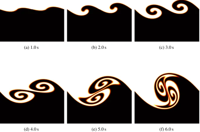
former vortices as illustrated in Figure1. This pairing process is observed to occur repeatedly, controlling the growth

of the mixing layer.

The flow conditions (stream velocities, length-scales, Reynolds number etc.) investigated in the numerical

simula-tions are taken from the aforementioned experiment with the aim of calculating the evolution of some of the observed

large-scale structures. Simulation of vortical flows requires modeling as wide a range of structure sizes as possible

(i.e. maximizing the achievable dynamic range). Hence, one method of testing the suitability of the numerics is to ask

the question: “What is the lowest resolution that can be used to model a basic vortical structure?”

The objective is to demonstrate the capability of compressible and incompressible high-resolution methods to

(a) 1.0 s (b) 2.0 s (c) 3.0 s

(d) 4.0 s (e) 5.0 s (f) 6.0 s

Figure 1: Time evolution of the double vortex pairing process on a 2562grid cell resolution using the WENO 9thorder scheme in the compressible structured-grid framework; passive scalar contours (c=0.25, c=0.5, c=0.75).

in highly compressible flows, small scale vortical structures are usually low Mach number features. Hence the test

problem is of relevance to a range of compressible and incompressible flows. The numerical method survey

con-ducted consists of a structured-grid finite-volume compressible solver using high-order reconstruction methods with

1D swept directional stencils; a compressible unstructured-grid solver, also using high order reconstruction methods,

but allowing for multidimensional stencils; a compressible Lagrange-remap solver (LR); and an incompressible finite

volume structured-grid solver in order to include a reference high-resolution incompressible solution for the present

low speed problem. Viscosity is included in the test problem and the highest resolution simulations (2562_{) fully}

resolves the velocity field.

The paper is organized as follows. First, the initial and boundary conditions of the double vortex pairing are

described in§2. Then, in§3, a description of the numerical methods and frameworks employed in this study are

presented, followed by a presentation in §4 of all the statistical quantities used in assessing the accuracy of the

schemes. The results obtained by the various schemes and frameworks are categorized in terms of vortex evolution,

momentum thickness, (numerical) kinetic energy dissipation and computational efficiency in subsections§5.1,5.2,

2. Double Vortex Problem Description

2.1. Initial and Boundary Conditions

The initial conditions described in [10] consist of two co-flowing velocities,u1=4.06 cm/s (lower stream) and

u2=1.44 cm/s (upper stream). The mixing layer comprises of a single component, single phase fluid. The calculation

is performed in a frame of reference moving with the mean stream velocity,U=2.75 cm/s, and focuses on the evolution

of the large scale vortex from the two original smaller vortices. The final structure has a wavelength ofL≈6 cm, which

is the length of the edges of the computational box used to contain the double vortex evolution and subsequent merger

(Fig.1).

The two streams have a velocity difference of∆U=2.62 cm/s and same physical properties such as density and

viscosity. The computations performed maintain the velocity difference∆U=2.62 cm/s but assign equal and opposing

free-stream velocities to the two layers similar to other numerical double vortex pairing investigations [11]. Thus the

free-stream properties for velocity areULower

∞ = ∆U/2=1.31 cm/s andU

U pper

∞ =−U∞Lower, densityρ∞=1 gr/cm3 and kinematic viscosityν∞=0.01 cm2_{/s. The Mach number based on the relative velocity of the two streams (∆U) is equal}

to 0.2, or otherwise based on the free-stream velocity (the so-called convective Mach number) equal to 0.1. In either

case the free-stream speed of sound is given byα∞=

p_γ

P∞/ρ∞. Finally, the adiabatic indexγis equal to 5/3 for an

ideal monatomic gas and the free-stream pressure isP∞=10.3 N/m2and assumed constant in the domain. Note that

the Mach number can also be lowered by simply increasingP∞.

The unperturbed streamwise velocity profile is given by equation:

u=−1

2∆Utanh

y

2θ0 !

(1)

whereθ0is the initial momentum thickness equal to 0.03 cm.

The Reynolds number based on∆U,LandνisRe =(∆U)L/ν =1600. A stream function (ψ) is used to add a

divergence-free initial perturbation to both velocity components (u0_,v0_{). The fluctuations are calculated as:}

u0=−∂ψ

∂y, v

0₌ ∂ψ

∂x (2)

The stream functionψis the sum of two Kelvin-Helmholtz instability eigenmodes given by [12]:

ψ=A1(y)ν1

k1cos (k1x) exp (−k1|y|)+A2(y)

ν2

with the two corresponding wavenumbers,k1andk2, set equal to:

k1=

2π

L , k2=

4π

L (4)

and

Ai=

1−exph−2ki _L

2− |y|

i

1−exp (−kiL)

(5)

The two velocity amplitudes areν1=0.025∆Uandν2=0.05∆U. Similar to previous numerical studies [11], the

boundary conditions are periodic in the x-direction (streamwise) and reflective (∂v/∂y =0) in the y-direction. The

reflective condition in the y-direction is required to avoid viscouss dissipation at the boundaries.

3. Description of methods

3.1. Compressible methods

The 2D viscous compressible Navier-Stokes with heat conduction are considered in the following form:

∂ ∂tU+

∂

∂x(Fu−Gu)+

∂

∂y(Fv−Gv)=0 (6)

whereUis the vector of the conserved variables,Fu,Gu, andFv,Gv are the convective and viscous flux vectors in

x,yCartesian coordinates directions respectively, given by:

U=                                         ρ ρu ρv E ρϕ                                        

, Fu=

                                        ρu

ρu2_+p

ρuv

u(E+p)

ρuϕ                                        

, Fv =

                                        ρv ρvu

ρv2+p

v(E+p)

ρvϕ                                         ,

Gu=

                                        0 τxx τxy θx 0                                        

, Gv=

whereρis the density,uandvare the velocity components in thexandydirections respectively,prepresents static

pressure,E = p/(γ−1)+0.5ρ(u2+v2) is the total energy per unit volume,ϕis a passive scalar,γis the ratio of

specific heats,τi jthe stresses tensor, andθis defined by the following relations:

θx=uτxx+vτxy+

µγ

Pr(γ−1) ∂T

∂x

θy=uτyx+vτyy+

µγ

Pr(γ−1) ∂T

∂y

The ideal gas law is used withγ=5/3,T =p/ρis the temperature,Pris the Prandtl number andµis the dynamic

viscosity; the initial conditions and fluid parameters were previously defined in§2.1.

The spatial domain is discretized by conforming elements. Its cell elementiof volumeVi(area for 2D), can be

of triangular or quadrilateral shape as shown in Figure3. Integrating equation (6) over a mesh element, leads to the

following semi-discrete finite-volume formulation:

d dtUi+

1

Vi I

∂Vi

Fc_n−Fv_ndA=_{0 (7)}

whereAis the length of the corresponding side, andFc_n−Fv_n are the projections of the convective and viscous flux vectors normal to the sides given by:

Fc_n=                               

ρVn

ρuVn+nxp

ρvVn+nyp

Vn(E+p)                               

, Fv_n=                                0

nxτxx+nyτxy

nxτyx+nyτyy

nxθx+nyθy                               

Ui(t) is the conserved vector at time levelt, and Vnis the velocity normal to the sideAdefined by Vn =nxu+nyv.

Assuming that the element consists ofLsides and denoting bynjthe outward unit vector for sideAj, then the integral

over the element boundary∂Visplits into the sum of integrals over each side resulting in the following expression:

d

dtUi=Ri (8)

with

Ri=−1 Vi

L X

j=1 Z

Aj

Fc_n,jdA+ 1 Vi

L X

j=1 Z

Aj

Figure 2: Structured solver reconstruction stencils (1D-split) for a 5thorder scheme.

A passive scalar field (ϕ) is used to visualize the formation process of the vortices and merger. The passive scalar

is advected according to the resolved viscous velocity field and is therefore given by:

dρϕ dt +

1

Vi I

∂Vi

VnρϕdA=0 (9)

In the case of the incompressible structured-grid framework, the solution is advanced in time using a dual-time

stepping method with inner pseudo-time steps and the passive scalar is therefore given by:

∂ϕ ∂τ =−

∂ϕ

∂t −(u· ∇)ϕ (10)

3.1.1. Compressible structured-grid framework

The structured-grid code solves the full Navier-Stokes equations using a finite volume Godunov-type [13,14]

method. The intercell numerical fluxes are computed based on the solution to the Riemann problem using the

re-constructed variables at the left and right (or upper and lower) cell interfaces. The reconstruction stencil is a

one-dimensional swept directional stencil, as illustrated in Figure2.

The Riemann problem is solved using the Harten, Lax, van Leer, and (the missing) “Contact” (HLLC) approximate

Riemann solver [15]. The reconstructed values utilized in the HLLC Riemann solver are obtained primarily by two

different limiter approaches, the Monotone Upstream-centered Schemes for Conservation Laws (MUSCL) [16] and

the Weighted-Essentially-Non-Oscillatory (WENO) reconstruction methods [17]. For each reconstruction technique

a variety of differing orders of accuracy are examined, all of odd number. MUSCL is employed using 3rdand 5thorder

of accuracy schemes [18,19] (henceforth labeled in the figures as M3 and M5, respectively), whereas WENO uses the

5th_{and 9}th_{order of accuracy schemes [20,21] in conjunction with the relative smoothness limiter of [22] (henceforth}

labeled as W5 and W9, respectively), which are extensions of the original WENO scheme [17].

All the reconstruction techniques used in this paper have been further augmented with a low-Mach limiting scheme

[23], which involves an additional stage in the reconstruction process for the velocity vector. This low-Mach number

the validity of Godunov type method to at least Mach ≈10−4 via a progressive central differencing of the velocity

components. The viscous part of the equations is solved using a second order central difference scheme. Finally,

the solution is advanced in time using a three-stage total variation diminishing (TVD) Runge-Kutta (RK) method

[14,15,24].

3.1.2. Compressible unstructured-grid framework

The numerical approach of [25,26] is adopted in the present study which is suitable for unstructured meshes with

various types of element shapes in 2D and 3D, where it has been previously used successfully for laminar, transitional

and turbulent flows [27,28]. A Gaussian numerical quadrature of appropriate order for the order of the polynomial

used is implemented for the approximation of the integral expressions of the fluxes.

The calculation of the numerical convective and viscous fluxes requires the knowledge of the pointwise values

of the conserved vector as well as the velocity and temperature gradients at each Gaussian integration point. These

pointwise values are approximated through an interpolation (reconstruction) procedure of a desired order of accuracy

utilizing the cell averages. The latter requires a recursive stencil construction process where the direct side neighbor

elements are added until a target number M of stencil elements has been reached. For MUSCL types of schemes

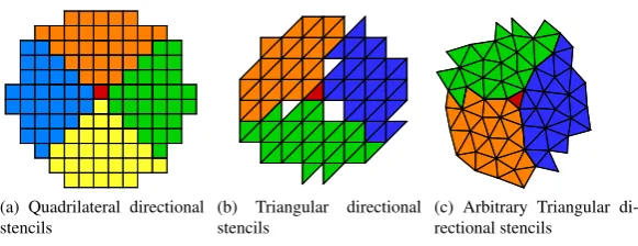
only one central stencil is used, however for WENO schemes, in addition to the central stencil, several additional

directional stencils are also used as shown in Figure3.

The reconstruction is carried out in a transformed system of co-ordinates in order to minimize scaling effects that

appear in stencils consisting of elements of different sizes, as well as to improve the condition number of the system

of equations [25,26]. For computing the degrees of freedom, a minimum ofK cells are needed in the stencil in

addition to the target cell. Using the minimum possible number of cells in the stencil (M ≡ K) has been found to

produce ill-conditioned systems [26,29–31], hence the choice to useM=2Kimproves the robustness of the method.

This is especially worthwhile since no substantial performance penalty is incurred as a result of this improvement

[26,31,32]. The resulting least-squares system is solved by a QR decomposition and the reconstruction polynomial

is computed.

In the present study two types of schemes are employed for the convective part, a MUSCL type of scheme using

the TVD-type slope limiter of Barth and Jespersen [33] and the WENO implementation of [25,26] carried out in

characteristic variables, both of them satisfying thek-exactness criteria. For the viscous part a linear reconstruction

polynomial of the same order for the velocity and temperature field is constructed using the same central stencil as

for the conserved vector. The discontinuous states of the convective fluxes are approximated by the HLLC Riemann

solver of Toro [15], and the central averaging approach is used for the discontinuous viscous flux. The solution is

(a) Quadrilateral directional stencils

(b) Triangular directional stencils

(c) Arbitrary Triangular di-rectional stencils

Figure 3: Unstructured-grid solver multidimensional stencils for a 5th_{order scheme using different types of elements;}

considered element in red color.

grids for complex geometries can benefit when combined with variational optimization techniques [34], as well as the

use of very high order methods such as the ones proposed in [35].

3.2. Compressible Lagrange-Remap framework

The numerical approach of [2] is used in the present study. In particular, a staggered grid arrangement is employed

with densityρ, internal energyeand pressurepdefined at cell centers, and velocity components,uandv, defined at

cell vertices. The viscous compressible Navier-Stokes equations are solved and the calculation for each time step

is divided into two phases. The first phase can be considered as a Lagrangian and the second phase which is the

advection one, transports mass, internal energy and momentum across cell boundaries. For low Mach number the

Lagrangian phase is divided into several steps, hence the overall time step is thereby less constrained by the sound

speed. In the advection phase, the monotonic method of Van Leer [36,37] is used for all fluid variables. It must also

be noted that all the flow variables for a given cell at the end of the advection phase lie within the range of values for

the cell and its neighbors at the end of the Lagrangian phase. The Lagrange phase is non-dissipative in the absence

of shocks. Artificial viscosity,q, is used to provide dissipation due to shocks. For the present near-incompressible

test problem, this dissipation (q∇u) is negligible. As a result the method does not become dissipative at low Mach

number. It must be stressed that in order to have the same initial conditions as the other cell-centered frameworks due

the staggered grid arrangement the meshes employed are 33×33, 65×65 and 257×257 points, which are henceforth

labelled as 322_{, 64}2_{and 256}2_.

3.3. Incompressible structured-grid framework

An incompressible method was also employed in order to compare the low-speed compressible simulations with

effect of the gravity field are written as:

∇ ·u=0, (11)

∂u

∂t +∇ ·(u⊗u)=−

1

ρ∇p+υ∇2u (12)

wheretis the physical time, uis the velocity field, p is the hydrodynamic pressure, ρis the fluid density, andυ

is the kinematic viscosity of the fluid. For the solution of the incompressible equations a method that combines

the fractional step (FS) pressure-projection (PP) [38–40] and artificial compressibility method (AC method) [41] has

been employed. Details for the unified FSAC-PP method are given by K¨on¨ozsy and Drikakis [42]. The method has

shown superior accuracy and efficiency characteristics compared to the FS-PP and AC approaches for a range of test

problems [42,43]. The characteristics-based (CB) scheme [44–46] is employed for discretizing the convective fluxes.

The method falls into the category of pseudo-time splitting FSAC approaches, including a PP step at each pseudo-time

step of the dual-time stepping procedure for accelerating the solution towards the incompressibility (divergence-free)

constraint. After performing the pseudo-time advancement, the pressure field is computed to update the CB velocity

components at each pseudo-time step. By taking the divergence of the semi-discrete equation, similarly to the FS-PP

method [39,47], the cell-centered pressure values are obtained by solving an elliptical pressure-Poisson equation at

each pseudo-time step. The numerical solution for the velocity field provides an approximately divergence-free vector

field at each pseudo-time step.

The CB scheme has been implemented in conjunction with an upwind 3rd_{order extrapolation [44–46] (henceforth}

labeled as U3), as well as with the MUSCL 5th_{(M5), WENO 5}th _{(W5) and WENO 9}th _{(W9) order schemes. The}

Gauss-Seidel-type Successive-Over-Relaxation (S.O.R) iteration method [48,49] is used for solving the discretized

elliptical pressure-Poisson equation. The viscous flux terms are approximated by second-order central schemes. The

temporal accuracy of pseudo-time stepping procedure can be advanced by applying a Runge-Kutta time integration

scheme [24,45].

4. Double Vortex Statistics

We first clarify that the double vortex problem is solved in 2D (defined here as the xy-plane). Thus the 3rd

(z-direction) spatial component is omitted throughout.

Various properties of the double vortex formation and merger are investigated. A passive scalar field (ϕ) is used in

be used for a qualitative comparison between the various schemes and numerical frameworks. In order to conduct

quantitative comparisons, the momentum thickness and numerical dissipation are additionally obtained.

The momentum thickness (θ) is used in order to investigate the growth rate and is calculated as:

θ= ∞

Z

y=−∞

_u

1−u(y) u(y)−u2

(u1−u2)2 dy (13)

whereu1andu2 are the lower and upper stream velocities. By replacingu1 = ∆U/2 = −u2, equation (13) can be

re-written as:

θ= ∞

Z

y=−∞

      

1 4−

" u(y)

∆U #2

     

dy (14)

If the velocity is non-dimensionalized by∆U(u∞) it is possible to compute the above integral over a domain of

sizeL×Lnumerically as:

θ=

L X

y=0 "

1 4 −u¯(y)

2 #

∆y (15)

where∆yis the cell height, and ¯u(y)=PL_x=0u(x,_y)∆_x/_{Lis the average velocity along the streamwise direction.}

As previously mentioned in the introduction, the numerical methods considered herein are implemented within

the framework of ILES. If the flow has not been sufficiently resolved, part of the dissipation of kinetic energy is

attributed to the implicit numerical dissipation. In order to assess the performance of the various numerical methods,

we quantify and compare the numerical dissipation (DN) produced by each method. The total loss of kinetic energy

at any cell occurs due to the inviscid advection and viscous diffusion. Since viscous diffusion is typically treated by a

central order approximation, it does not produce any numerical dissipation. On the contrary, the non-linear advection

terms are well known to dissipate kinetic energy when using upwind-type methods. Though there is no known way

of quantifying the amount of numerical dissipation at any given cell separately, it is completely plausible to quantify

the total kinetic energy loss or dissipation of a closed (isolated) system. The double vortex problem considered here

is such a closed system since the boundary conditions do not allow for any kind of transfer, be it mass, momentum or

energy, in or out of the domain.

The systems total kinetic energy loss rate (DKE) due to viscous and numerical dissipation can be evaluated at any

time step as follows:

DKE =−∂

∂t Ly

Z

y=0 Lx

Z

x=0

1 2ρ

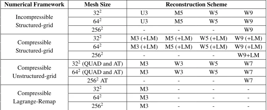
Numerical Framework Mesh Size Reconstruction Scheme

Incompressible Structured-grid

322 U3 M5 W5 W9

642 U3 M5 W5 W9

2562 _{- - - W9}

Compressible Structured-grid

322 _{M3 (+LM) M5 (+LM) W5 (+LM) W9 (+LM)}

642 M3 (+LM) M5 (+LM) W5 (+LM) W9 (+LM)

2562 - - - W9+LM

Compressible Unstructured-grid

322_{(QUAD and AT) M3 W3 W5 W7}

642_{(QUAD and AT) M3 W3 W5 W7}

2562_{AT - - - W7}

Compressible Lagrange-Remap

322 M3 - -

-642 _{M3 - -}

-2562 _{M3 - -}

-Table 1: Numerical schemes used and simulations performed. The schemes are labeled as U (upwind); M (MUSCL); W (WENO); LM (low-Mach); QUAD (Quadrilateral elements); AT (Arbitrary Triangular elements).

The total viscous dissipation (DV) is given by:

DV = Ly

Z

y=0 Lx

Z

x=0

µ

      

∂u

∂y+

∂v

∂x !2

+2

      

∂u

∂x !2

+ ∂_∂v

y !2

     

−2

3 ∂u

∂x+

∂v

∂y !2

     

dxdy (17)

By having determined the viscous dissipation (DV) it is now possible to obtain an estimate of the total numerical

dissipation:

DN =DKE−DV (18)

It is noted that the above is strictly true only for an incompressible flow. For the weakly compressible case,

acoustic modes are present which exchange internal and kinetic energy. Thus this approach of estimating the numerical

dissipation (DN) includes a superimposed oscillation on the true value.

5. Results

The computational results of all the numerical frameworks are presented in this section. The schemes are assessed

in terms of the vortex evolution pattern (§5.1), momentum thickness (§5.2), numerical dissipation (§5.3) and

compu-tational efficiency (§5.4). Table1provides a complete list summarizing all the numerical simulations conducted.

5.1. Vortex Evolution

The pattern of the vortex evolution, whereby the growth of unstable waves occurs as a result of the roll up of

the numerical schemes and frameworks encountered in the present study. The main objective is to assess the

character-istics of each numerical framework in under-resolved grid arrangements where the impact of the numerical schemes

on the vortex formation and structure (flow features resolved) is discussed. To this end, a “reference” simulation

obtained by each framework was required in order to ensure that all the methods converge to the same vortex pattern.

A very high grid resolution of 256×256 cells was chosen as the reference resolution for all simulations across the

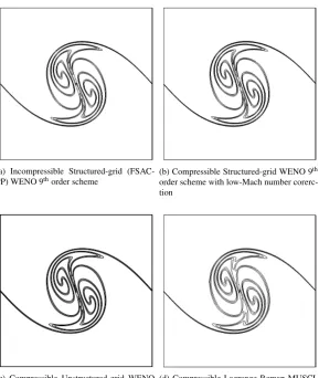
numerical frameworks employed, for which all methods should achieve identical results. As can be seen in Figure4,

where iso-lines of the passive scalar are plotted for values of 0.25, 0.5 and 0.75, all the schemes provide a similar

vortex structure att =6.0 s. This is particularly encouraging since it can be regarded as an indication that the flow

physics, at this resolution, is not greatly influenced anymore by the numerical schemes employed. Hence, the correct

flow pattern (defined as the vortex pattern at the finest resolution) can be presumed to have been captured.

In under-resolved grid arrangements this no longer holds and as a result the different numerical frameworks

re-solve substantially different vortex structures. As both compressible and incompressible numerical frameworks are

employed in the incompressible regime, it is essential to guarantee that the results obtained from the compressible

framework are Mach number converged. In other words, it is necessary to ensure that even when performing the

simulations at a very low Mach number of 0.02 with a compressible solver, the same vortex pattern is generated as at

0.2, less some deviations due to small compressibility effects. Moreover, it is critical to investigate the performance

of the schemes in this low-Mach number regime. For this purpose an initial qualitative comparison between all the

numerical frameworks is undertaken and the performance of each numerical framework is analyzed with regards to

the resolved final vortex structure.

In order to assess the effects of low-Mach number dissipation, we have performed incompressible simulations. For

the 32×32 grid (Figure5), increasing the nominal spatial order of accuracy from 3rd_{to 9}th_{order only slightly improves}

the results. In actuality, increasing the nominal accuracy does not result in a higher-order discretization on the coarse

grid because the majority of the discretisation stencils, particularly in the case of WENO schemes, encompass the

“discontinuity” of the mixing layer, thus the numerical scheme is forced (by design) to reduce its accuracy. As the

grid resolution further increases to 64×64 grid (Figure6), the effects of the accuracy become more evident, as more

detailed flow features inside the merged vortex region become visible.

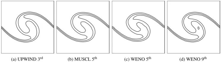
For the compressible structured-grid framework on the 32×32 grid (Figure 7), the results are sensitive to the

numerical scheme employed. Specifically, the angle of the vortex for the MUSCL 3rdis different than the one obtained

by the MUSCL 5th, WENO 5thand WENO 9th. The compressible structured-grid simulations compare well with the

incompressible results on the 32×32 grid, however, the vortex is more stretched in the WENO 5th _{and 9}th _order

(a) Incompressible Structured-grid (FSAC-PP) WENO 9th_{order scheme}

(b) Compressible Structured-grid WENO 9th

order scheme with low-Mach number corerc-tion

(c) Compressible Unstructured-grid WENO 7thorder scheme (Multi-dimensional stencils, Triangular elements)

(d) Compressible Lagrange-Remap MUSCL 3rdorder scheme

Figure 4: Overview of the final vortex structure obtained by all examined numerical frameworks for the reference 2562grid resolution at timet=6.0 s; passive scalar contours (c=0.25, c=0.5, c=0.75).

inside the vortex, which rise in number and detail as the order of accuracy increases (Figure8(d)).

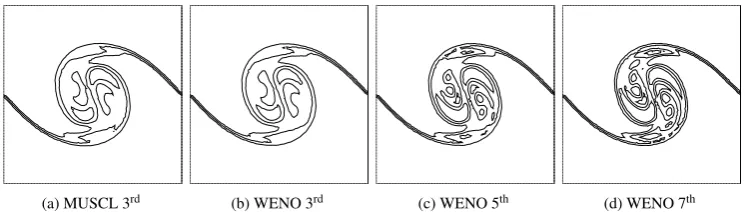
For the compressible unstructured-grid framework on the 32×32 grid the results are more sensitive to the numerical

scheme employed. For the 32×32 quadrilateral (QUAD) grid a 3rdorder scheme is not capable of resolving the two

initial vortices that merge into one single vortex (see Figure9). On the contrary, the high-order schemes (WENO 7th

in particular) are able to capture the correct vortex pattern.

A comparison between quadrilateral (QUAD) and arbitrary triangular (AT) meshes is presented in Figures10

and11for simulations on the 64×64 grid. The triangular meshes give a greater number of resolved features than

those seen by their quadrilateral counterparts. Furthermore, the compressible unstructured-grid framework is more

sensitive to the effects of the spatial order of accuracy and the type of grid used than the corresponding

stencils of the triangular grids[25,26].

The results for the final resolved vortex structure obtained from the compressible Lagrange-Remap framework

are presented in Figure12. The solution on the 32×32 grid (Figure12(a)) has the most accurately formed structure

than any of the other numerical frameworks examined, including the incompressible structured-grid simulations, with

reference to the highest resolution simulations (2562_{). As it will be discussed later in more detail, the implementation}

of low-Mach corrections in conjunction with the compressible structured-grid solver can lead to similarly accurate

results for the vortex structure. On the 64×64 grid the results obtained by the compressible Lagrange-Remap 3rd

order scheme (Figure12(c)) are very similar to the MUSCL 5thorder results of the incompressible and compressible

structured-grid simulations of Figures6(b)and8(b), respectively.

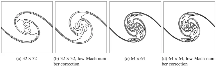
With regard to the low-Mach number regime, the compressible structured-grid framework is not capable of

cap-turing the correct vortex pattern on the 32×32 grid using any of the schemes without a low-Mach number correction.

This is demonstrated in Figures13and14for the MUSCL 5th _{and WENO 9}th_{order respectively. The consequence}

of reducing the Mach number by an order of magnitude is most apparent for the MUSCL 5th_{order scheme. At a grid}

resolution of 64×64, only the WENO 9th_{order scheme is capable of capturing the correct vortex pattern; even the}

MUSCL 5th_{order scheme does not provide the correct vortex pattern at this resolution unless a low-Mach number}

correction is used (Figure13). When the low-Mach number correction is utilized, all schemes are able to provide the

correct vortex pattern even on the coarse 32×32 grid.

The implementation of low-Mach corrections gives a more accurate final vortex structure, specifically on the

32×32 grid, both for the MUSCL 5th(Figure13(b)) and WENO 9thorder (Figure14(b)) schemes; compare the above

results with the ones in Figures7(b)and7(d), respectively. The WENO 9thorder scheme is more resilient to the

low-Mach number dissipation, particularly on the 64×64 grid (Figure14(d)). Within the compressible unstructured-grid

framework, the WENO 5th_{order scheme is found to be sufficiently accurate in capturing the correct vortex pattern at}

low-Mach numbers (Figure15) without requiring the use of either a low-Mach number correction or preconditioning,

even at the lowest grid resolution.

For the compressible Lagrange-Remap framework a 3rd _{order scheme is capable of resolving the two merged}

vortices even on the coarse 33×33 grid (Figure12). Comparing all numerical frameworks with respect to the vortex

evolution patterns over time, the following conclusions can be drawn:

1. At the lowest grid resolution (32×32) the incompressible framework appears insensitive to spatial discretization

higher than 5thorder. In the compressible structured- and unstructured-grid frameworks a gradual improvement

in the results occurs as the order of the numerical schemes is increased.

a 3rdorder numerical scheme on the 33×33 grid. All the other numerical frameworks require greater resolution,

higher-order spatial discretisation, or a combination of both.

3. The only compressible framework that provides the correct vortex pattern in the low Mach regime on a 32×32

grid resolution without any low-Mach number correction or preconditioning is the unstructured-grid, but only

when the WENO 7thorder scheme is employed. This can be attributed to the fact that compressible

unstructured-grid is the only numerical framework, where the reconstruction is carried out using characteristic variables and

thekth-order WENO schemes of this framework entails the use of the non-linear combination of (k−1)-order

reconstruction polynomials ([25,26]) rather than lower-order polynomials as it is the case with the WENO

formulation in the structured-grid framework [17].

4. High-order WENO schemes on a 64×64 grid resolve more flow features than the 3rd _{order compressible}

Lagrange-Remap framework; see Figures6,8,10-11and12for the incompressible structured-grid,

compress-ible structured-grid, compresscompress-ible unstructured-grid and compresscompress-ible Lagrange-Remap methods, respectively.

5. The compressible structured-grid framework provides sharper and more detailed (better resolved) vortex

pat-terns than the incompressible structured-grid framework for the same scheme and spatial-order of accuracy.

6. The “legs” of the mixing layer are resolved by approximately 1-3 cells irrespective of the grid resolution used.

The MUSCL scheme typically requires two to three cells to resolve the “legs” of the mixing layer, while the

WENO scheme requires only one to two cells.

(a) UPWIND 3rd (b) MUSCL 5th (c) WENO 5th (d) WENO 9th

(a) UPWIND 3rd (b) MUSCL 5th (c) WENO 5th (d) WENO 9th

Figure 6:Incompressible structured-gridframework using various limiters on a 642_{grid resolution at timet=6.0 s.}

(a) MUSCL 3rd _{(b) MUSCL 5}th _{(c) WENO 5}th _{(d) WENO 9}th

Figure 7:Compressible structured-gridframework using various limiters on a 322grid resolution at timet=6.0 s.

(a) MUSCL 3rd _{(b) MUSCL 5}th _{(c) WENO 5}th _{(d) WENO 9}th

(a) MUSCL 3rd (b) WENO 3rd (c) WENO 5th (d) WENO 7th

Figure 9:Compressible unstructured-gridframework using various limiters on a 322_{grid resolution for quadrilateral}

mesh at timet=6.0 s.

(a) MUSCL 3rd _{(b) WENO 3}rd _{(c) WENO 5}th _{(d) WENO 7}th

Figure 10:Compressible unstructured-gridframework using various limiters on a 642grid resolution for quadrilateral mesh at timet=6.0 s.

(a) MUSCL 3rd _{(b) WENO 3}rd _{(c) WENO 5}th _{(d) WENO 7}th

Figure 11: Compressible unstructured-gridframework using various limiters on a 642_{grid resolution for Arbitrary}

(a) 33×33 (b) 33×33, Mach=0.02 (c) 65×65 (d) 65×65, Mach=0.02

Figure 12:Compressible Lagrange-Remapframework at different grid resolutions and Mach number 0.2 and 0.02 at timet=6.0 s andt=60.0 s respectively.

(a) 32×32 (b) 32×32, low-Mach num-ber correction

(c) 64×64 (d) 64×64, low-Mach num-ber correction

Figure 13: Compressible structured-gridframework at Mach number 0.02 using the MUSCL 5th order scheme at different grid resolutions.

(a) 32×32 (b) 32×32, low-Mach num-ber correction

(c) 64×64 (d) 64×64, low-Mach num-ber correction

(a) 32×32, Mach=0.2 (b) 32×32, Mach=0.02 (c) 64×64, Mach=0.2 (d) 64×64, Mach=0.02

Figure 15:Compressible unstructured-grid framework using the WENO 5thorder scheme at different Mach number and grid resolutions (Arbitrary Triangular elements).

5.2. Momentum Thickness

The double vortex pairing problem under examination provides an ideal test case for evaluating the performance

of the various numerical schemes and frameworks since the resolved momentum thickness growth from the initial

shear layer is a distinctive characteristic of the mixing in the shear layer. Moreover, a quantitative assessment of the

accuracy of all the schemes can be performed using this metric. As in the previous section commenting on vortex

evolution, all of the numerical frameworks employed are compared against a reference simulation conducted at a grid

resolution of 256×256 in order to ensure that the methods converge to the same momentum thickness growth patterns.

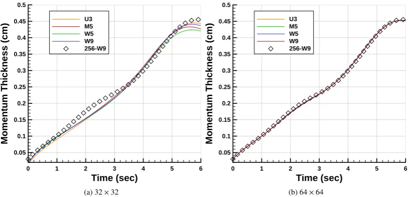
The FSAC-PP method was used to obtain all the results (Figure16) in the incompressible framework. Increasing

the spatial-order of accuracy provided closer agreement with the momentum thickness patterns of the reference

simu-lations. One of the most important observations is that the momentum thickness at the end of the simulationt=6.0 s

is not monotone converging for the 322_{grid as shown in Figure16(a)while it must also be stressed that at the same}

grid resolution, none of the schemes within the incompressible framework agree with the non-linear mixing layer

evolution regime from timet=1.0 s tot=3.0 s of the reference simulation. In contrast, the higher resolution 64×64

grid shows a much better agreement to the reference simulation for all methods, suggesting that at the lower resolution

of 322_{, the effect of the numerical dissipation in conjunction with the initial unresolved interface discontinuity is more}

profound.

With regards to the compressible structured-grid framework, at a 64×64 grid resolution not all schemes are

capable of providing a momentum thickness evolution pattern that is in close agreement to the reference simulation.

In particular, without the low-Mach number correction the momentum thickness is over predicted at late times for

the MUSCL 5th_{order scheme as seen in Figure17(a). The implementation of the low-Mach number correction has}

resulted in an identical temporal growth rate of the momentum thickness at Mach numbers 0.2 and 0.02. Without the

low-Mach number correction the momentum thickness at late times deviates severely from the reference simulation,

For the compressible unstructured-grid framework, the results obtained (see Figure 18) indicate that it is also

sensitive to the numerical scheme and type of grid employed. For the 32×32 quadrilateral grid, the 3rd_{order scheme}

is not capable of resolving the two initial vortices, hence it also under-predicts the momentum thickness at late times.

However, the higher-order schemes such as the WENO 5th_{, provide improved accuracy and the results are therefore}

in closer agreement with the reference simulation. This is due to the fact that at the higher-spatial order of accuracy

both vortices become resolved. On a 32×32 grid using a triangular mesh the results improve dramatically and a good

agreement with the reference simulation is achieved. Furthermore, the non-linear mixing layer evolution between

t=1.0 s andt=3.0 s is well captured by the WENO 5thorder scheme for both grid resolutions employed.

At the 64×64 quadrilateral grid resolution, the only scheme capable of capturing the non-linear mixing layer

evolution is the WENO 5thorder. The triangular meshes can capture this regime with all numerical schemes employed

here apart from the WENO 3rd _{order at the the 32×32 mesh. The compressible unstructured-grid framework is}

sensitive to the spatial-order of accuracy in conjunction with the type of mesh used. Quadrilateral meshes require

higher-order of spatial discretization in order to produce similar results to triangular meshes. This behavior is due to

the non-local character of the reconstruction associated with the quadrilateral stencils that extend to a greater region

on a given mesh than the corresponding triangular ones. Using the WENO 5th_{order scheme on quadrilateral element}

meshes provides the most accurate results. It appears that the most influential parameter that drives the performance of

multi-dimensional reconstruction is not the compactness of the stencils, but the orientation of the cells with respect to

flow features. Consequently, the arbitrary nature of the unstructured triangular meshes proves beneficial for resolving

complicated flow features that are usually arbitrary in terms of orientation and structure. The full mechanism for this

is as yet not fully understood. Another significant feature of the compressible unstructured-grid framework is that the

WENO 5th_{order scheme provides sufficient accuracy to obtain the same momentum thickness evolution pattern as}

the reference simulation in the low-Mach number regime (Figure18) even without resorting to low-Mach correction

or preconditioning.

For the compressible Lagrange-Remap framework (Figure19) the momentum thickness calculated on the 33×33

grid is under-predicted. Using a 65×65 grid resolution, a closer agreement with the reference simulation is achieved

(Figure 19). Although the momentum thickness on the 65×65 grid resolution is quite similar to the reference

simulation, the non-linear mixing layer evolution regime from timet=1.0 s tot=3.0 s is under-predicted. The same

trend also occurs during the very low-Mach number simulation, where good agreement with the reference simulation

is achieved (hardly distinguishable from the reference simulation at Mach number of 0.2).

The main conclusions regarding the accuracy of different numerical frameworks with respect to the momentum

1. The prediction of momentum thickness is sensitive to the spatial-order of accuracy with higher accuracy achieved

when increasing the order of accuracy.

2. The compressible unstructured-grid framework is capable of capturing the momentum thickness evolution at

low-Mach number even without the use of a low-Mach number correction or preconditioning.

3. The compressible structured-grid framework is prone to low-Mach dissipation, except the case of WENO 9th

order scheme on the 64×64 grid.

4. All the schemes, in all the frameworks provide non-monotone converging results for momentum thickness

towards the end of the simulation. This indicates a dependence upon the initial conditions varying with the grid

resolution;

5. The most difficult pattern to accurately capture at the coarsest resolution (32×32) is the non-linear mixing layer

regime betweent =1.0 s andt =3.0 s. This is indicative of the secondary eigenmode of the initial condition

associated with the second wavenumberk2and the formation of the two pairing vortices.

Time (sec)

M

o

m

e

n

tu

m

T

h

ic

k

n

e

s

s

(

c

m

)

0 1 2 3 4 5 6

0.05 0.1 0.15 0.2 0.25 0.3 0.35 0.4 0.45 0.5

U3 M5 W5 W9 256-W9

(a) 32×32

Time (sec)

M

o

m

e

n

tu

m

T

h

ic

k

n

e

s

s

(

c

m

)

0 1 2 3 4 5 6

0.05 0.1 0.15 0.2 0.25 0.3 0.35 0.4 0.45 0.5

U3 M5 W5 W9 256-W9

(b) 64×64

Time (sec) M o m e n tu m T h ic k n e s s ( c m )

0 1 2 3 4 5 6

0.05 0.1 0.15 0.2 0.25 0.3 0.35 0.4 0.45 0.5 M5 M5 LM M5 Mach=0.02 M5 Mach=0.02 LM 256-W9

(a) MUSCL-5th

Time (sec) M o m e n tu m T h ic k n e s s ( c m )

0 1 2 3 4 5 6

0.05 0.1 0.15 0.2 0.25 0.3 0.35 0.4 0.45 0.5 W9 W9 LM W9 Mach=0.02 W9 Mach=0.02 LM 256-W9

(b) WENO-9th

Figure 17: Momentum thickness in time for thecompressible structured-grid framework using various numerical schemes and Mach number on the 642grid.

Time (sec) M o m e n tu m T h ic k n e s s ( c m )

0 1 2 3 4 5 6

0.05 0.1 0.15 0.2 0.25 0.3 0.35 0.4 0.45 0.5 32x32 W3 32x32 W5 64x64 W3 64x64 W5 256 W7 (a) Quadrilateral Time (sec) M o m e n tu m T h ic k n e s s ( c m )

0 1 2 3 4 5 6

0.05 0.1 0.15 0.2 0.25 0.3 0.35 0.4 0.45 0.5 32x32 W3 32x32 W5 64x64 W3 64x64 W5 256 W7 (b) Triangular

Time (sec)

M

o

m

e

n

tu

m

T

h

ic

k

n

e

s

s

(

c

m

)

0 1 2 3 4 5 6

0.05 0.1 0.15 0.2 0.25 0.3 0.35 0.4 0.45 0.5

33x33 Mach=0.2 65x65 Mach=0.2 65x65 Mach=0.02 257-LR

Figure 19: Momentum thickness variation in time for thecompressible Lagrange-Remapframework using various grid resolutions and Mach numbers.

5.3. Numerical Dissipation

The viscous dissipationDV (equation (17)) and kinetic energy loss rateDKE (equation (16)), or total dissipation,

provide the means to investigate the numerical dissipationDN(equation (18)) of each computational framework at the

various grid resolutions. In the incompressible case,DKErepresents the total dissipation rate (viscous plus numerical).

In the compressible cases,DKErepresents the total dissipation rate on average, but there is superimposed oscillatory

behavior due to acoustic vibrations, as will be discussed later. An example showcasing the contribution of each

dissipation component is given in Figure20. The dissipation density (per volume) in Figures20-26is measured in

kg/(m·s3_).

In the incompressible simulations at the 32×32 resolution, the numerical dissipation of the 3rd _{order upwind}

scheme initially has lower values, while the MUSCL 5th, WENO 5thand 9th order schemes have a higher numerical

dissipation that reduces, however, at a faster rate (Figure21(a)). At 64×64 (Figure21(b)) resolution the dissipation

changes similarly for all schemes, leading to the conclusion that the numerical reconstruction has a little influence on

the incompressible FSAC-PP method.

For the compressible structured-grid framework at 32×32 resolution (Figure22) it is evident by comparing the

MUSCL 5th_{(Figure22(a)) and WENO 9}th_{(Figure22(b)) order schemes that the numerical dissipation is reduced as}

the spatial order of accuracy is increased, thus obtaining a closer agreement with the reference simulation.

The oscillatory behavior of the numerical dissipation at Mach number of 0.2 is due to acoustic vibrations.

Reduc-ing the Mach number value to 0.02 significantly reduces the oscillations. EmployReduc-ing the low-Mach number correction

Time (sec) D is s ip a ti o n

0 1 2 3 4 5 6

0 4E-06 8E-06 1.2E-05 1.6E-05 2E-05 Total Viscous Numerical

(a) 322MUSCL 5th

Time (sec) D is s ip a ti o n

0 1 2 3 4 5 6

0 4E-06 8E-06 1.2E-05 1.6E-05 2E-05 Total Viscous Numerical

(b) 642MUSCL 5th

Time (sec) D is s ip a ti o n

0 1 2 3 4 5 6

0 4E-06 8E-06 1.2E-05 1.6E-05 2E-05 Total Viscous Numerical

(c) 322WENO 9th

Time (sec) D is s ip a ti o n

0 1 2 3 4 5 6

0 4E-06 8E-06 1.2E-05 1.6E-05 2E-05 Total Viscous Numerical

(d) 642WENO 9th

Figure 20: Comparison of totalDKE, viscousDV and numericalDN dissipation for the MUSCL 5thand WENO 9th

order schemes on the 322_{and 64}2_{grids in thecompressible structured-gridframework.}

(Figure23) grid resolutions for almost all schemes. Specifically, all schemes are found to have a better match to the

reference solution when utilizing the low-Mach number correction, except the WENO 9th_{order scheme for which no}

tangible changes appear.

Using the compressible structured-grid finite volume solver to perform ILES of a turbulent plane channel flow

[50], it was observed that the low-Mach number correction in conjunction with the WENO 9th_{order scheme had an}

adverse effect on the accuracy of the solution, similar to what is observed herein. However, the results on the very

coarse grid (32×32) actually show an improvement when using the low-Mach number correction with the WENO

9th order scheme suggesting that there is a more complex interaction of the numerical terms. This is demonstrated

qualitatively by the improvement in the structure and resolved features of the final vortex compared to the cases;

compare the results with and without low-Mach correction in (Figure14(b)) and (Figure14(a)), respectively, as well

dissipation is significantly reduced during the first second of the double vortex instability development. Hence, in

under-resolved simulations encompassing significant numerical dissipation the use of the low-Mach correction is

likely to prove overall beneficial.

Figure23presents the numerical dissipation on the 64×64 grid for the compressible structured-grid framework.

The comparison of the results in Figures23(a)and23(b)show that for Mach number of 0.2 the MUSCL 5th _order

scheme is only slightly more dissipative than the WENO 9th_{order. However, the difference between the two schemes}

becomes more apparent when reducing the Mach number to 0.02. The WENO 9thorder shows hardly no difference

to the (average) dissipation values obtained at Mach number of 0.2. The implementation of the low-Mach number

correction at a Mach number of 0.2 manages to marginally reduce the numerical dissipation of the MUSCL 5thorder

scheme (Figure23(a)). At a Mach number of 0.02, however, the reduction of numerical dissipation is even more

profound. The difference in the results of the WENO 9th _{order scheme with and without low Mach correction are}

practically indistinguishable (Figure23(b)).

For the compressible unstructured-grid framework at 32×32 resolution (Figure24) the numerical dissipation

relies on the spatial-order of accuracy of the scheme throughout the simulation. As the spatial-order of accuracy is

increased, a closer agreement with the reference simulation is obtained. All the numerical reconstructions exhibit

the oscillatory dissipation behavior. At the 64×64 grid resolution, the numerical dissipation (DN) approaches zero

much faster at early times comparing to the remaining computational approaches, while simultaneously the oscillatory

behavior becomes less pronounced, especially when using triangular shaped elements (Figure25).

For a structured (quadrilateral) mesh, the numerical dissipation of the compressible structured-grid framework

using the WENO 9th order scheme and that of the compressible unstructured-grid framework using the WENO 5th

order scheme (multi-dimensional stencil) are very similar (Figure25). However, for (arbitrary) triangular elements

the compressible unstructured-grid framework exhibits significantly lower numerical dissipation, particularly during

the first few seconds of the vortex evolution, where the two pairing vortices develop. To some extent this explains why

the compressible unstructured-grid framework is capable of obtaining the most accurate final vortex structure at the

very low-Mach number of 0.02 discussed in§5.1and Figure15; the compressible-unstructured framework is able to

adequately resolve the secondary instability (second eigenmode in equation (3)), which develops into the two pairing

vortices, as a result of the very low numerical dissipation.

Similar to other methods, in the compressible Lagrange-Remap framework the numerical dissipation (DN) reduces

with increasing the mesh size (Figure26). However, the values of the numerical dissipation (DN) attained at early

times are significantly lower than any of the other compressible frameworks. The oscillations witnessed in the the

reduced at the Mach number of 0.02.

Comparing all the numerical frameworks with respect to the numerical dissipation lead to the following

conclu-sions:

1. The oscillatory behavior of the numerical dissipation (DN) is a consequence of the oscillations present in the

total dissipation (DKE) as shown in Figure 20. These oscillations occur only in the compressible solutions

due to acoustic (compressible) effects as demonstrated in Figure26(b). At 2562_{resolution, the numerical}

dis-sipation is almost purely comprised of the ”resolved” acoustic fluctuation, as it is evident by the very close

agreement between the different compressible frameworks, particularly aftert=1sec. An almost perfect

agree-ment is obtained between the compressible structured- and unstructured-grid frameworks. In the compressible

Lagrange-Remap framework a good agreement is present at early times, however, a phase difference is evident

at late times.

2. At 32×32 grid resolution, the compressible unstructured-grid framework provides the best agreement with

the reference simulation. As the spatial order of accuracy is increased a better agreement is achieved even at

earlier times. This can be attributed to the fact that the present framework utilizes the (k−1) order polynomials

for akthorder accurate schemes, and that the same polynomials are used for the approximation of the velocity

and temperature gradients in the viscous fluxes. For comparison, both the incompressible and compressible

structured-grid frameworks use a 2nd order central approximation of the temperature and velocity derivatives

in the viscous fluxes and are thus second order accurate. Clearly, there is a benefit of employing higher-order

approximations for the viscous part of the equations.

3. The compressible Lagrange-Remap framework provides a closer agreement with the reference simulation at

Time (sec) N u m e ri c a l D is s ip a ti o n

0 1 2 3 4 5 6

0 5E-06 1E-05 1.5E-05 2E-05 2.5E-05 U3 M5 W5 W9 256-W9

(a) 32×32

Time (sec) N u m e ri c a l D is s ip a ti o n

0 1 2 3 4 5 6

0 2E-06 4E-06 6E-06 8E-06 1E-05 U3 M5 W5 W9 256-W9

(b) 64×64

Figure 21: Numerical dissipation in time for theincompressible structured-gridframework using various numerical schemes and grid resolutions.

Time (sec) N u m e ri c a l D is s ip a ti o n

0 1 2 3 4 5 6

0 5E-06 1E-05 1.5E-05 2E-05 M5 M5 LM M5 Mach=0.02 M5 Mach=0.02 LM 256 W9

(a) MUSCL 5th

Time (sec) N u m e ri c a l D is s ip a ti o n

0 1 2 3 4 5 6

0 4E-06 8E-06 1.2E-05 1.6E-05 2E-05 W9 W9 LM W9 Mach=0.02 W9 Mach=0.02 LM 256 W9

(b) WENO 9th

Time (sec) N u m e ri c a l D is s ip a ti o n

0 1 2 3 4 5 6

0 2E-06 4E-06 6E-06 8E-06 1E-05 M5 M5 LM M5 Mach=0.02 M5 Mach=0.02 LM 256 W9

(a) MUSCL 5th

Time (sec) N u m e ri c a l D is s ip a ti o n

0 1 2 3 4 5 6

0 2E-06 4E-06 6E-06 8E-06 1E-05 W9 W9 LM W9 Mach=0.02 W9 Mach=0.02 LM 256 W9

(b) WENO 9th

Figure 23: Numerical dissipation in time for thecompressible structured-grid framework using various numerical schemes on the 64×64 grid.

N u m e ri c a l D is s ip a ti o n 1E-05 Time (sec) 5E-06

0 2 4 6

M3 W5 W7 256T W7

(a) 32×32

0 M3 W5 W7 256T W7 1E-06 N u m e ri c a l D is s ip a ti o n Time (sec)

2 4 6

0 2E-06

-1E-06

-2E-06

(b) 64×64

Time (s) N u m e ri c a l D is s ip a ti o n

0 1 2 3 4 5 6

-2E-06 0 2E-06 4E-06 6E-06 64T W5 64Q W5

64 W9 LM (Structured)

Figure 25: Numerical dissipation for thecompressible unstructured-gridframework; comparison between Quadrilat-eralvs.Triangular elements.

Time (sec) N u m e ri c a l D is s ip a ti o n

0 1 2 3 4 5 6

-1E-06 -5E-07 0 5E-07 1E-06 1.5E-06 65x65 LR

65x65 LR Mach=0.02 256 LR

(a) Compressible Lagrange-Remap

Time (sec) N u m e ri c a l D is s ip a ti o n

0 1 2 3 4 5 6

-1E-06 -5E-07 0 5E-07 1E-06 1.5E-06 Structured Incompressible Structured Compressible Unstructured Compressible Lagrange-Remap

(b) Reference 2562_{for all frameworks}

Figure 26: Numerical dissipation for thecompressible Lagrange-Remapframework on the 64×64 grid resolution as well as for all frameworks on the 256×256 reference grid resolution. The oscillations are a manifestation of acoustic fluctuations associated with compressibility effects (see Sec. 5.3 for further discussion).

5.4. Computational Efficiency

The evolution of momentum thickness in time (see§5.2) indicated the presence of a non-monotone converging

behavior towards the end of the simulation (t=6.0sec). Therefore, to assess numerical efficiencyvs.error reduction,

we have chosen to measure the average percentage of the momentum thickness error from the reference solution (of

computational time, which is chosen to be the fastest simulation of each individual framework. Typically, this is the

simulation time of the first-order scheme employed at grid resolution (32×32).

The error is calculated by:

Error%= 1

T T Z

t=0

|θ_S(t)−θ_R(t)|

θR(t)

dt ×100% (19)

where the momentum thicknessθ(t) is given by equation (15). The termθS refers to the values obtained from the

under-resolved simulations, whileθRstands for each numerical framework reference simulation on the 256×256 grid.

T is the total simulation time, which isT =6 sec andT =60 sec for the Mach numbers of 0.2 and 0.02, respectively.

In Figure 27, equation (19) is used to obtain an error estimate for each scheme on the 322 and 642 grids. The

results are plotted against the normalized total simulation time, as detailed above, in order to highlight the efficiency

of each numerical scheme as the order of accuracy increases.

Figure27reveals that:

1. Increasing the spatial order of accuracy reduces the numerical error; this applies to all computational

frame-works employed here.

2. In the incompressible structured-grid framework, the WENO methods provided the most optimal convergence

rate (Figure27(a)).

3. For the compressible structured-grid framework (Figure27(b)), the low-Mach number correction significantly

improves the accuracy of all schemes apart from the WENO 9th _{order. This indicates that for very high-order}

schemes and at a sufficient grid resolution, the low-Mach number correction may not provide any further

bene-fits.

4. The error of the compressible unstructured-grid framework (Figure27(c)) is dependent both on the mesh type

and numerical scheme employed. In general, grids comprising triangular cells reduce the error faster than the

corresponding quadrilateral grids.

5. The compressible Lagrange-Remap (Figure27(d)) is the fastest of all computational frameworks employed in

this study, although the slope of the error reduction as a function of computational time is not as steep as for

some of the other methods.

6. The lowest errors at both grid resolutions are obtained with the compressible unstructured-grid framework.

This is traded against their computational expense associated with the multidimensional nature of the

recon-struction, high-order quadrature surface and volume integral, as well as with the indirect data accessing due to