Reliability modeling of a 1-out-of-2 system: Research with diverse Off-the-shelf SQL database servers

(1)

City, University of London Institutional Repository

Citation

: Bishop, P. G., Gashi, I., Littlewood, B. and Wright, D. (2007). Reliability

modeling of a 1-out-of-2 system: Research with diverse Off-the-shelf SQL database servers.

Paper presented at the The 18th IEEE International Symposium on Software Reliability

(ISSRE '07), 5 - 9 Nov 2007, Trollhättan, Sweden.

This is the unspecified version of the paper.

This version of the publication may differ from the final published

version.

Permanent repository link:

http://openaccess.city.ac.uk/520/

Link to published version

:

Copyright and reuse:

City Research Online aims to make research

outputs of City, University of London available to a wider audience.

Copyright and Moral Rights remain with the author(s) and/or copyright

holders. URLs from City Research Online may be freely distributed and

linked to.

City Research Online:

http://openaccess.city.ac.uk/

[email protected]

(2)

ᑨ

睴

诲睸睺睺

Ơ

″

Reliability Modeling of a 1-Out-Of-2 System: Research with Diverse

Off-The-Shelf SQL Database Servers

Peter Bishop

1, 2

, Ilir Gashi

1

, Bev Littlewood

1

and David Wright

1

_{Centre for Software Reliability, City University,}

2

_{Adelard LLP}

orthampton Square orthampton Square

London, EC1V 0HB London, EC1V 0HB

E-mail: [email protected], [email protected], {bl, d.r.wright}@csr.city.ac.uk

Abstract

Fault tolerance via design diversity is often the only viable way of achieving sufficient dependability levels when using off-the-shelf components. We have reported previously on studies with bug reports of four open-source and commercial off-the-shelf database servers and later release of two of them. The results were very promising for designers of fault-tolerant solutions that wish to employ diverse servers: very few bugs caused failures in more than one server and none caused failure in more than two. In this paper we offer details of two approaches we have studied to construct reliability growth models for a 1-out-of-2 fault-tolerant server which utilize the bug reports. The models presented are of practical significance to system designers wishing to employ diversity with off-the-shelf components since often the bug reports are the only direct dependability evidence available to them.

1. Introduction

Off-the-shelf (OTS) components are used ubiquitously in software systems development due to the perceived lower costs from their use (some of the components may be open-source and/or freely available), faster deployment and the multitude of available options. There remain concerns, however, about the dependability levels of the components: they tend to be distributed without any assurances of their dependability, with “use-as-is” labels often attached to them by the vendors. As a result, the only viable way available to users and system integrators of achieving higher dependability is to use software fault tolerance. Fault tolerance may take multiple forms, with examples ranging from simple error detection and recovery add-ons (e.g. “wrappers” [1]) to “diverse modular

redundancy” (e.g. “N-version programming”: replication with diverse versions of components) [2].

The design decisions are well known from the literature. But, questions remain about the dependability gains that developers of systems using OTS components can expect, the implementation difficulties and the extra cost expected. We have studied some of these issues with OTS database servers or database management system (DBMS) products: a complex category of OTS products. The architectural solutions for implementing a fault-tolerant DBMS using diverse OTS database products are given in [3].

With regard to the dependability of a fault tolerant DBMS, we have reported previously on a study with the publicly available fault reports of four OTS DBMS products (both open-source and closed development) [4] and later releases of two of them [3]. We found that a high number of these faults would not be tolerated (or even detected) by the existing non-diverse fault-tolerant schemes but did not cause failures in any two diverse DBMS products. We found the number of faults that caused coincident failures to be very low. These results seem to suggest that significant dependability gains may be achieved if diverse modular redundancy is employed with OTS DBMS products. However they are not definitive evidence. The main problem is that the available reports concern faults (bugs) and not how many failures each caused, which makes their use in reliability predictions difficult. Complete failure logs would be much more useful as statistical evidence, but they are not available. The only direct dependability evidence available for these products often are the fault reports.

(3)

ᑨ

睴

诲睸睺睺

Ơ

4 Ơ ″

can we incorporate existing evidence for off-the-shelf products to evaluate the possible gains in reliability achievable by a 1-out-of-2 diverse server?” To this end we have studied two approaches which use fault reports for obtaining dependability measures of a fault tolerant server employing two diverse OTS DBMS products For the sake of brevity, we shall refer to this fault tolerant DBMS as a “FT-node”.

The two approaches presented in this paper for estimating the reliability of a FT-node are:

1. An extension of a previous software reliability growth model [5] for use in reliability growth modeling of the FT-node.

2. An alternative “proportions” approach where the observed reliability of a single server is scaled by a factor to derive the expected reliability of the FT-node.

The first method requires information on actual usage time. In closed development environments, it should be feasible to derive usage time from dated fault reports if the total population of the DBMS product is known over time (e.g. from product registration). However for open source products, information on the product population over time is hard to obtain, and hence the usage time is difficult to estimate.

We have therefore developed a second method where information about usage time is not required and statements about the reliability improvement achievable by an FT-node can be made (under certain assumptions about the underlying failure rate distributions), based only on information derived from reported product faults.

The paper is structured as follows: section 2 contains background on the studies we have conducted with known fault reports of the DBMS products, software reliability growth modeling and the Littlewood [5] model; section 3 details the extensions of the Littlewood model [5] for the reliability growth modeling of the FT-node; section 4 contains details of an alternative model in which fault counts alone are used for reliability prediction of the FT-node; in the same section we also provide empirical data to illustrate the use of the method; section 5 contains a discussion and verifications of the main modeling assumptions made and finally section 6 contains a discussions of the two modeling approaches, conclusions and provisions for further work.

2. Background and related work

2.1 Analysis of faults in OTS DBMS products

We have conducted two studies with fault reports of four OTS DBMS products and later releases of two of

them. We have fully described these studies and provided analysis of the results in [4] and [3]. We will be utilizing the results of those studies in this paper as empirical evidence with one of the models, as well as for verification of assumptions. Therefore, in what follows we will provide a brief summary of the studies and the main results.

A mixture of free open-source and commercial closed development products were used in the studies. In the first study we collected a total of 181 bugs reported for the following DBMS products, of which the first two are open-source and the last two are commercial closed-development products (for the sake of brevity, we will use the abbreviations detailed in brackets next to each product when referring to these products from this point forward):

- Interbase 6.0 (IB) - PostgreSQL 7.0 (PG7.0) - Oracle 8.0.5 (OR)

- Microsoft SQL Server 7 (MS).

We first ran the bug scripts (contained within the bug reports) on the products for which they were reported and then (when possible1) on the other products. We found very few bugs that caused coincident failures in more than one DBMS product, and none which caused failure in more than two.

The results were encouraging, but they only represented one snapshot in the evolution of these products. Therefore we repeated the study for the later releases of the two open-source products (due to difficulties with data collection no new bug reports were collected for the commercial products):

- Firebird 1.0 (FB) (this is the open-source descendant of Interbase 6.0)

- PostgreSQL 7.2 (PG7.2)

We collected 92 new bugs reported for these two products. The results of the second study substantially confirmed those of the first: very few bug reports caused coincident failures. This suggests that factors that make diversity useful do not disappear as the DBMS products evolve and is a further indication that diversity with OTS products certainly deserves further study.

2.2 Software reliability growth modeling

Software reliability growth modeling is a well studied subject over the previous thirty years. A good reference to the subject is [6]. Chapter three of [6]

1

(4)

provides a comprehensive survey of the well known models. In what follows we will provide details of one of these models which has been extended in this paper.

2.3 Littlewood model

In what follows we will use the notation and assumptions first described in the Littlewood model [5]. In [5] (and in reliability growth modeling in general), interest centers upon time-to-failure distributions and the data is a sequence of successive execution times between the failures t1, t2, … ti. The

following assumptions are made:

1. Each of the (the number of faults that exist in the OTS software product at its release) faults will cause a failure after a time which is distributed exponentially, and independently of other faults, with rate Φi,

where Φ1, …, Φ are independent identically distributed (i.i.d.) random variables,

2. When a failure occurs, there is an instantaneous removal of the fault which caused the failure, 3. If a total time τ has elapsed and i faults have been

removed and Φ1, … , Φ-i are the failure rates of the

remaining (latent) faults, then the failure rate of the program is the sum of the rates of these remaining faults (the indices will require renumbering) Λ = Φ1

+ … + Φ-i

4. When debugging starts each Φi has the probability

density function (pdf) b Γ (bφ; a), the Gamma Distribution with parameters2a and b, with φ being the realization of the random variable Φi.

Following on from these assumptions it is shown in [5] that the times, Ti, at which the faults show

themselves are i.i.d. random variables and they are

Pareto distributed: P(Ti< t) = a

t

b

)

(

1 +

−

(1)

The motivation behind these assumption and the full details of the model can be found in [5].

3. Extending the Littlewood model

In this section we discuss how the Littlewood model can be extended for reliability growth modeling of a 1-out-of-2 FT-node (i.e. the FT-node is assumed to fail only if both of its components fail on a particular demand).

2

We defined the parameters of the gamma Distributions as a (shape) and b (scale) instead of the conventional α and β since we will define β for a different purpose in section 4.

The assumptions described in section 2.3 are retained, but some additional assumptions are necessary to make the analysis tractable. We assume that:

1. The operational profiles (averaged over all users) of the two different DBMS products are the same. 2. There are three different fault totals

AB B A B

A

, , of faults initially present in the software that cause failure in A-only, B-only or both A and B. The times to discovery of these faults will still be assumed to be conditionally exponentially distributed random variables given the failure rate distribution, but the failure rate may be different for each fault.

3. Failure due to a specific fault is reported once only, for each product version in which it occurs.

4. The failure rate distributions for each of the

AB B A B

A Φ Φ

Φ , , (for the three different types of failures that the faults cause) are assumed to be drawn from the same gamma distribution (we will discuss this assumption in more detail in section 5). Based on these assumptions, an extended Likelihood function of the Littlewood model has been derived (see Appendix A). This model makes use of the observed failure times of a given type in products A and/or B.

Clearly to apply the model, it is necessary to have data on the inter-failure times. If the DBMS suppliers maintain detailed information about the calendar time when the fault was reported (this is usually available) and data on the number of installed versions over time, then calendar time can be scaled to derive the total product usage time between failures.

Knowledge of the installed base is only usually known to “closed source” DBMS product vendors where each instance of the software is licensed. Such data is not usually publicly available, but in principle inter-failure times can be estimated.

Quantifying the usage time for open-source OTS software products is more difficult. A possible proxy for the installed base is the number of downloads [7], however there are many uncertainties including:

- Multiple download sites and/or mirrors exist for each product

- OTS products are often distributed as part of operating systems

- Downloaded products may not actually be used. Due to these difficulties, we have not yet obtained the data needed to apply the extended Littlewood model (although it may be feasible in the future, especially for closed source products).

(5)

4. The proportions approach

In this section we will explain a different approach which attempts to get away from the need to quantify actual usage time between failures. This alternative approach is useful in applications where it may be difficult to quantify the usage time, and hence difficult to use the model described in Section 3.

The alternative approach to modeling the reliability of a 1-out-of-2 FT node is to use:

- the counts of faults which are available from the fault logs of each product. From it we can then calculate the proportion of faults in product Athat are also found to cause failure in product B, βAB,

(from the ratio of common to non-common faults in the fault history of A). Similarly we can also calculate βBA for product B faults that are also found

to cause failure in A.

- the pfd (probability of failure on demand) of the products A and/or B; estimates of these may exist for a particular application based on actual failures in operation for that application

This approach has the following underlying assumptions:

- Common faults are drawn from the same failure rate distribution as non common faults, i.e. a constant proportion of faults in each failure rate band are common to A and B.

- The failure rate distributions for A and B are the same.

These assumptions are identical to those made for the extension to the Littlewood model described in section 3. Given these assumptions, we can estimate the

expected common mode failure rate as: E(λAB) = βAB E(λA) or

E(λBA) = βBA E(λB)

Where E(λAB) and E(λBA) both represent common mode failure rate estimates that should be, in principle, equivalent. In what follows we will describe in more detail how these two expressions were obtained.

4.1. The underlying theory of the proportions

approach

Fault density, h(φ), represents the number of faults within a given failure rate interval that remain in a component. So, component fault-count and failure rate

are given by

∫

∞

=

0

)

(

φ

d

φ

h

and

∫

∞

=

0

)

(

φ

λ

h

d

respectively.

We assume the fault density functions of the A, B and AB fault classes are:

h(φ)Α = ΝΑp(φ) (2)

h(φ)Β = ΝΒp(φ) (3)

h(φ)ΑΒ = ΝΑΒp(φ) (4)

where:

ΝΑis the total number of faults in Product A

ΝΒis the total number of faults in Product B

ΝΑΒare faults common to Products A and B

p(φ) is the probability distribution3 of failure rate φ for a fault in the product (assumed to be the same for A, B and AB faults).

Note that A and B here are the total number of

faults in each product (i.e. _A=_A_B +_AB and

AB B A

B

= + )

Under these assumptions, the expected number of those faults nA,τΑ observed in product A during usage

until time τΑis:

E(nA,τΑ ) = ΝΑ (1 −

∫

∞ −

0

)

(

φ

e

φτ

d

φ

p

A ) ₍₅₎

The expected value of the number of faults nAB,τΑ

observed in product A during usage until time τΑ that

are also common to product B is: E(nAB, τΑ) = ΝΑΒ (1 −

∫

∞ −

0

)

(

φ

e

φτ

d

φ

p

A ) ₍₆₎

It can be seen that the assumption of a common failure rate distribution means that the bracketed term (the probability a fault is found after time τΑ) is

identical for E(nA) and E(nAB) and will cancel out if we

take the ratios. So knowledge of the actual usage time

τΑand the failure rate distribution p(λ) is not required.

So we can estimate βΑΒfrom the fault sequence

observed in product A up to τΑ, where some faults in

the sequence are labeled as being common to B (from a knowledge of the B product faults). Given the observed values, nA,τΑand nAB,τΑ:

βΑΒ = ΝΑΒ /ΝΑ ∼ nAB,τΑ / nA,τΑ (7)

Similarly, we can also estimate βΒΑfrom the fault

sequence observed in product B up to τΒ

βΒΑ = ΝΑΒ /ΝΒ ∼ nBA,τΒ / nB,τΒ (8)

These βvalues need not necessarily be identical as one product could contain more faults than another.

If we now consider the use of a product for a particular application, the operational profile is likely to differ from the average usage profile for the product

3 _{We use λ for the failure rate of an entire}

(6)

which determines the average failure rate distribution p(φ). For a different usage profile there will be a new failure rate distribution p(φ)′. However if common faults are randomly chosen from the set of available faults, there is no reason to believe that the proportion of common faults will change for any given failure rate

φ), i.e. we assume that:

h(φ)′Α = ΝΑp(φ)′ (9)

h(φ)′ΑΒ = ΝΑΒp(φ)′ (10)

So the expected failure rates are:

E(λΑ) = ΝΑ

∫

∞

′

0

)

(

φ

d

φ

p

(11)

E(λΑΒ) = ΝΑβ

∫

∞

′

0

)

(

φ

d

φ

p

(12)

and hence:

E(λΑΒ) = βΑΒ Ε(λ A) (13)

and similarly:

E(λ ΒΑ) = βΒΑ Ε(λ B) (14)

The estimates of the performance of each DBMS product, E(λA) and E(λB) are derived from testing or

standalone operation for the actual application, and the

βvalues are estimated from the bug history.

In practice, the estimates E(λΑΒ) and E(λΒΑ) are

likely to differ due to uncertainties in the β and

λ values and, in this case, the most conservative estimate should be used.

4.2 Empirical derivation of

ββββ

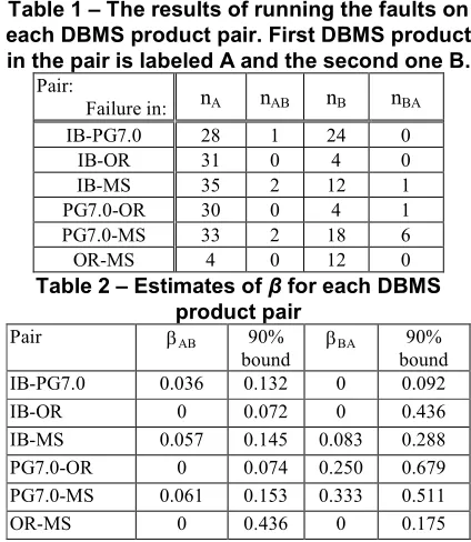
In this section we will use the results of our previous studies with the bugs [4], [3] (which we summarized in section 2.1) to derive empirical estimates of β. The results of the first study from running the DBMS product faults that could be run on each pair and the failures that they cause are given in Table 1:

- nAare faults reported in product A

- nAB are product A reported faults that also affect B

- nBare faults reported in product B

- nBA are product B reported faults that also affect A.

The results presented in Table 1 do not distinguish between “Bohrbugs” and “Heisenbugs”4, i.e. we assume the fault will always cause a failure in the DBMS product for which it was reported (but not, unless it does cause a failure, for other products) even

4

Terms introduced by Gray [8], defining two types of bugs: “Bohrbugs” appear to be deterministic (the failures they cause are easy to reproduce in testing); “Heisenbugs”, are difficult to reproduce as they only cause failures under special conditions: "strange hardware conditions (rare or transient device fault), limit conditions (out of storage, counter overflow, lost interrupt, etc.) or race conditions"

if when we tested it in our setup we did not observe the failure that was detailed in the bug report. The β values obtained for this dataset are given in Table 2.The table also contains 90% upper confidence bounds on the estimates. The confidence bound is computed using:

Pr(β < p |n,x) = ∑r=0,x..C(n,r)pr(1-p)n-r (15)

[image:6.595.72.285.179.334.2]

where x is the number of common faults in a sequence of n faults.

Table 1 – The results of running the faults on each DBMS product pair. First DBMS product in the pair is labeled A and the second one B.

Pair:

Failure in: nA nAB nB nBA

IB-PG7.0 28 1 24 0

IB-OR 31 0 4 0

IB-MS 35 2 12 1

PG7.0-OR 30 0 4 1

PG7.0-MS 33 2 18 6

OR-MS 4 0 12 0

Table 2 – Estimates of β for each DBMS product pair

Pair βΑΒ 90%

bound

βΒΑ 90%

bound

IB-PG7.0 0.036 0.132 0 0.092

IB-OR 0 0.072 0 0.436

IB-MS 0.057 0.145 0.083 0.288

PG7.0-OR 0 0.074 0.250 0.679

PG7.0-MS 0.061 0.153 0.333 0.511

OR-MS 0 0.436 0 0.175

Note that the number of faults for a product (like IB) is not constant for different partners (like PG7.0 and MS) as it only includes the subset of faults that can be run on the product pair.

The β values vary considerably for the different product pairs but the number of common faults is low (and sometimes zero) so the estimation errors are large. From equations (7) and (8), it can be seen that the βΒΑ,

βΑΒ values need not be identical as they depend on the

number of residual faults, NA and NB, which can vary

with the quality of the development process. However many of the βΒΑ, βΑΒ values for the DBMS product

pairs seem to be similar given the inherent sampling errors. The main exceptions to this observation are the

PG7.0-MS and PG7.0-OR DBMS product pairs where the βΒΑ value exceeds the 90% confidence bound

estimate for the βΑΒ value. The proportions theory

indicates that this would occur if PG7.0 had significantly more residual faults than OR and MS.

[image:6.595.310.522.200.444.2]

(7)

10 fold or more compared with a single DBMS product.

We also compared β values for successive versions of the same DBMS product pairs using the results from our second study [3] (described in section 2.1). These can be compared with the faults found in the earlier releases. The results are given in Table 3.

Table 3 - The results for different releases

Pair:

Failure in: nA nAB nB nBA

IB-PG7.0 28 1 24 0

FB-PG7.2 30 1 18 1

The β factor estimates for earlier and later releases of the products are given in Table 4.

Table 4 - β values for different releases

Pair βΑΒ 90% bound βΒΑ 90% bound

IB-PG7.0 0.036 0.132 0.000 0.092 FB-PG7.2 0.033 0.124 0.056 0.200

The β values seem relatively consistent between different releases of the same product pair (around 0.035). This might indicate that the relative improvement can be estimated from previous releases of the DBMS product pairs (where more data may be available). However it is difficult to draw any firm conclusions due to the high uncertainty in the estimations.

5. Validity of assumptions

The two underlying assumptions of both the approaches that have been discussed in this paper are that: the failure rate distributions for A and B are the same; the failure rate distribution of AB-faults is also the same as those of A and B. The following subsections consider whether these assumptions are credible, and present some statistical tests of the underlying assumptions.

5.1 Similar

failure

rate

distribution

assumption

There is some justification for believing the assumption that the failure rate distributions for the DBMS product pairs are the same. The research by Adams [9] shows that there is remarkable consistency in the failure rate distributions of different operating systems from the same supplier. In addition, in previous work by one of the authors of this paper [10], it was argued that the failure rate distribution is determined by the complexity of the program structure and the failure rates are likely to have the same (log-normal) distribution. This theory is consistent with the empirical observations in Adams [9].

5.2 Conservatism of the common failure rate

assumption

It is also assumed that AB faults have the same distribution as the A and B faults. This would be the case if the AB faults are not “special” in any way (i.e. the AB faults are chosen at random from the set of A faults). For the empirical results presented in section 4.2, the AB faults chosen differed for each DBMS product pair. So no faults were observed that were common to three products (i.e. there are no “special” AB faults that occur very frequently). This gives some credence to the idea of random selection (as a bias towards selecting the same common faults should make triple common faults more likely).

We also note that an assumption of an identical distribution of A and AB failure rates would be conservative if there is a higher proportion of AB faults at higher failure rates. In this case, the β factor calculation based on the higher rate faults would

overestimate the β value of the remaining faults, and hence overestimate the common failure rate using equations (13) or (14).

Some empirical experiments [11] suggest that the β factor decreases from a high value down to a “plateau” as the higher failure rate faults are excluded from the fault set. This might be expected if additional coincident failures occur when dissimilar faults occupy a large proportion of the input space (and hence are more likely to overlap with other faults in the input space). If this was generally true for product pairs, the assumption of common failure rate distributions for A, B and AB faults would be conservative (as the β factor would be overestimated for the low failure rate faults remaining in the two products).

5.3 Statistical tests of the “constant proportion

of common faults” assumption

The assumption of constant proportion of common faults can be tested using the data taken from the fault histories. Basically we would expect the sequence of common faults, as execution time accumulates, to be scaled to the sequence of all faults, as illustrated in Fig. 1.

We have used two methods to check whether the steps are consistent with the linearity assumption for the fault reports in our studies with the faults:

- We constructed a u-plot5 [12] for the DBMS product pair PG7.0-MS on MS faults and checked

5

(8)

whether the Kolmogorov-Smirnov (KS) distance value obtained is statistically significant.

- Divided the sample of fault reports for each DBMS product in two equally sized groups and performed the following tests to check whether there is a difference in the number of common faults observed between the two groups:

- Fisher’s Exact test [13] - Binomial proportions test [14]

C

o

u

n

t

o

f

A

f

au

lt

s

co

m

o

n

t

o

B

Count of reported faults in A

Expected Gradient NAB/NA

[image:8.595.322.516.299.468.2]

common

Fig. 1 – Illustration of constant proportions for an FT-node AB as execution time accumulates

5.3.1 U-plots. In the earlier work [12] on prediction analysis, u-plots were used to check for consistent differences between the sequence of functions F^i(ti)

(the predictions) and ti (the actual values). The

sequence of numbers ui were calculated as

ui = F^i(ti) (16)

Each element of the sequence is P(Ti ≤ ti) (previous

predictive probability that the failure time will be lower than its subsequently observed value).

With the fault reports we have actual values and not predictions (here, the ui represent the relative distance

along the chronological fault sequence at which the ith

coincident fault is observed). We want to check whether the fault reports of DBMS product A which were also found to cause a failure in DBMS product B are equally likely to occur at any stage in the (ordered) history of fault reports for A. If this is the case then the step function depicted in the u-plot should not deviate significantly from the unit-slope (which is the cumulative uniform distribution function), i.e. using the hypothesis testing terminology:

H0:The ui are uniformly distributed random variables H1:The ui are not uniformly distributed random variables

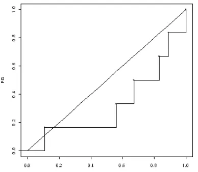
We can produce u-plots for DBMS product pairs in which coincident failures were observed. However, as we saw in Tables 1 and 3, the number of coincident failures observed is very small (≤ 2) for all but one pair (the PG7.0-MS pair on MS faults). We will therefore show only one of the u-plots: for the pair PG7.0-MS on the MS faults. This u-plot is depicted in Fig 2.

The explanation of the u-plot follows: a total of 18 fault reports of MS could be run on the PG7.0 DBMS

product (we’ll call it n); of those 6 caused a coincident failure in PG (we’ll call it r). Since there are 6 coincident failure faults there will be a total of six steps in the u-plot function. The size of each step is 1/r. The

ui values on the x-axis will represent the point i/n, i.e.

the sequence in which the fault was reported in MS. Therefore if the second fault of MS was found to cause a coincident failure in PG7.0 this will be shown as the point 2/18 (i.e. 1/9) on the x-axis. The KS distance for this pair is 0.3889 with the value 0.5041. Since the p-value is so large we do not have enough evidence to reject H0 for this DBMS product pair: we do not have

enough evidence to reject the claim that ui are

uniformly distributed random variables. Therefore on this dataset there is not enough evidence to reject the assumption of constant proportion of common faults.

Fig. 2 - The u-plot computed for the coincident failure causing faults in PG7.0 and MS by the

faults reported for MS.

5.3.2 Tests for equality of proportions. We can also

verify the assumption of constant proportions of coincident failures by partitioning the sample of faults observed and checking whether the proportion of coincident faults differs significantly between the partitions. Initially we have done this by partitioning the samples in two.

(9)

The full details for each pair of DBMS products on each dataset are given in Table 5. The table also contains the results of performing the Fisher’s Exact test and the Binomial proportions test. The Fisher’s Exact test used is the one for 2 X 2 tables. Fisher’s exact test for 2 X 2 tables is used when members of two independent groups can fall into mutually exclusive categories. Quoting from [15]: “The test is used to determine whether the proportions of those falling into each category differ by group.” The Binomial Proportions test (the last column of Table 5 contain the p-values of this test), is only an approximation, whereas the Fisher’s exact test calculates the exact probability. Note that the problem of low sample sizes for coincident faults remains. Whenever possible (i.e. when the number of coincident failures is not 0) we have also tried to calculate the p-values, but we warn the readers that, due to the small sample sizes, these values should be taken with caution. We can see in Table 5 that the p-values for the Fisher’s exact test are not statistically significant at the 5% level. This is due to there being little difference between the two partitions, or in the case of PG7.0-MS on MS faults, the sample size being too small for the p-value to be significant. For this latter pair the p-value is statistically significant at the 10% level (on the MS faults). For the Binomial Proportions test only the p-value of PG-MS on MS faults is statistically significant at the 5% significance level (the p-value is 0.0455); none of the others are significant at the 5% or 10% level.

6. Discussion and Conclusions

Two approaches to predicting the reliability of a 1-out-of-2 FT-node were described in sections 3 and 4. These methods are based on some strong assumptions

about the operational profile and failure rate distributions which may not hold in real operation. Ideally we would like to have detailed information about failure counts and usage time. However vendors discourage users from reporting already known faults and detailed failure data are rarely available even to the software vendors themselves. Also due to the various non-restrictive license agreements of the open-source DBMS products, a DBMS product may be downloaded from a multitude of sources and then installed in many different instances, which makes estimation of the usage time of the DBMS products very difficult. Faced with these difficult problems of data availability, it was necessary to make these strong modeling assumptions in order to make an initial estimate of the potential benefits of fault tolerance with SQL DBMS products.

In section 5.2 we argued that assuming a common failure rate distribution for A-, B- and AB-faults is conservative. Also we have observed in earlier research [4], [3] that AB-faults can fail in different ways in the two DBMS products, and hence can be detected (and potentially corrected [16]). As a result, the estimates that we get using our models for the reliability benefits of diversity will most probably be underestimates: the true benefits may be higher. Despite this conservatism, using the reported faults for the DBMS products in our studies, we would expect an order of magnitude increase in reliability when switching from a single DBMS product to a 1-out-of-2 FT-node. This result should however be treated with caution, due to the small sample sizes and relatively high estimation errors. There also appear to be variations in dependability improvement between different DBMS product pairs.

We used the reported faults from our studies to test for statistical significance of empirical deviation from the “constant proportion of common faults”

Table 5 - Results from performing the Fisher’s exact and Binomial proportions tests on the data sets of the faults study (after the data sets were partitioned into two halves).

DBMS product pair

Faults reported for DBMS

product

1 AB1 2 AB2

Fisher’s exact test Binomial Proportions: Exact probability p-value p-value

IB-PG7.0 IB 14 1 14 0 0.5 0.5 0.309

IB-PG7.0 PG7.0 12 0 12 0 N/A N/A N/A

IB-OR IB 15 0 16 0 N/A N/A N/A

IB-OR OR 2 0 2 0 N/A N/A N/A

IB-MS IB 17 2 18 0 0.2286 0.2286 0.134

IB-MS MS 6 0 6 1 0.5 0.5 0.296

PG7.0-OR PG7.0 15 0 15 0 N/A N/A N/A

PG7.0-OR OR 2 1 2 0 0.5 0.5 0.248

PG7.0-MS PG7.0 16 1 17 1 0.5152 0.7728 0.965

PG7.0-MS MS 9 1 9 5 0.0611 0.0656 0.0455

MS-OR MS 6 0 6 0 N/A N/A N/A

(10)

assumption, using u-plots and two tests for difference between proportions (namely Fisher’s exact and the Binomial Proportions tests). We found that these tests are giving reasonably consistent results with regard to whether the hypothesis of constant proportion of common faults should be rejected. Using these tests at the 90% confidence level, we found, at most, one case out of 12 where the null hypothesis was rejected (and typically 1 in 10 cases might be rejected at the 90% confidence level when the hypothesis is true). This would indicate that the assumption of constant proportions is reasonable for the dataset we used but further work is required to draw more general conclusions due to the small sample size in the dataset.

In summary, for users who want to assess the likely dependability gains achievable if they switch from using a single DBMS product to a 1-out-of-2 diverse server then:

- if the only dependability data available for the DBMS products are the fault reports, and reasonable estimates can be obtained for the failure rate of the DBMS product they are using, then the model described in section 4 can be used to calculate the likely improvements in reliability that they may expect from the changeover to a diverse setup

- if proxies can also be obtained for usage time, then the extended Littlewood model, described in section 3, may also be used to assess the improvements as well as obtain other estimates such as:

- the rate distribution of the common faults - predictions about the expected time to next

diverse server failure etc.

- the two approaches may also be used sequentially to improve the predictions:

- the β values using the proportions approach of section 4 are calculated first, and they are then used to obtain a b parameter for the prior

distribution of the extended Littlewood model Further research is needed to validate the theory presented in this paper. This research includes:

- Methods for obtaining more accurate proxies for usage time.

- Empirical investigations of the predictive performance of the proportions model for actual DBMS product pairs.

- Empirical investigations of the consistency of β factor estimates in successive releases of the same product pair.

- Applying the method to other types of off-the-shelf components (such as diverse web-servers and application servers).

Acknowledgment

This work was supported in part by the U.K. Engineering and Physical Sciences Research Council (EPSRC) via projects DOTS (Diversity with Off-The-Shelf components, grant GR/N23912/01) and DIRC (Interdisciplinary Research Collaboration in Dependability, grant GR/N13999/01) and by the European Union Framework Program 6 via the ReSIST Network of Excellence (Resilience for Survivability in Information Society Technologies, contract IST-4-026764-NOE).

References

1. Popov, P., L. Strigini, S. Riddle, and A. Romanovsky, Protective Wrapping of OTS Components in 4th ICSE Workshop on Component-Based Software Engineering: Component Certification and System Prediction. 2001. Toronto, Canada.

2. Strigini, L., Fault Tolerance Against Design Faults, in

Dependable Computing Systems: Paradigms,

Performance Issues, and Applications, H. Diab and A. Zomaya, Editors. 2005, J. Wiley & Sons, pp: 213-241. 3. Gashi, I., P. Popov, and L. Strigini, Fault tolerance via

diversity for off-the-shelf products: a study with SQL database servers. IEEE Transactions on Dependable and Secure Computing, to appear in the October-December issue, 2007.

4. Gashi, I., P. Popov, and L. Strigini. Fault Diversity Among Off-The-Shelf SQL Database Servers. in Int. Conf. on Dependable Systems and etworks (DS'04). 2004. Florence, Italy: IEEE Computer Society Press,pp: 389-398.

5. Littlewood, B., Stochastic Reliability Growth: a Model for Fault-Removal in Computer Programs and Hardware Designs. IEEE Transactions on Reliability, 1981. R-30(4), pp: 313-320.

6. Lyu, M.R., ed. Handbook of Software Reliability Engineering. 1996, McGraw-Hill and IEEE Computer Society Press.

7. SourceForge, Firebird downloads. 2006, http://sourceforge.net/project/showfiles.php?group_id=90 28.

8. Gray, J. Why Do Computers Stop and What Can be Done About it? in 5th Symposium on Reliability in Distributed Software and Database Systems (SRDSDS-5). 1986. Los Angeles, CA, USA: IEEE Computer Society Press, pp: 3-12.

9. Adams, E.N., Optimizing Preventive Service of Software Products. IBM Journal of Research and Development, 1984. 28(1): pp: 2-14.

(11)

Engineering. 2003. Denver, Colorado, U.S.A, pp: 237-245.

11. Meulen, M.J.P.v.d., L. Strigini, and M.A. Revilla. On the Effectiveness of Run-Time Checks. in Safecomp 2005. 2005. Fredrikstad, Norway: Springer-Verlag, pp: 151-164.

12. Brocklehurst, S. and B. Littlewood, Techniques for prediction analysis and recalibration, in Handbook of Software Reliability Engineering, M.R. Lyu, Editor. 1994, McGraw-Hill and IEEE Computer Society Press. 13. Fisher, R.A., On the interpretation of chi-squared from

contingency tables, and the calculation of P. Journal of the Royal Statistical Society, 1922. 85(1): pp: 87-94. 14. Institute of Phonetic Sciences, Binomial proportions.

2006,

http://www.fon.hum.uva.nl/Service/Statistics/Binomial_p roportions.html.

15. Preacher, K.J., Briggs, N. E., Calculation for Fisher's Exact Test: An interactive calculation tool for Fisher's exact probability test for 2 x 2 tables [Computer software]. 2001, http://www.quantpsy.org.

16. Gashi, I. and P. Popov. Rephrasing Rules for Off-The-Shelf SQL Database Servers. in 6th European Dependable Computing Conf. (EDCC-6). 2006. Coimbra, Portugal: IEEE Computer Society Press, pp: 139-148.

Appendix A –Likelihood equations of the

extended Littlewood model

To produce a general likelihood function for the model discussed in section 3, several different kinds of data need to be considered. For each reported fault we need to consider:

- whether it is present in both DBMS products (i.e. could it have caused a failure in both DBMS products),

- whether it was randomly encountered during testing of one or more DBMS products (i.e. has it been reported in more than one DBMS product). We assume that all three classes of faults (faults that are present in DBMS product A only, B only, or both) have rates independently selected from one common

gamma rate distribution. This produces a 5-parameter model with parameters being three unknown fault-count parameters (say

_A_B

,

_A_B

,

_AB), and two Γ -distributionparameters a, b.

For the data symbols, we will use a convention that observed failure countsn, and also observed timesT of random failure are all, likewise, subscripted to denote which DBMS product(s) contain the faults, and, in addition, superscripted to identify the DBMS product(s) during the testing of which the fault is

randomly encountered. In the case of Ts only, with multiple superscripts (AB or BA), the first of these

superscripts will indicate which DBMS product’s time

T is. For all other cases (whether of subscripts or

superscripts AB) the order has no significance and will be left alphabetic. Finally, parameters lA and lB

represent the testing time for DBMS product A or B respectively. Using these conventions, the extended Likelihood function for the Littlewood model is given by: B ABn B AB A ABn A AB AB AB B AB A AB B AB A