1
IAC-08- C1.3.10
On the Consequences of a Fragmentation Due to a NEO
Mitigation Strategy
J.P. Sanchez
University of Glasgow, Glasgow, United Kingdom, [email protected]
M. Vasile
University of Glasgow, Glasgow, United Kingdom, [email protected]
G. Radice
University of Glasgow, Glasgow, United Kingdom, [email protected]
ABSTRACT
The fragmentation of an Earth threatening asteroid as a result of a hazard mitigation mission is examined in this paper. The minimum required energy for a successful impulsive deflection of a threatening object is computed and compared with the energy required to break-up a small size asteroid. The fragmentation of an asteroid that underwent an impulsive deflection such as a kinetic impact or a nuclear explosion is a very plausible outcome in the light of this work. Thus a model describing the stochastic evolution of the cloud of fragments is described. The stochasticity of the fragmentation is given by a Gaussian probability distribution that describes the initial relative velocities of each fragment of the asteroid, while the size distribution is expressed trough a power law function. The fragmentation model is applied to Apophis as illustrative example. If a barely catastrophic disruption (i.e. the largest fragment is half the size the original asteroid) occurs 10 to 20 years prior to the Earth encounter only a reduction from 50% to 80% of the potential damage is achieve for the Apophis test case.
1. INTRODUCTION
HE threat that asteroids pose to life on Earth has for long been acknowledged [1]. Many techniques to deviate threatening asteroids have been proposed in the last three decades. Some of these techniques propose the application of a very low acceleration on the asteroid, while others use a high speed impact or an explosion to produce an impulsive change in linear momentum. If an impulsive deviation technique is applied to an asteroid, and the energy delivered by the deviation method is above a limit threshold [2; 3], a catastrophic fragmentation, i.e., fragmentation such that the largest fragment contains less than half the mass of the original asteroid, is likely to occur.
2
completely fracture the asteroid. As will be shown inthe paper, for some warning times the collision energy required for an impulsive deviation technique can rise well above the theoretical catastrophic fragmentation limit. As a consequence the asteroid can fragment in an unpredictable number of pieces having different mass and velocity. The velocity associated to each piece of the asteroid uniquely determines its future trajectory.
In the paper, we consider two possible cases: the fragmentation being the desired outcome of the deviation strategy or the undesired product of a mitigation mission. In the latter case we will analyse the evolution of the cloud of fragments and the probability that the bigger pieces in the cloud has to impact the Earth. In the former case, we will investigate some possible strategies that allow us to minimize the risk of impact from the bigger pieces in the cloud.
Fragmentation is here considered as a stochastic process, using a different probability distribution to describe both fragment size and velocity distribution. The evolution in time of the cloud of fragments is computed by evoking Liouville’s theorem for Hamiltonian systems and considering two body dynamics. The analysis of the dispersion of fragments and consequences of the fragmentation are applied to asteroid Apophis as illustrative example.
2. FRAGMENTATION OF ASTEROIDS
First, the asteroid resistance to fragmentation will need to be estimated in order to assess the likelihood of a fragmentation outcome from an impulsive mitigation technique. The critical specific energy Q* is defined as the energy per unit of mass necessary to barely catastrophically disrupt an asteroid [3]; an asteroid is barely catastrophically disrupted when the mass of the largest fragment of the asteroid is half the mass of the original asteroid, or in other words, the remaining mass of the original asteroid is half the initial mass. If
f
r is the fragmentation ratio, defined as:max
r
a
m
f
M
=
, (1.1)where mmax is the mass of the largest fragment and Ma
the initial mass of the asteroid, then a catastrophic fragmentation is defined as a fragmentation where
0.5
r f < .
This paper is addressing the issue of fragmentation of small to medium size asteroids. These are celestial objects ranging from 40m to 1km in diameter, which constitute the main bulk of the impact threat. Small objects in this range rely only on their material strength properties to avoid break up, while for large objects gravity plays a fundamental role. Asteroids smaller than 40m in diameter are expected to dissipate at a high altitude in the Earth atmosphere (2), thus nothing smaller than 40m will be included in this analysis. On the other hand, the survey of large objects, hence those above 1km diameter, is believed to be almost complete,
therefore only the remaining small not discovered asteroids pose a threat [10].
The uncertainty associated to the description of the fragmentation process is clear if one looks at the
different scaling laws in the literature [11].
Furthermore, the exact value of Q* depends on a
number of factors, such as the composition and structure of the asteroid or the velocity and the size of the impactor. For the sake of the analysis in this paper, a complete and exact description of the fragmentation process is not required and an approximate estimate of
the value of the critical specific energy Q* is sufficient.
The work of Ryan and Melosh [3] and Holsapple[12]
provided the necessary tools to understand and approximate the qualitative limits of the critical specific energy Q* for the range of studied asteroids.
Fig. 1 shows the critical specific energy Q* for
asteroids ranging from 40m to 1km diameter, computed by using the scaling laws provided by Ryan
and Melosh [3] and Holsapple[12].
100 200 300 400 500 600 700 800 900 1000 101
102 103 104
Asteroid Diameter, m
C
ri
ti
ca
l
S
p
ec
if
ic
E
n
er
g
y
Q
*,
j/
k
g
Ryan & Melosh Basalt for a 10 km/s impact Ryan & Melosh Strong Mortar for a 10 km/s impact Ryan & Melosh Weak Mortar for a 10 km/s impact Ryan & Melosh Basalt for a 50 km/s impact Ryan & Melosh Strong Mortar for a 50 km/s impact Ryan & Melosh Weak Mortar for a 50 km/s impact Holsapple Scaling Law
100 j/kg 1000 j/kg
Fig. 1: Critical Specific Energy Q* to barely catastrophically disrupt an asteroids with a diameter ranging from 40m to 1km using Ryan and Melosh
[3] and Holsapple[12]. Ryan and Melosh [3] work
provide a scaling law that takes into account both velocity of the impactor and impacted object
diameter, while Holsapple[12]’s scaling law is only
function of the impacted object diameter.
In the light of the results shown in Fig. 1, two general qualitative limits were considered: one at 1000 j/kg and a second at 100 j/kg. The 1000 j/kg limit can be interpreted as an almost certain catastrophic
fragmentation, since the specific energy Q* foreseen
by the scaling laws in Fig. 1 is almost always below the 1000 j/kg limit, and even for some cases this limit is more than one order of magnitude above the predicted
Q*. Instead, the 100 j/kg is at the same energy level of
most of the Critical Energies predicted by Fig. 1, and more importantly, the 100 j/kg limit is, in general, above the four predicted Q* using Ryan and
Melosh[3]’s Mortar strength. If asteroids have the
[image:2.595.316.544.297.469.2]3
considered as a reasonable fragmentation limit
according the results of Ryan and Melosh [3] and
Holsapple [12] scaling laws.
3. NEO DEFLECTION REQUIREMENTS
In order to compute the minimum deflection required to deviate a threatening asteroid, we will need to define the minimum distance that an asteroid needs to be shifted in order to miss the Earth. We consider
one Earth radius
R
⊕ as the minimum required deviationdistance and we take into account the gravitational pull of the Earth during the asteroid final close approach by using the following factor:
2
2
1
a e
p p
r
r
r v
µ
ε
∞
=
=
+
(2.1)where ra is the minimum distance between the
hyperbola asymptote and the Earth, rp is the perigee
distance, which is R⊕in our case, µe is the
gravitational constant of the Earth and v∞ the
hyperbolic excess velocity. Note that the correcting factor will only depend on the hyperbolic excess velocity of the threatening object.
Table 1 summarizes the orbital characteristics of the test case that will be used in the subsequent
analysis. Apophis is an interesting test case not only
because is the most renowned asteroid among those posing a noticeable threat to Earth, but also because if another threat to Earth is to be appear, it will probably
have orbital elements not too far from those of Apophis
[14].
Apophis
Semimajor axis a, km 0.922
Eccentricity e 0.191
Inclination i, deg 3.331
Ascending node Ω, deg 204.5
Pericenter angle ω, deg 126.4
Mean anomaly M, deg 222.3
Epoch, MJD 53800.5
tMOID, MJD 62240.3
Hyperbolic factor
ε
2.16Impact velocity, km/s 12.62
Mass Ma, kg 2.7x10¹⁰kg
Table 1: Apophis summary of orbital characteristics
and mass. tMOID stands for time at Minimum Orbital
Interception Distance, and it is used here as equivalent to the time of the hypothetic impact.
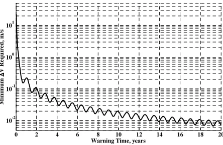
3.1. Minimum Change of Velocity
Once the minimum distance to avoid collision is set, the minimum change of velocity to provide a safe deflection can be calculated. Fig. 2 presents the
necessary change of velocity to deviate Apophis by a
distance of 2.16×R⊕ if the change is applied within an
interval of time spanning 20 years before the
hypothetical impact at time tMOID. The minimum
change of velocity required to deviate an object by a given distance was computed by means of proximal motion equations expressed as a function of the variation of the orbital elements, the variation of the orbital elements was computed then with Gauss’
planetary equations [15].
0 2 4 6 8 10 12 14 16 18 20
10-2 10-1 100 101
Warning Time, years
M
in
im
u
m
∆∆∆∆
V
R
eq
u
ir
ed
,
m
/s
Fig. 2: Minimum Change of velocity to deviate
Apophis by a distance 2.16xR⊕as a function of
warning time. Warning time is referred here as the time available to correct the trajectory of a threatening object, thus the time difference between the instant at which the change of velocity takes place and the time of the hypothetic impact.
3.2. Kinetic Impactors and Nuclear Interceptors
Only impulsive mitigation actions could provide specific energies of the order of the Critical Energy Q* from Fig. 1. Hence, deflection strategies such as kinetic impactor and nuclear interceptor could possibly originate a catastrophic outcome as a result of a deviation attempt. The remaining of this section will briefly describe the main features of these two mitigations strategies, more comprehensive description
can be found in other work by the authors [8].
The Kinetic Impactor is the simplest concept for asteroid hazard mitigation: the asteroid linear momentum is modified by ramming a mass into it. The impact is modelled as an inelastic collision resulting into a change in the velocity of the asteroid multiplied
by a momentum enhancement factor [16]. This
enhancement is due to the blast of material expelled during the impact, although if the asteroid undergoes a fragmentation process after the kinetic impactor has rammed into it, the enhancement factor should be considered 1. Accordingly, the variation of the velocity of the asteroid due to the impact is given by:
(
)
/
/ /
s c
a s c
a s c
m
M
m
β
∆
=
∆
+
v
v
, (2.2)where β is the momentum enhancement factor, ms c/ is
the mass of the kinetic impactor, Mais the mass of the
asteroid and
∆
v
s c/ is the relative velocity of thespacecraft with respect to the asteroid at the time when the mitigation attempt takes place.
[image:3.595.317.539.137.282.2]4
compute the Specific Kinetic Energy (SKE) that an asteroid would have to absorb from a kinetic impactor attempting to modify the asteroid trajectory:
(
)
22
/ 2
/ /
2
/
1 1
2 2
a s c
s c s c
a
a a s c
M m
m v
SKE v
M β M m
+ ∆
= = ∆
⋅ ⋅ (2.3)
The Nuclear Interceptor strategy, instead, assumes a spacecraft carrying a nuclear warhead and intercepting with the asteroid. The model used in this
study, fully described in Sanchez et al. [8], is based on
a stand-off configuration over a spherical asteroid, i.e., the nuclear device detonates at a given distance from the asteroid surface. The energy released during a nuclear explosion is carried mainly by X-rays, neutrons and gamma radiation that are absorbed by the asteroid surface. This sudden irradiation of the asteroid, which causes material ablation and a large and sudden increase of the surface temperature, would induce a stress wave that while propagating through asteroid could trigger not only the surface material ablation that was intended to obtain a change of velocity, but also the fragmentation of the whole body. The Specific absorbed Nuclear Energy (SNE) is defined here as the portion of the energy release that is radiated over the asteroid divided by the mass of the asteroid.
0 2 4 6 8 10 12 14 16 18 20
102 104 106 108
S
p
ec
if
ic
M
it
ig
a
ti
o
n
E
n
er
g
y
,
j/
k
g
0 2 4 6 8 10 12 14 16 18 2010
0
101 102
0 2 4 6 8 10 12 14 16 18 2010
0
101 102
Warning Time, years
Im
p
a
ct
V
el
o
ci
ty
,
k
m
/s
Vrel for ms/c=25e3kg Vrel for ms/c=5e3kg
SKE ms/c=5e3kg SKE ms/c=25e3kg 1000 j/kg 100 j/kg SNE
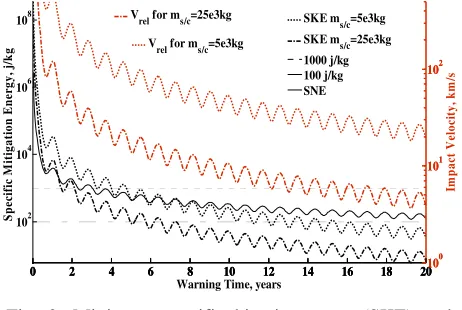
Fig. 3: Minimum specific kinetic energy (SKE) and specific absorbed nuclear energy (SNE) for a mitigation mission at a variable warning time (left Y axis). Relative impact velocities for two kinetic
impactors (right Y axis), ms/c=5000kg and
ms/c=25000kg. The enhancement factor is assumed
2 as a conservative value for this computation [8].
Fig. 3 presents the SKE and SNE as a function of warning time that kinetic impactor and nuclear interceptor, respectively, should provide given the delta-velocities required by Fig. 2. The two aforementioned fragmentation limits of 1000 j/kg and 100 j/kg are also superposed in the figure. The impact velocities for two possible impactors, ms/c=5000kg and ms/c=25000kg, are plotted as well with the right Y axis of Fig. 3. It should be noted that a Kinetic Impactor with ms/c=5000kg would need more than 100 km/s to deliver a collisional energy of 1000 j/kg or higher, which even taking into account retrograde impact trajectories does not seem possible with current technology. On the other hand, the two kinetic impactors used as example achieve energy values that
could possibly trigger a fragmentation with relative velocities lower than 50km/s, which can be achieve
using retrograde orbits [17; 18].
The two suggested limits (1000 j/kg and 100 j/kg) must be taken cautiously when assessing the likelihood of fragmentation triggered by a nuclear interceptor. Since these two suggested limits were estimated from
hypervelocity impact studies [19], the actual
fragmentation energies for an asteroid being deflected by a nuclear device may be different, because of the different physical interaction. However, in this work we considered that the shock wave caused by an impact and the thermal stress wave generated by the nuclear explosion are analogous, and therefore the associated fragmentation energies are expected to have similar order of magnitude.
4. STATISTICAL MODEL OF A
FRAGMENTED ASTEROID
As it can be concluded from the energetic requirements of a hazard mitigation mission, the risk of an undesired break-up of an asteroid during a
deflection attempt cannot be ignored. The
consequences of an undesired fragmentation can be evaluated by studying the evolution of the cloud of fragments generated during the break-up process. Instead of building a dynamical model of the fragmentation process, in this section we propose a statistical model of the initial distribution of the fragments with associated positions and velocities.
4.1. Fragmented Asteroid Dispersion
The position and velocity of every piece of a fragmented asteroid can be described as a stochastic process, even if the dynamical system is deterministic, since the initial conditions of the system are not known and they can only be assessed through a probability density function. Considering a scalar function describing the probability density of a dynamic system such as ρ
(
X( )t)
=ρ( , ; )x v t , where ρ( , ; )x vt is theprobability of a fragment to have position x and
velocity v at a time t. The probability density function
(
( )t)
ρ X relates to an initial probability density
function ρ
(
X(0))
through:(
( ))
(
( ) t( (0)))
(
(0))
( )
0t t d
ρ δ φ ρ
Γ
=
∫
− ΞX X X X (3.1)
where t( (0))
φ X denotes the flux of the system, or
evolution of the state X(0)=[ (0), (0)]x v T over a time-span t so that φt( (0))X =[ ( ), ( )]xt vt T, ( )δ y is a multi-dimensional Dirac-delta, which represents the product of the one-dimensional Dirac-delta functions, that will allow a probability ρ
(
X(0))
to be added to the total probability of ρ(
X( )t)
, only if the initial state vector(0)
X can effectively evolve to X( )t , and finally,
( )
0dΞ refers to the product of the one-dimensional
[image:4.595.54.285.356.511.2]5
x y zdx dy dz dv
⋅
⋅
⋅⋅
dv⋅
dv , and defines the volume of aninfinitesimal portion of the phase space Γ, which is
the feasible phase space where the system evolves.
If we introduce the new variable t( (0))
φ =
z X and
the associated Jacobian determinant as ( (0))
(0) t φ ∂ = ∂ X J X ,
we can substitute the differential dΞ
( )
0 by dζ J inEq.(3.1), where dζ is the product of the
one-dimensional differentials components of the vector z
and J is the absolute value of the Jacobian
determinant. This allows us to integrate using the
phase space at time t and Eq.(3.1) results in the
following integration:
(
( ))
(
( ))
(
t( ); 0)
dt t ζ
ρ δ ρ φ−
Γ
=
∫
−X X z z
J (3.2)
From the Liouville’s theorem, which states that for a Hamiltonian system the density of states in the phase
space remains constant with time [20], we know that
1 =
J , thus Eq.(3.2) can be solved giving:
(
( ))
( t( , ); 0)t
ρ X =ρ φ− x v
(3.3) Eq. (3.3) implies that the probability that a particular
fragment has position xand velocity vat a time t is the
same probability of having the initial conditions that can make the fragment dynamically evolve to the particular state X( )t .
If we now compute the state transition matrix
0
( , )t t
Φ : 0 0 0 0 0 ( ) ( ) ( ) ( ) ( , ) ( ) ( ) ( ) ( ) t t t t t t t t t t ∂ ∂ ∂ ∂ = ∂ ∂ ∂ ∂ x x x v Φ v v x v
, (3.4)
we can directly map the initial state vector X( )t0 to
the final state vector X( )t , which is necessary to
calculate Eq.(3.3): 0 0 0 ( ) ( ) ( ) ( , ) ( ) t t
t t t t
= x x
v Φ v (3.5)
Since we are interested in studying the dispersion of a cloud of particles, we can work in relative coordinates to study the differences in position and velocity with respect the unperturbed orbit of the asteroid prior to fragmentation. Eq.(3.5) can be simplified by assuming that all the fragmented particles depart from the centre of mass of the asteroid (i.e., the relative initial position ∆x( )t0 is 0), and by computing
only the relative final position ∆x( )t : 0 0 ( ) ( ) ( ) ( ) t t t t ∂ = ∂ x x v v (3.6)
This simplifies the problem considerably since only the 3 3× transition matrix ∂x( )t ∂v( )t0 is required. The
transition matrix is given by the product of the linear proximal motion equations and the Gauss’ planetary equations (for further details see Vasile and Colombo
[15]). This calculation provides a linear approximation
of the nonlinear two body dynamics, but if the dispersive velocity is small compared to the nominal
velocity of the unfragmented asteroid, it is a workable
approximation [15].
Since we are interested in the probability to find a fragment in a certain position in space at a particular time t, the probability function ρ( , ; )x vt will need to be integrated over all the feasible space of velocities:
( ; ) ( , ; ) ( ) ( t( , );0) ( )
P t ρ t dυ t ρ φ− dυ t
Γ Γ
=
∫
=∫
x x v x v (3.7)
where dυ( )t is the product of the one-dimensional
differentials components of the velocity, dvx⋅dvy⋅dvz.
Since the probability density function ρ( , ; 0)x v is
the probability to have a fragment in a position x(0)
with velocity v(0) and we already assumed that the
dispersion of fragments initiates from the centre of mass of the unfragmented asteroid, then we can express
( , ; 0)
ρ x v as the product of two separated probability
density function:
( , ; 0) ( (0) ) G( (0))
ρ x v =δ x −r0 ⋅ v (3.8)
where δ( (0)x −r0) is giving the probability of a
particular fragment to have position x(0)−r0, where
0
r is the position of the centre of mass of the
unfragmented asteroid at t=0, and G( (0))v is
associating the probability to have velocity v(0) to the
same fragment. Now, Eq.(3.7) can be rewritten using Eq.(3.8) as:
( ; ) ( t( , ) ) ( t( , ) ) ( )
P t δ φ− Gφ− dυ t Γ
=
∫
x− 0 ⋅ vx x v r x v (3.9)
where t( , )
φ−
x
x v and t( , )
φ−
v
x v are the components of
the position and velocity respectively of the flux
( , ) t
φ−
x v . Now, similar to what it was done with
Eq.(3.1), the element of volume of the space of
velocities dυ( )t can be related to the element
(0)
dξ =dx dy dz⋅ ⋅ through their Jacobian: ( )
( ) (0)
(0)
t
dυ t = ∂ dξ
∂
v
x (3.10)
allowing us to solve the integral in Eq.(3.7):
* ( ) ( ; ) (( ( , ) ) (0) t t
P t = ∂ G φ−
∂ v
v
x x v
x (3.11)
where
v
* is the solution of the equation:* ( , )
t
φ− =
x 0
x v r (3.12)
so that the ( t( , ) )
δ φ−
− 0
x
x v r is 1. Besides, the absolute
value of the Jacobian in Eq.(3.11) relates to the transition Matrix [∂x( )t ∂v( )t0 ] in Eq.(3.6) as follows:
0
( ) 1 1
(0) (0) ( )
( ) ( ) t t t t ∂ = = ∂ ∂ ∂ ∂ ∂ v
x x x
v v
(3.13)
6
10 0
1 ( )
( ; ) ( )
( ) ( )
( )
t
P t G t
t t t − ∂ = ∂ ∂ ∂ x x x v x v (3.14)
4.2. Velocity Dispersion Model
We have assumed, in Eq.(3.8), that the probability density function depends on two terms, a Dirac delta such as δ( (0)x −r0)for the position, which is equivalent to one Dirac delta function for each one of the components of the vector x(0), and a function G( (0))v
that describes the dispersion of the values of the initial velocity v(0). For the latter purpose, we will use three Gaussian distribution; each Gaussian distribution will describe the velocity dispersion in one direction of the Hill’s reference frame tˆ− −nˆ hˆ(or tangential, normal and out-of-plane direction):
(
)
( ) ( ) ( ) 2 2 2 2 2 2 2 2 2(0), (0), (0) 1 2
1 1
2 2
t t t
n n h h
n h
t n h
v
t
v v
n h
G v v v e
e e µ σ µ µ σ σ σ π
σ π σ π
− −
− − − −
=
⋅ ⋅
(3.15)
Six parameters will be needed in order to define the dispersion of velocities: three mean velocities
[
µt µn µh]
= , and three standard deviations
[
σt σn σh]
=
σ .
Assuming a kinetic impactor scenario, we can think that, at an infinitesimal instant after the impact, but before the fragmentation takes place, the system asteroid-spacecraft form a single object, which moves according to the law of conservation of linear momentum. In fact, after the kinetic impactor mission triggers a catastrophic fragmentation, it is reasonable to think that the system asteroid-spacecraft would preserve the total linear momentum. Hence, given the SKE of a particular collision, Eq.(2.3) will provide the change of velocity of the centre of mass of the system only by considering the momentum enhancement factor β equal 1. It seems also sensible to think of the mean vector =
[
µt µn µh]
as the change of velocity of the centre of mass, since the highest probability to find a fragment should be at the centre of mass of the system. As a result, the norm of the mean of the dispersion should be:(
)
/
/
2 a s c
a s c M m SKE
M m
= ∆ =
+ a
v (3.16)
The direction of is defined by the direction of
the vector ∆vs c/ . Since the trajectory of kinetic
impactor should be designed to achieve the maximum
possible deviation, should be directed along the
tangential direction [15]. Accordingly, given the SKE
of the collision, the mean velocity dispersion vector can be taken as:
(
)
/ / 2
0 0
a s c
a s c
M m SKE
M m = + (3.17) Just as it is sensible to think that after a dish has shattered on the floor, the smallest fragments are always found the furthest, one would expect that the smaller the fragments of the asteroid are the larger will be their velocity dispersion σ=
[
σt σn σh]
, hence the mass of the fragment must have an influence on the dispersion of velocities. Let us assume that a fragment with mass mi has a velocity ∆vi defined by an inelasticcollision such that (note that in the following, it is considered that ms/c is always orders of magnitude
smaller than both Ma and mi, thus Ma+ms c/ ≈Ma and
/
s c
i i
m +m ≈m ):
/ i
i i s c SKE m
m v∆ ≈m ∆v ⋅ (3.18)
where i
SKE m
v
⋅
∆ is a collisional velocity such that the fragment mi takes with it its share of collisional energy
SKE, that is:
/ 2 i i SKE m s c SKE m v m ⋅ ⋅ ⋅
∆ = (3.19)
Clearly,
i
SKE m
v
⋅
∆ is only a mathematical entity that
helps us to develop the hypothesis at hand, the real impact occurs between the unfragmented asteroid with
mass Ma and the spacecraft with mass ms/c at a relative
velocity of:
(
)
/ 2 /
s c a s c
v SKE M m
∆ = ⋅ ⋅ (3.20)
Writing Eq.(3.19) as a function of the real impact
velocity ∆vs c/ of the spacecraft, Eq.(3.20), leads us to:
/ i
i
SKE m s c
a
m
v
v
M
⋅
∆
=
⋅ ∆
(3.21)Using the virtual inelastic collision Eq.(3.18) and Eq.(3.21), we can write ∆vi as:
/
/
s c i
i s c
i a
m m
v v
m M
∆ = ⋅ ∆ (3.22)
As it has been said before, the centre of mass of the cloud of fragments is likely to follow the law of
conservation of linear momentum (i.e.,
/ /
a a s c s c
M ∆v ≈m ∆v ), hence Eq.(3.22) finally settles
down to the following expression:
a i a i M v v m
∆ = ⋅ ∆ (3.23)
Note that Eq.(3.23) is only one step away from: 1
2 x
m v∆ =constant (3.24)
when x is equal to 2. Hence, we are assuming a
7
Eq.(3.24)) to their fragment size and velocity
experimental data; Gaultet al. [21] found an exponent
of 2.25 for his cratering experiments, while Davis and
Ryan[19]found exponents between 1.92 and 1.41 on
their fragmentation experiments. An equipartition
effect was also suggested by Wiesel [22] while
studying the explosion of objects such as spacecrafts in Earth orbit.
Recalling the definition of standard deviation,
2 2
σ = v − v , and assuming v
=
0
for ahomogeneous spherical dispersion from the centre of mass of the cloud of fragments, we can compute the
norm of the standard deviation of the velocities σ
( )
miusing Eq.(3.23) as:
0
( i)
i
a
M m
m
σ = ⋅σ (3.25)
where σ0 is now:
0 a v
k
σ = ∆ (3.26)
with k a constant value. The constant k is 1 if we
consider the velocity of the fragment with mass mi as described above, i.e., Eq.(3.23).
In fact, one could think of k as the efficiency of transmission of the collisional energy. If part of the collisional energy is lost in processes such as melting
or breaking, one could expect k to be larger than 1, on
the other hand, k could also be smaller than 1 for
fragments coming from areas in the asteroid where there was higher reservoir of collisional energy, e.g., close to the impact site. Therefore, it would be sensible
to expect that small fragments may have k equal to 1 or
smaller, since small fragments must come from areas with a higher reservoir of collisional energy so that this energy was able to break the material to smaller pieces.
Large fragments may have instead k larger than 1 from
opposite reasons. Using the experimental data
published by Davis and Ryan [19], one can fit their
experiments with velocity dispersion data available to
find an average value of k. Doing so, k results 1.4.
Thus,
0
1.4
a v
σ =∆ (3.27)
To finish, the norm of standard deviation of velocity is σ
( )
mi as in the Eq.(3.25), and since weassume an homogeneous spherical dispersion on the initial velocities at the break-up point, we can write the vector of the standard deviation as assuming three equal 1-dimensional values:
0 0 0
1 1 1
3 i 3 i 3 i
a a a
M M M
m σ m σ m σ
= ⋅ ⋅ ⋅
σ (3.28)
5. EVOLUTION OF THE CLOUD OF
FRAGMENTS
The following six figures, Fig. 4 to Fig. 9, show the evolution of the probability density function of a fragmentation occurring after providing 500 j/kg of
collisional energy to Apophis (test case in Table 1).
Such a kinetic impact would provide an approximate
change of velocity of ∆va =0.02m s by using an
impactor with mass ms c/ of 10,000kg. The figures are
showing the volume enclosing 97% chances to find
each single 1010kg-fragment at different times or
different true angles. Break-up is set to occur at the pericentre of the unperturbed orbit, and the sequence of
figures show the 97% volume at true anomalies of 450,
[image:7.595.348.522.375.507.2]900, 1800, 2700, 3150 and 3600.
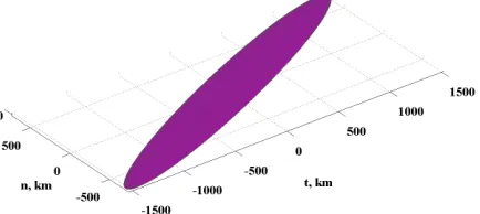
Fig. 4: ∼97% probability volume for a fragment with
[image:7.595.323.540.563.660.2]mass 1010kg at true anomaly of 450.
Fig. 5: ∼97% probability volume for a fragment with
mass 1010kg at true anomaly of 900.
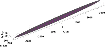
Fig. 6: ∼97% probability volume for a fragment with
8
Fig. 7: ∼97% probability volume for a fragment with
mass 1010kg at true anomaly of 2700.
Fig. 8: ∼97% probability volume for a fragment with
mass 1010kg at true anomaly of 3150.
Fig. 9: ∼97% probability volume for a fragment with
mass 1010kg at true anomaly of 3600.
The volumes plotted in Fig. 4 to Fig. 9 can be also understood as the physical shape of the cloud of fragments of a certain size, since the probability density function is describing the regions where, statistically at least, there is a higher density of particles. The most prominent feature that stands out from the images above is the ellipsoidal shape of volume enclosing a particular probability, or cloud of particles. In order to better understand the dynamics of the dispersive cloud of particles, we can try to understand the evolution of the four salient features of the elliptical cloud. These four features are: the
semimajor axis a, the semiminor axis b, the dispersion
along the h axis or out-of-plane and the angle
α between the semimajor axis a and the tangential
direction axis t.
Fig. 10: schematic of the 4 features describing the shape and attitude of the elliptic shaped cloud of fragments.
Fig. 11 summarizes the evolution of the four aforementioned features that describe the volume enclosing 97% probability to find each one of the
existing fragments with mass of 1010kg. Larger
fragments will have smaller volumes, but the same
shape, since their velocity dispersion σ will be smaller
by a factor of
1 10 10
10
10
kg m kg
> × , while the opposite
occurs for smaller objects. Fig. 11 extents also the evolution shown in Fig. 4 to Fig. 9 to complete a two years propagation from the break-up point.
0 0.2 0.4 0.6 0.8 1 1.2 1.4 1.6 1.8 2 0
2000 4000 6000 8000 10000
Time, years
L
en
g
th
,
k
m
0 0.2 0.4 0.6 0.8 1 1.2 1.4 1.6 1.8 20 20 40 60 80 100
A
n
g
le
,
d
eg
re
es
Semimajor axis a Semiminor axis b Out-of-plane h
α αα α
Fig. 11: Two years evolution of the four salient features defining the elliptical cloud enclosing 97%
probability to find each fragment of 1010kg.
It is important to note that the evolution of the shape of the cloud is essentially driven by the dynamics of the system, thus the proximal motion equations that we used to define the transition matrix in Eq.(3.6). For example, among the three parameters defining the size
of the ellipse, the semimajor axis a is the only
parameter that is unbounded, much like the change of velocity in tangential direction, which causes an unbounded drift from the unperturbed initial orbit.
6. CONSEQUENCES OF A FRAGMENTATION
If the impact with Apophis is assumed to occur at the MOID point, then, the impact likelihood can be calculated by integrating over the volume inside a
sphere centred at the Apophis’ MOID point with radius
equal to the Earth capture volume dV r( ):
ˆ
h
ˆ
b
ˆ
t
ˆ
n
ˆ
a
[image:8.595.318.530.62.186.2] [image:8.595.60.276.200.295.2] [image:8.595.313.542.398.537.2]9
( )
0
( 0)
)
( ;(
)
( )
V r R
MOID V r
L
P
t
t
dV r
ε ⊕
= ⋅
=
−
=
∫
x
⋅
(5.1)Note that the capture volume is approximated by the Earth radius corrected with the aforementioned
hyperbolic factor
ε
, to account for the gravitationalfocusing of the Earth.
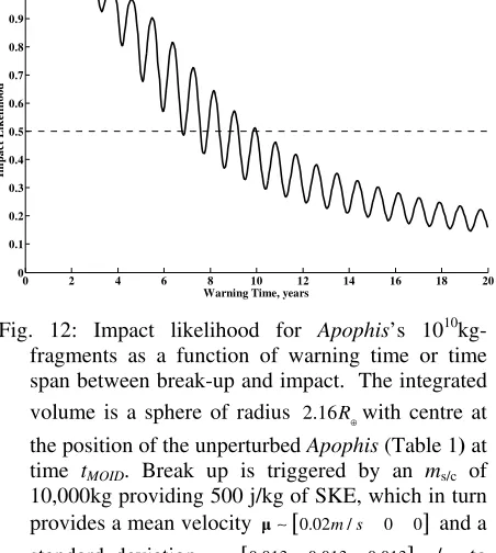
From Eq.(5.1) we can see that the total impact likelihood for a particular fragment size is only a function of the time of the closest approach tMOID (see Table 1), the time at which the break up occurred (the difference between these two times is here referred to as the warning time) and the specific collisional energy used to break up the asteroid. Fig. 12 shows the evolution along warning time of the impact likelihood
for 1010kg-fragments emanating from a hypothetical
fragmentation of Apophis.
0 2 4 6 8 10 12 14 16 18 20
0 0.1 0.2 0.3 0.4 0.5 0.6 0.7 0.8 0.9 1
Warning Time, years
Im
p
a
c
t
L
ik
el
ih
o
o
d
Fig. 12: Impact likelihood for Apophis’s 1010
kg-fragments as a function of warning time or time span between break-up and impact. The integrated volume is a sphere of radius 2.16R⊕with centre at
the position of the unperturbed Apophis (Table 1) at
time tMOID. Break up is triggered by an ms/c of 10,000kg providing 500 j/kg of SKE, which in turn
provides a mean velocity ∼
[
0.02m s/ 0 0]
and astandard deviation σ∼
[
0.013 0.013 0.013]
m s/ tothe 1010kg-fragments.
An important difference of the calculation in Fig. 12 with respect the calculations in Fig. 4 to Fig. 9 is the fact that for Fig. 12 the break up of the asteroid is moving backwards in time, in order to have an increase in warning time, while the hypothetical impact time
tMOID is kept fixed. A consequence of this is that the
break up occurs at different orbital positions of the
unperturbed orbit of Apophis, and the periodic
variations of the impact likelihood that can be observed in Fig. 12 are in fact due to this change of the orbital position of the break up point. The periodic minimum occurs at each orbit when the break up is at the pericentre of the orbit, and the maximum occurs at the apocentre. This is not surprising, since, for a fixed
change of velocity δv of a fragment, the maximum
change of orbital period occurs when the orbital velocity is maximum, which happens at the pericentre, therefore the maximum dispersion of fragments
happens also when the break up point is at the pericentre.
6.1. Fragment size distribution
It is out of the scope of this paper to describe the physics of the fragmentation of a brittle solid, such as an asteroid, and a simple statistical distribution of fragments will serve better to our purposes, which are to discern the intrinsic risks of the asteroid hazard mitigation.
Early works in collisional fragmentation already used accumulative power law distribution to model
fragment size distribution [23]. Two- or three-
segments power laws had been found to fit much better
to experimental data [19; 24], specially when the
fragmentation data comprises sizes many orders of magnitude smaller than the original size. However, for the analysis carried out here we will use only one segment accumulative power law distribution such as:
(
)
bN
>
m
=
Cm
− (5.2)since this is already an acceptable approximation for a qualitative analysis of a range of 3 orders of magnitude in mass. In Eq.(5.2), if mmax is the mass of the largest
fragment, N(≥mmax) must be 1, therefore the constant
C must be:
max
b
C
=
m
(5.3)Now, If we integrate the mass over all the particles, the total mass must be equal to the unfragmented
asteroid mass Ma:
(
)
max
0
1 max
1
b a
M
bC
M m dN m
b
−
= ⋅ =
−
∫
(5.4)Using Eq.(5.3) in Eq.(5.4), the exponent b becomes
a function only of the ratio between the largest fragment mass mmax and the total mass of the asteroid
Ma:
1 max
1 a
m b
M
−
= +
(5.5)
where the fraction mmax Mais fragmentation ratio fr.
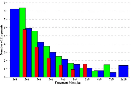
Fig. 13 shows the number of fragments of different sizes expected for three catastrophic fragmentations using a power law distribution such as Eq.(5.2):
0.5 r
f = (blue bars), fr =0.25(green bars) and
0.1 r
f = (red bars). Only the range of fragments that
[image:9.595.58.284.261.513.2]10
1e10 7e9 4e9 2e9 1e9 9e8 5e8 3e8 2e8 1e8 0 1 2 3 4 5 6 7 8 9
Fragment Mass, kg
N
u
m
b
er
o
f
F
ra
g
m
en
[image:10.595.56.285.55.205.2]ts
Fig. 13: Approximated number of pieces expected to be found in a fragmentation cloud of an asteroid with
2.7x10¹⁰kg of mass resulting from disruptions with
fr=0.5 (blue bars), fr=0.25 (green bars) and fr=0.1 (red bars). The largest fragment, i.e., surviving mass of the asteroid, is counted in the initial bin of the histogram for each level of disruption.
6.2. Average Predicted Impacts
Here we present the impact likelihood over a time span of 20 years. Five different size samples were
computed: 1010kg, 109kg, 5x10⁹kg,, 108kg and
5x10⁸kg. By definition, from a fragmentation with
fr=0.5, we have at least a large fragment with half the
mass of the original asteroid, 1.35x10¹⁰kg, the
remaining pieces of the asteroid are assumed to follow the power law distribution such as Eq.(5.2), and their impact likelihoods approximated to the closest of the calculated masses. Table 2 summarizes the computed fragment groups and the average number of fragments belonging to each group.
Bins N(fr=0.5) Mass
10 9
1.35 10x kg≥m>7 10x kg 2 10
1 10x kg
9 9
7 10x kg≥m>2 10x kg 2 9
5 10x kg
9 8
2 10x kg≥m>7 10x kg 4 9
1 10x kg
8 8
7 10x kg≥m>2 10x kg 8 8
5 10x kg
8 7
2 10x kg≥m>9 10x kg 13 8
[image:10.595.315.543.59.244.2]1 10x kg
Table 2: Fragment groups used for the computation of impact likelihood and average number of impacts for a barely catastrophic fragmentation. Note that
the smallest mass is 9x10⁷kg, since the lower limit
is set by the lower diameter limit of 40m.
0 2 4 6 8 10 12 14 16 18 20
0 0.1 0.2 0.3 0.4 0.5 0.6 0.7 0.8 0.9 1
Warning Time, years
Im
p
a
ct
L
ik
el
ih
o
o
d
1010kg 5x10⁹kg 109kg 5x10⁸kg 108kg
Fig. 14: Impact likelihood evolutions of the 5 fragments size computed.
0 2 4 6 8 10 12 14 16 18 20
0 5 10 15 20 25 30
Warning Time, years
A
v
er
a
g
e
Im
p
a
ct
1010kg 5x10⁹kg 109kg 5x10⁸kg 108kg Total
Fig. 15: Average number of impacts for each fragment size group.
Fig. 14 and Fig. 15 show the evolution with warning time of the individual impact likelihood for each fragment size and the number of impacts that should be expected for each fragment size, which is simply the result of the number of fragments multiplied by the impact likelihood. As was expected, the smaller a fragment is the lower its impact likelihood, which is due to the higher velocity dispersion. Despite that, the number of expected impacts grows with a decreasing mass of the fragments and even if the break-up occurred 20 years in advance still a few impacts should be expected.
6.3. Expected Damage
As shown in Fig. 15 from last section, if an asteroid hazard mitigation causes the break-up of an asteroid
such as Apophis, several impacts of small fragments
could be expected even if the fragmentation or break-up occurred 20 years prior to the forecasted impact. Nevertheless, the number of expected impacts is not a good figure to evaluate the risk that these small objects spawn to Earth, therefore the work of Hills and Goda
[25]and Chesley and Ward [26] will be used to assess
the damage that these smaller fragments can cause and, finally, the damage will be compared with the initial
damage that the unshattered Apophis could have
[image:10.595.312.544.79.405.2] [image:10.595.314.543.250.408.2] [image:10.595.51.287.453.551.2]11
Obviously an asteroid or fragment threatening to impact with the Earth would have 2/3 chances to fall into the water and only 1/3 to fall into land. A small land impact trends to be much more localized than a sea impact, since water can transmit the impact energy very large distances on two-dimensional waves. Adding to the efficient energy propagation, the high coastal density population makes water impacts a major element of the impact hazard.
Table 3 shows the expected damage for both the
unshattered Apophis and each one of the fragment sizes
analysed earlier. Land damage is assessed using Hills and Goda [25]’s calculations; for all fragments size, the radius of destruction is taken from the worse case between soft and hard stone of a 20km/s impact. Water damage, instead, is evaluated using data accounting
also for 20km/s water impacts found in Stokes et al
[10]., which were computed using the assessment on
damage generated by tsunamis from Chesley and Ward
[26]. Since Apophis’ impact velocity is only 12.62km/s
(Table 1), the predicted areas were scaled by the collisional energy fraction to the power of 2/3, which is believed to be how the explosive devastation area
scales with the energy [27].
Mass Diameter Land
[km2]
Water [km2]
Weighted [km2]
2.7x10¹⁰kg 270m ∼5,920 ∼57,000 ∼40,000
1x10¹⁰kg 194m ∼4,080 ∼25,000 ∼17,700
5x10⁹kg 154m ∼3,140 ∼10,000 ∼7,600
1x10⁹kg 90m ∼2,080 ∼250 ∼860
5x10⁸kg 71m ∼750 ∼40 ∼280
1x10⁸kg 41m ∼42 ∼0 ∼14
Table 3: Expected damaged area caused by the unshattered asteroid and its fragments. The weighted damage estimation is calculated using a 2/3 and 1/3 weights for water and land impacts respectively.
Table 3 also includes a weighted damaged ratio.
The weighted damaged ratio considers the mean damage of a statistical distribution of impacts. One could think that although for small fragments the number of impacts is high enough to make the weighted damage a good approximation, for the largest fragments and especially for the unfragmented asteroid the approximation can drive to misleading results,
since a single fragment would not cause a weighted
damage, but one of the two options, i.e., either land or water impact. Only by the data in Table 3, the most
worrying scenario would be if the unshattered Apophis
was meant to impact land, and because of a failed attempt to mitigate the threat, at least 1 of the
fragments with mass 5x10⁹kg or larger, possibly up to
4 objects of those sizes, fall into the water, which has 33% probability to happen if we consider the fall of each fragment as statistically independent. On the other hand, if Apophis is meant to hit the sea, only the case that all the large fragments fall into the water would increase the initial unfragmented damage. To sum up, there is only 35% probability to increase the damage by fragmentation of the original asteroid, if both the
unshattered object and all its fragments fall into Earth. Highlighting the latter result, the weighted damage is used on the rest of the analysis of consequences of a fragmentation.
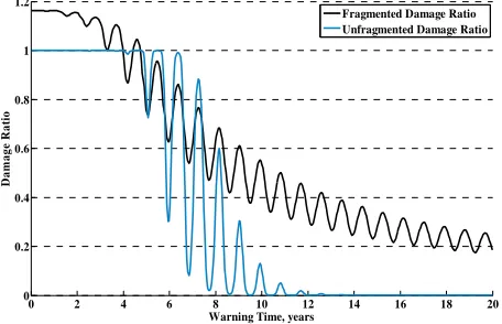
Fig. 16 shows the total damage ratio of the
fragmented Apophis, together with the ratio of the
unshattered object. The damage ratio of the fragmented case is computed by adding up the predicted weighted damage of each size, thus multiplying Table 3 damaged areas by results in Fig. 15, and then dividing the total area by the weighted damaged area of the
unfragmented Apophis, ∼40,000km2. We shall remind
that in this example the fragmentation was triggered by
a kinetic impactor with a ms/c of 10,000kg providing
500 j/kg of SKE. If Apophis would not shatter under
such a collisional energy the asteroid would be
deflected with a velocity of ∼
[
0.02m s/ 0 0]
,considering an enhancement factor β of 1. With this
change in velocity, Apophis would miss the Earth when
the minimum required change in velocity is smaller than 0.02 m/s, which occurs between 7 and 10 years (see Fig. 2). Fig. 16 shows the damage ratio of the unshattered object, which has been computed by
considering the change of velocity ∼
[
0.02m s/ 0 0]
with an added 25% error in both direction and modulus of to account for uncertainties during the mitigation mission, without this hypothetical error in the kinetic impactor performance, the damaged ratio would simply resembles a step function.
0 2 4 6 8 10 12 14 16 18 20 0
0.2 0.4 0.6 0.8 1 1.2
Warning Time, years
D
a
m
a
g
e
R
a
ti
o
[image:11.595.50.286.343.476.2]Fragmented Damage Ratio Unfragmented Damage Ratio
Fig. 16: Damage ratios of Apophis: fragmented case
(black line) and unfragmented case (blue line) with 25% error in the delta-velocity.
Fig. 16 demonstrates that if the outcome of a deflection mission is a barely catastrophic disruption
(fr=0.5), then there is a high probability to increase the
damage to the Earth, even for very long warning times.
6.4. Very catastrophic fragmentations events
Until now, we have assumed that a mitigation mission delivering 500j/kg was causing a disruption with fr=0.5. Clearly, if 500 j/kg is above the specific
energy for barely catastrophic disruption Q*, we should
[image:11.595.313.541.415.562.2]12
spawn a smaller number of dangerous fragments, thus reducing the damage ratio. Another interesting possible scenario would be using much higher levels of collisional energy with the solely purpose to fragment the threatening object providing higher levels of dispersion. In order to analyse these new scenarios, two
additional disruption fractions were used fr=0.25 and
fr=0.1, together with two more collisional energies,
1000 j/kg and 5000 j/kg.
0 2 4 6 8 10 12 14 16 18 20
0 0.2 0.4 0.6 0.8 1 1.2
Warning Time, years
D
a
m
a
g
e
R
a
ti
o
[image:12.595.54.284.173.329.2]fr=0.25 & 500j/kg fr=0.10 & 500j/kg fr=0.5 & 1000j/kg fr=0.25 & 1000j/kg fr=0.10 & 1000j/kg fr=0.5 & 5000j/kg fr=0.25 & 5000j/kg fr=0.10 & 5000j/kg Unfragmented Damage Ratio
Fig. 17: Damage ratios for a collisional energy of 500 j/kg with disruption levels at fr=0.25 and fr=0.1, and collisional energies of 1000 j/kg and 5000 j/kg with disruption levels at fr=0.5, fr=0.25 and fr=0.1.
Fig. 17 show 8 different scenarios with higher disruption levels and higher collisional energies. A
kinetic impactor with ms/c of 20,000kg could provide
1000j/kg of SKE to Apophis with an impact velocity
around 50km/s. Whereas to achieve 5000j/kg of SKE keeping the relative impact velocity of the impactor around 50km/s, i.e., velocities that are achievable with retrograde orbits, the mass of the kinetic impactor should be higher than 70,000kg. Although such an impact mass is highly improbable, a nuclear interceptor could provide the same level of energy with only a 1,000kg of spacecraft dry mass (mass of the spacrecraft without considering propellant), providing the similar change in velocity that a kinetic impactor with 70,000kg.
7. CONCLUSIONS
This work examined the risk of fragmentation that impulsive asteroid deflection mission, such as the kinetic impactor or the nuclear interceptor, can cause when attempting to deflect an asteroid in a single impulsive manoeuvre. A fragmentation and dispersion model was used to analyse the evolution of fragments for up to 20 years after the break-up of the asteroid. Using the probability that five different fragment sizes could impact with the Earth and the number of expected fragments resulting from a catastrophic
break-up of Apophis, the consequences of a
fragmentation were also studied for several illustrative examples.
The energies required for a single impulsive deflection manoeuvre, i.e, those of a kinetic impactor or nuclear interceptor, are dangerously close to the
energies required to catastrophically disrupt an asteroid. Even for relatively large warning times, more than 10 years prior to the collision, the risk of fragmentation seems considerable.
If an undesired fragmentation of the threatening object occurs, the risk to Earth is very high. For example, if a fragmentation is triggered while
attempting to deflect an asteroid similar to Apophis, 10
years prior to the collision, about half the total potential damage of the unfragmented asteroid could be still caused by the few fragments falling onto the Earth. Even if we attempt to fragment the asteroid with five times more energy than the minimum required to fragment an asteroid the damage to Earth is still significant.
8. REFERENCES
[1] Alvarez L.W., Alvarez W., Asaro F. and Michel H.V., "Extraterrestrial Cause for the
Cretaceous-Tertiary Extinction," Science, Vol. 208, No. 4448,
1980, pp. 1095-1108.
[2] Holsapple K.A., “The Scaling of Impact Processes
in Planetary Science,” Annual Review of Earth and
Planetary Science, Vol. 21, 1993, pp. 333-373.
[3] Ryan E.V. and Melosh H.J., "Impact
Fragmentation: From the Laboratory to Asteroids,"
Icarus, Vol. 133, No. 1, 1998, pp. 1-24.
[4] Melosh H.J., Nemchinov I.V. and Zetzer Y.I., "Non-nuclear Strategies for Deflecting Comets and
Asteroids," Hazard Due to Comets and Asteroids,
edited by T.Gehrels University of Arizona, 1994, pp. 1110-1131.
[5] Ivashkin V.V. and Smirnov V.V., "An Analysis of Some Methods of Asteroid Hazard Mitigation for
the Earth," Planetary and Space Science, Vol. 43,
No. 6, 1994, pp. 821-825.
[6] Remo J.L., "Energy Requirements and Payload
Masses for Near-Earth Objects Hazard
Mitigation," Acta Astronautica, Vol. 47, No. 1,
2000, pp. 35-50.
[7] "Near-Earth Objects Survey and Deflection Analysis of Alternatives," National Aeronautics and Space Administration, NASA Authorization Act of 2005, 2007.
[8] Sanchez J.P., Colombo C., Vasile M. and Radice G., "Multi-criteria Comparison among Several Mitigation Strategies for Dangerous Near Earth
Objects," Journal of Guidance, Control and
Dynamics, to appear, 2008.
[9] Ahrens T.J. and Harris A.W., "Deflection and
Fragmentation of Near-Earth Asteroids," Nature,
Vol. 360, 1992, pp. 429-433.
[10] Stokes G.H., Yeomans D.K., and et.al., "Study to
Determine the Feasibility of Extending the Search for Near-Earth Objects to Smaller Limiting Diameters," NASA, 2003.
[11] O'Brien D.P. and Greenberg R., "Steady-state size distributions for collisional populations: analytical
solution with size-dependent strength," Icarus,
Vol. 164, 2003, pp. 334-345.
13
results," Planetary and Space Science, Vol. 42, No. 12, 1994, pp. 1067-1078.
[13] Harris A.W., "The Rotation Rates of Very Small Asteroids: Evidence for 'Rubble Pile' Structure,"
Lunar and Planetary Science, Vol. 27, 1996, pp. 493.
[14] Chesley S.R. and Spahr T.B., "Earth Impactors: Orbital Characteristics and Warning Times,"
Mitigation of Hazardous Comets and Asteroids
2003.
[15] Vasile M. and Colombo C.. “Optimal Impact
Strategies for Asteroid Deflection,” Journal of
Guidance, Control and Dynamics, Vol.31, No.4, 2008.
[16]Tedeschi W.J., Remo J.L., Schulze J.F., and Young R.P., "Experimental Hypervelocity Impact Effects on Simulated Planetesimal Materials,"
International Journal of Impact Engineering, Vol. 17, 1995, pp. 837-848.
[17] McInnes C., "Deflection of Near-Earth Asteroids by kinetics Energy Impacts from Retrograde
Orbits," Planetary and Space Science, Vol. 52, No.
7, 2004, pp. 587-590.
[18] Petropoulos A.E., Kowalkowski T.D., Vavrina M.A., Parcher D.W., Finlayson P.A., Whiffen G. J. and Sims J.A., "1stACT global trajectory optimisation competition: Results found at the Jet
Propulsion Laboratory," Acta Astronautica, Vol.
61, 2007, pp. 806-815.
[19] Davis D.R. and Ryan E.V., "On Collisional Disruption: Experimental Results and Scaling
Laws," Icarus, Vol. 83, No. 156, 1990, pp. 182.
[20] H.Goldstein, Mecánica Clásica, 1996, pp.
518-520.
[21] Gault D.E., Shoemaker E. M., and Moore H.J., "Spray Ejected from the Lunar Surface by Meteoroid Impact," NASA Technical Note D-1767, 1963.
[22] Wiesel W., "Fragmentation of Asteroids and Artificial Satellites in Orbit," Icarus, 1978, pp. 99-116.
[23] Greenberg R., Wacker J.F., Hartmann W.K., and
Chapman C.R., "Planetesimal to Planets:
Numerical Simulations of Collisional Evolution,"
Icarus, Vol. 35, 1978, pp. 1-26.
[24] Mizutani H., Takagi Y. and Kawakami S.I., "New
Scaling Laws on Impact Fragmentation," Icarus,
Vol. 87, 1990, pp. 307-326.
[25] Hills J.G. and Goda M.P., "The Fragmentation of
Small Asteroids in the Atmosphere," The
Astronomical Journal, Vol. 105, No. 3, 1993, pp. 1114-1144.
[26]Chesley S.R. and Ward S.N., "A Quantitative Assessment of the Human and Economic Hazard
from Impact-generated Tsunami," Natural
Hazards, Vol. 38, 2006, pp. 355-374.
[27] Chapman C.R. and Morrison D., "Impacts on the Earth by asteroids and comets: assessing the
![Fig. 1: Critical Specific Energy Q* to barely catastrophically disrupt an asteroids with a diameter ranging from 40m to 1km using Ryan and Melosh [3] and Holsapple [12]](https://thumb-us.123doks.com/thumbv2/123dok_us/1712415.124629/2.595.316.544.297.469/critical-specific-energy-catastrophically-disrupt-asteroids-diameter-holsapple.webp)