Complexity of polarized spatial patterns in large area square VCSEL

arXiv:nlin.PS/0702004v1 1 Feb 2007

I.V. Babushkin

Max Born Institute for Nonlinear Optics and Short Pulse Spectroscopy, Max-Born-Str., 2a, D-12489, Berlin, Germany; Fax: +49 30 63921289; e-mail: [email protected]

N.A. Loiko

Institute of Physics, Academy of Sciences of Belarus, Scaryna Prospekt 70, 220072 Minsk, BELARUS; Fax: +375-172-393131; e-mail:[email protected]

T. Ackemann

SUPA and Department of Physics University of Strathclyde,

John Anderson Building, JA 8.21 107, Rottenrow, Glasgow G4 ONG, Scotland, UK; Fax: +44-(0)141-552 2891; e-mail: [email protected]

(Dated: February 2, 2007)

We consider pattern selection process in a wide aperture VCSEL near threshold. We show that for a square geometry of the laser aperture, the patterns formed at lasing threshold can be very complicated because of a possible misalignment between directions of an intrinsic spatial anisotropy of VCSEL and lateral boundaries of its aperture. The analogy with quantum billiard structures is established, and fingerprints of wave chaos are found. Influence of localized inhomogeneous in the pump current is also considered.

PACS numbers: 42.60.Jf, 42.65.Sf

I. INTRODUCTION

In the last decades, semiconductor laser devices have played an increasing role in scientific research and appli-cations. Among them, vertical cavity surface emitting lasers (VCSELs) can be distinguished, since these lasers emit normal to the wafer surface in the direction of epi-taxial growth. One of the features of VCSELs design is a possibility to mount extremely large (up to hundreds µm in diameter) aperture with high level of spatial ho-mogeneity. Spatial mode structures in such wide- aper-ture VCSELs have been a subject of many researches [1, 2, 3, 4, 5, 6, 7, 8, 9, 10, 11].

In general, the mechanism of pattern formation in VC-SEL is very complicated and involves both a complex structure of a VCSEL cavity (including Bragg reflectors) [10, 11, 12], as well as peculiarities of light-matter in-teraction in active quantum well semiconductor layers [15, 16, 17, 18, 19, 20]. However, near threshold one can invoke the perturbation theory and obtain normal forms governing the evolution of the system. It was shown recently, that due to a slight spatial anisotropy of a VCSEL cavity only a few spatial modes come into play at threshold and the shape of these modes can be analyzed by the linear approximation of the normal form [10, 11, 12] (in contrast to spatially isotropic systems, where the whole degenerate family of modes have the same critical growth rate at threshold, and the selection process requires consideration of nonlinear competition even at threshold [21, 22]). The investigations of the problem using this point of view was started in [12] for VCSELs with circular aperture. In that work, transition from the ’flower-like’ modes dictated by circular bound-aries to ’stripe-like’ ones, which are required by spatial

anisotropy of a VCSEL, was described.

In [12], the description was restricted to the light lin-ear polarized in direction coinciding with one of axes of the intrinsic laser anisotropy. In the present article, we extend this approach to the more general ”vectorial” case when the laser anisotropy is not so strong and both orthogonally polarized components of the field must be taken into account. This extension allows us to investi-gate the interaction of two polarization degrees of free-dom, that is important for the consideration of competi-tion of different mechanisms affecting pattern formacompeti-tion. The current research is motivated by the recent ex-perimental investigations [12, 13, 14], where it is shown that many aspects of spatial structures in VCSEL such as their transverse shape or frequency-versus-lengthscale dependence can be well described in a linear approxi-mation, which validates the ’linearized normal form’ ap-proach, used in this article.

We show here that this makes the structures at the laser threshold very complicated even in the case of a simple square aperture and perfectly manufactured VC-SEL cavity. The similar complexity was observed in the resent experimental investigations [4, 23, 24], where the scarred structures in the square broad-area VCSEL were obtained and treated as coherent states of quantum bil-liard. So, it is possible to speak in this context about ’quantum chaos’ in a wide aperture VCSEL.

cav-ity geometry [30]. Though the laser emission far from threshold is strongly affected by nonlinearities, the opti-cal spectra obey the same relations as a quantum billiard, governed by a linear Schr¨odinger equation.

We develop this approach further by considering the wide-aperture VCSEL near threshold as a kind of quan-tum billiard where the role of Hamilton operator is played by the operator of linearized order parameter equation for VCSEL. We show, that this operator is considerably more complicated than the transverse Laplace operator which is often used for consideration of quantum billiard systems. This leads to appearance of quantum chaos-like features, such as scarred orbits and nongaussian statistics of the levels even in the simple square geometry without a deformation of boundary conditions, that usually used for demonstrating quantum chaos features.

The structure of the article is following: in the sec-tion II we extend the approach used in [12] to take into account both orthogonally polarized components of the light field. In the section III we consider the pattern for-mation in VCSEL with a square geometry and discuss the influence of the polarization axes rotation against lateral boundaries of the cavity, as well as of slight spatial per-turbations of the pumping current. In the section IV we interpret our results in the ’quantum chaos’ framework.

II. THE VECTORIAL EIGENVALUE

PROBLEM

As has been pointed in the Introduction, the eigen-modes and their decay (or growth) rates can be directly obtained from a linear stability analysis of the nonlas-ing zero solution of the nonlinear equations governnonlas-ing VCSEL’s dynamics [10, 11, 12]. In comparison with a method when the field is decomposed into transverse eigenfunctions of the empty cavity [9, 31, 32], this ap-proach takes into account properties of a gain medium and of Bragg mirrors composing the cavity by the strick way.

For the infinitely large transverse-area devices the re-sulting eigenmodes are plane tilted waves (transverse Fourier modes) with the decay rates depending on the de-tuning of the longitudinal cavity resonance from the gain maximum and on a polarization of modes [10, 11, 33]. In contrast, the corresponding modes for the finite devices may be very complicated even in the scalar case. For example, for the circular aperture the modes can range from Bessel-like modes to the modes resembling more tilted waves [12].

The basic nonlinear equations for the vectorial case were obtained in [11] . The short description of these equations is given in Appendix A. The linearization pro-cedure is a generalization of one introduced in [12] to vectorial case, and is described in Appendix B. As in the scalar case, we linearize a complex nonlocal nonlinear operator, obtaining the linear but nonlocal pseudodiffer-ential operator (or speaking more precisely, certain

eigen-value problem for such operator) governing the field at threshold. Then, we approximate the operator describing the action of Bragg reflectors in transverse Fourier space and obtain the operator containing only partial deriva-tives up to fourth order. The total operator obtained af-ter such procedure includes main peculiarities of pataf-tern formation such as the dependence on detuning between longitudinal resonance of the cavity and gain peak fre-quency, and on the anisotropy of Bragg reflectors. This operator has the following form in the (x, y) space:

ˆ O=

4 X

i,j=0

aij ∂i+j

∂xi_yj +g00δµ(x, y) +ilδn(x, y). (1)

In contrast to the scalar case, for the vectorial case operator ˆO is a matrix, acting on the vectorial field

E _{= (Ex, Ey). Therefore, the coefficients aij are also}

2×2 matrices. We also consider inhomogeneities in the pumping currentδµ and in the indexδn, which play the role of disturbances. In the following, we mainly restrict ourself to only current inhomogeneities, because they are easier to be controlled.

EigenfunctionsE_{g and eigenvaluesλg of this operator}

are obtained by solving an eigenvalue problem:

ˆ

OE_{g(x, y)−λg}E_{g(x, y) = 0. (2)}

The eigenfunction corresponding to the eigenvalue with the largest real part determines a spatial field distribu-tion with maximal growth rate at threshold appearing after onset of generation. Aperture of the device has been simulated by zero field conditions on the bound-aries. Besides, because the operator ˆOis of fourth order, one should introduce an additional boundary condition which contains spatial derivatives of the field (see Ap-pendix B) to obtain the well posed eigenvalue problem. This second boundary condition can be chosen by differ-ent ways, but all them leads to approximately the same result [12]. Therefore, we select the second boundary condition appropriately, to simplify the solution (see Ap-pendix C).

The eigenvalue problem (2) is a generalization of more conventional one with transverse Laplace operator (6). The important difference however, is that the operator (1) is anisotropic, with a principal directions defined by polarization anisotropy of VCSEL cavity. It should be noted thatx-component of the fieldExandy-component of the fieldEy enters to Eq. (2) as just two components of a single vectorial eigenfunctionE_{g. In the following,}

III. COMPLEX SPATIAL STRUCTURES IN SQUARE-SHAPED VCSEL

A. Influence of alignment of boundaries and ansotropy direction

To elucidate the mechanism governing the pattern se-lection, we first consider the case of homogeneous pump-ing and index profile (δµ = 0, δn = 0). The presence of the aperture is modeled by zero boundary conditions. In this subsection we show, that the resulting spatio-temporal distribution strongly depends on the alignment of the boundary conditions and the main anisitropy axes of the device.

When boundaries and anisotropy directions are com-pletely aligned, the x-component of the first mode at threshold is a standing wave with stripes parallel to the direction of its polarization (see Fig. 1(a), (b)). Though the y-component is not zero due to the polarization mix-ing effect by Bragg reflectors, the couplmix-ing betweenxand ypolarizations is very week since for this case the Fourier transform of homogeneous part of ˆO,

O(k)= 4 X

i,j=0

(−i)i+jaijkixkyj. (3)

which is (kx, ky)-dependent 2x2 matrix, have nearly zero diagonal elements on the lineky = 0 andkx= 0. Thus, y-component is weaker in 100 times approximately for taken parameters.

If the boundaries are rotated with respect to the po-larization anisotropy direction, the stripes remain for a small rotation angleα, and their direction coincides with the boundaries rather then with anisotropy direction, i.e. they are rotated with the boundaries (see Fig. 1(e)-(h)). Structures of both polarized components are similar and their intensity become comparable.

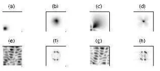
However, as α reaches some critical value, the corre-sponding structure becomes more complicated. Thus, for the parameter of Fig. 1(i)-(l), the spatial distribution of thex-polarized component of the field resembles stripes in the middle of the aperture, whereas near boundaries the pattern is more ’square-like’ one. At the same time, the structure of y-polarized component is more compli-cated and less regular. The critical angle for which stripes are giving place to complicated structures decreases with the size of the device, as well as with a value of anisotropy γa. However, stripes take place for relatively large size (composing of several tens of oscillation of the intensity). It should be noted that the structures presented in Fig. 1(i)-(l) are the combination of many transverse Fourier harmonics of different directions (see Fig. 1(j),(l)) in contrast to two travelling waves composing stripes for small α (Fig. 1(b),(f)).We show in the next section by considering the corresponding eigenvalue statistics, that such structures demonstrate some features which make them close to quantum chaos wavefunctions .

FIG. 1: The structures at threshold obtained as the eigen-vectors of ˆO(x,y) with the largest growth rate and different

angles of rotation of boundary against anisotropy directionα

(value ofabs(e) =√

I is plotted). (a)-(d) — anisotropy and boundaries are aligned (α= 0); (e)-(h) — the misalignment present (α=π/5); (i)-(l) — the misalignment has its largest possible value (α=π/4). (a),(e),(i) —x- component of the field polarization, (b),(f),(j) — its transverse Fourier trans-form; (c),(g),(k) — y- component of the field polarization, (d),(h),(l) — its transverse Fourier transform. The other rel-evant parameters are:l= 40µm γa= 0.01,γp= 0,δ= 30nm.

B. Influence of inhomogeneities

In this subsection, we consider an influence of pump inhomogeneities of different shape, amplitude and local-ization. As it was found earlier for devices with circular aperture [34], any slight inhomogeneities can change the sequence of a few first eigenfunctions in accordance with the order of their decay rates, preserving the shape of modes and their frequencies. In this connection, it is useful to investigate the subsequent eigenmodes of the linear eigenvalue problem (2).

FIG. 2: The second mode of homogeneous cavity with pa-rameters as in Fig.1 (e)-(h). It can be made first by adding small inhomogeneity in current δµ, which is localized near right boundary of the device.

is the splitting of the Fourier harmonics leading to the strong modulation of stripes in the near field (Fig.2 (b), (d)). The second eigenmode can be made leading one (one with the highest growth rate) by adding small inho-mogeneity to the currentδµ= 0.05δ(x, y), where δ(x, y) is a probe function which is nonzero in the vicinity of the right border and zero everywhere else.

If we decrease the detuningδbetween the gain maxima and the cavity resonance, the gain-loss dispersion mech-anism of Fourier harmonics selection becomes weaker [10, 11] and, as result, eigenmodes are more strongly de-termined by boundary conditions. The first mode for the large angle nearπ/4 does not have clear stripelike struc-tures in the center of device (Fig. 3 (a),(b)), and the sec-ond mode has the structure even less similar to stripes than previous one (Fig. 3 (c),(d)). However, stripelike structures do not disappear at all, as one can see in Fig. 3 (e),(f) for the next eigenmode. Moreover, the patterns with orthogonal direction of stripes can be easily exited (Fig. 3 (g),(h)). This could be explained by the fact that these two families of stripes are degenerate whenα= 0, and start to deviate from each other with increasingα.

FIG. 3: The first (a),(b); second (c,d); 5th and 6th eigen-modes of the device with the same parameters as in Fig. 1 but with smaller detuning (δ = 10nm), and angle of rota-tion of boundaries against anisotropy direcrota-tion is α = π/4. (a),(c),(e),(g) - x component of the field, (b),(d),(f),(h) - y

component of the field.

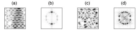
Some subsequent eigenmodes with larger decay rate for the same parameters are presented in Fig. 4. It is evident that for small enough (but nonzero) anisotropy the modes can differ from each other in their symmetry properties essentially, as in the case of circular aperture [12]. One can find nearly unordered structures (Fig. 4 (e)-(h)) and the structures which can be considered as ’scared’ eigenmodes of quantum billiard (Fig. 4 (a)-(d), (i)-(l)).

It is difficult to change the order of subsequent modes (especially to push one of them to the first position with highest grough rate) by introducing a small inhomogene-ity. Since stronger inhomogeneities needed for that mode structures can be changed also.

It should be also noted that whereas patterns of the orthogonally-polarized component (weaker component) of the laser field are usually of the same shape, one can find some exceptions (compare Fig. 4(i) and Fig. 4(k)).

FIG. 4: The subsequent eigenmodes for the same parameters as in Fig. 3. (a)-(d) - 7th (e)-(h) - 21th, (i)-(l) - 26th eigen-mode. (a),(e),(i) —x- component of the field polarization, (b),(f),(j) — its transverse Fourier transform; (c),(g),(k) —

y- component of the field polarization, (d),(h),(l) — its trans-verse Fourier transform.

However, even in this case the transverse Fourier images of the field components look quite similar. This is con-nected to the fact, that structures in both polarizations belong to the same eigenmode and coupled to each other in the absence of strong inhomogeneities through bound-ary conditions (they both and some combination of their derivatives must vanish at the boundary), and through the Bragg reflectors. The exception is only when this connection is very weak (Fig. 1 (a)-(d)).

FIG. 5: The first two eigenmodes for the device with the same parameters as in Fig. 1 (a)-(d), butδ= 8nm, and peak ofδµ

in the aperture. (a),(e) —x- component of the field polariza-tion, (b),(f) — its transverse Fourier transform; (c),(g) —y -component of the field polarization, (d),(h) — its transverse Fourier transform.

Up to now we have investigated the eigenmodes of ho-mogeneous devise, having in mind that the grough rate of a mode following the first one can become the largest one when a small perturbation of the currentδµis added, which does not sufficiently change the shape of mode.

changes in the shape of eigenmodes. As an example, we consider here strong inhomogeneities by introducing a peak or a hole into the laser aperture, that is quite natural for experiments.

For the peak in current profile, the first eigenmode is defined by this spot only, as if the rest of aperture is empty (Fig. 5 (a)-(d)). But, the subsequent modes fill all the cavity as there is no peak in the aperture at all (Fig. 5 (e)-(h)). However, they are more disordered then in the absence of inhomogeneity. The corresponding eigenvalues are also more separated as it is described in the next section.

FIG. 6: The first eigenmode for the same parameters as in Fig. 1 (a)-(d), but the boundary conditions (C5) are defined not on the boundaries of a square, but also on a circle inside the square (which creates the hole in the aperture). The hole is of 1/8 of the size of the laser and placed in the position (1/4,1/4) in the whole aperture. (a) —x- component of the field polarization, (b) — its transverse Fourier transform; (c) —y- component of the field polarization, (d) — its transverse Fourier transform.

On the other hand, if there is a strong hole in the current profile (which is for simplicity modeled by intro-ducing zero boundary conditions on the circle surround-ing the hole), the effect is not so visible, i.e. there is not a separation on the ”hole” mode and the rest ones. Moveover, the shape of eigenmodes for xpolarization is not changed so dramatically far from the hole (Fig. 6), although the structure of weak component is strongly dis-ordered comparing to the nonperturbed case (Fig. 1(c)). However, the subsequent eigenmodes are more irregular that the first one even for the x-component. The problem becomes close to chaotic one that could be considered in the framework of wave chaos.

IV. SIGNATURES OF QUANTUM CHAOS

Generally speaking, the term ’quantum chaos’ or ’wave chaos’ is usually attributed to investigation of quantum systems, which posses chaotic features in classical limit [25]. In contrast to classical systems, they obey linear evolution equation (Schr¨odinger equation). So, the ob-ject of investigation is usually the set of eigenvalues and eigenfunctions (stationary states) of some linear opera-tor, describing the quantum system under consideration (usually Hamilton operator). At that, the very important role is played by eigenvalue distribution, which shows fin-gerprints of chaos in quantum systems when the corre-sponding classical systems are chaotic.

Among the quantum systems, much attention is de-voted to the billiard systems [25, 35]. The quantum

coun-terpart of classical billiard is described by a wavefunction ψ(x, y, t), which obeys Schr¨odinger equation:

i~∂ψ

∂t = ∆ψ, (4)

with boundary condition

ψ= 0|_∂S, (5)

on the boundary of the domainS.

Stationary states of this problem are eigenfunctions of the transverse Laplace operator ∆ =_∂x∂22 +

∂2

∂y2:

i∆ψ=λψ. (6)

Depending on the shape of domain S, the correspond-ing classical problem can be either chaotic or regular. In the limit case of integrable system (for example, when the region has a rectangular shape), the corresponding eigen-value problem gives set of eigeneigen-values, obeying Poisson statistics of an eigenvalue spacings:

p(s) =exp(−s), (7)

where p(s) is a probability for corresponding value of eigenfrequency distributionsi= Im λi−Im λi+1.

For the opposite limit case of completely chaotic sys-tem, the corresponding distribution is the Wigner one:

p(s) = 1

2πsexp(− 1 4πs

2_{). (8)}

For intermediate situations one can define other statis-tic families limited by Eq. (7) and Eq. (8) [25, 36, 37]. One of fingerprints of quantum chaos in these intermedi-ate cases, as well as in the Eq. (8), that the maximum ofp(s) is reached fors6= 0. This defines so called level repulsion phenomena for chaotic systems.

The eigenfunctions of Hamilton operator also demon-strate fingerprints of chaos. In particular, one can ob-serve so called ’scarred’ patterns [23, 24, 38, 39, 40], which are localized near (unstable) periodic trajecto-ries of corresponding classical systems. Among the scared patterns, there are other eigenfunctions, which are strongly irregular and fit all the area.

It should be noted, that besides the quantum systems, the above mentioned framework is of the considerable interest for macro-systems, which are described at some level of approximation by Eq. (6) or Eq. (4). Among them are microwave billiards [25, 26, 27], microdisk lasers [28, 29] and VCSELs [23, 24, 30].

The eigenvalue statistics and other fingerprints of quantum chaos can give a criterion of a complexity of patterns near threshold. Indeed, if a system possess the Poisson statistics, the corresponding eigenfunctions are regular and stable against small perturbations, whereas for the Wigner one the eigenfunctions are much more irregular.

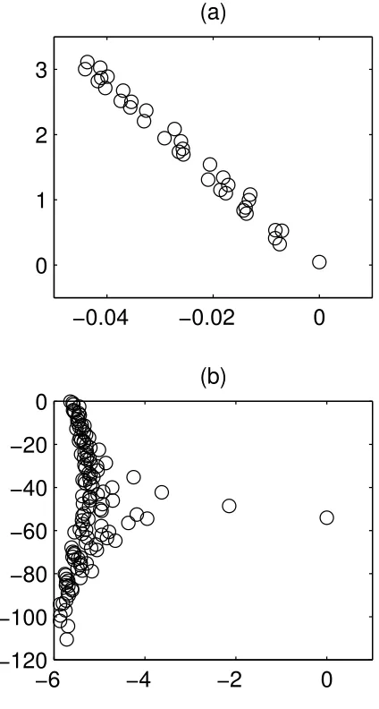
This operator is considerably more complicated then the transverse Laplace operator from Eq. (6). First of all, the eigenvalues of the operator ˆO are complex. Their real parts describe the decay rate of the corresponding eigenfunctions, whereas the complex parts are their os-cillation frequencies determining an energy level distribu-tion. Examples of the eigenvalues distribution are pre-sented in Fig. 7. For homogeneous device, all eigenvalues are concentrated along one line and in average their de-cay rates are increased with the frequencies (Fig. 7 (a)). The closeness of decay rates of the adjacent modes allows to change their order by a small perturbation. It is worth noting that for the taken parameters the eigenvalues are grouped in clusters and become deviate with decreasing of the angle α. In the case of a local peak in the pump current the eigenvalues distribution confirms the separa-tion of the first and the rest modes (Fig. 7 (b)).

−0.04

−0.02

0

0

1

2

3

(a)

−6

−4

−2

0

−120

−100

−80

−60

−40

−20

0

(b)

FIG. 7: (a) — Imaginary versus real part of few tens eigen-valuesλiof operator ˆOhaving the largest value of Re λi for VCSEL with parameters as in Fig. 1 (e)-(h). (b) — Imagi-nary versus real part of about hundred eigenvalues λi of ˆO for parameters close to ones used for Fig. 5.

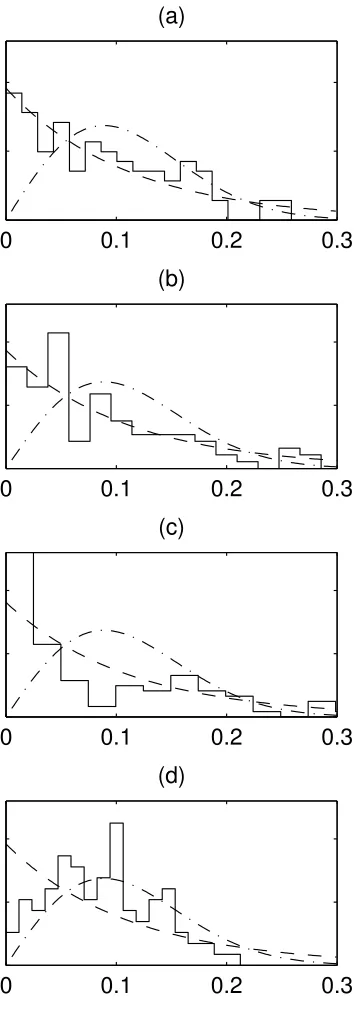
On the other hand, the operator (1) is anisotropic, with a preferential directions defined by anisotropy of VCSEL cavity. As one can see from (1),(2), if the boundaries are defined parallel toxand y axes, one can separate vari-ables in the eigenvalue problem and therefore it becomes integrable. Hence, as one can see in Fig. 8(a), when the boundaries and anisotropy direction coincides, the eigen-values obey more or less Poisson statistics.

When these two directions (anisotropy and boundaries for square shape of the aperture) are not aligned, the variable separation is not possible anymore (as would be for the second order differential operator). As a re-sult, forα 6= 0 (Fig. 8(b)) one can clearly see that the maximum probability of the level spacing distribution is shifted to nonzeros, possessing a fingerprint of wave chaos. However, the system can not be considered as purely ’quantum chaotic’ because the statistic is of inter-mediate type, neither purely Poisson nor Wigner one. It should be noted, that for isotropic system obeying Eq. (6) the eigenvalue spacing statistics remain Poisson for any values ofα. In our case, the eigenvalue spacing has the maximum value again at zero for the angleα=π/4, that can be explained by possible degeneracy of the operator

ˆ

O(Fig. 8(c)).

As a comparison the eigenlevel statistics is shown for boundary conditions of Fig. 6. It is clearly seen that for this case the statistics for spacing of imaginary parts of eigenvalues can be considered as Wigner one, which is quite expectable, because the same happens with the eigenvalues of the transverse Laplace operator. On the other hand, for the large peak in the aperture the eigenvalues do not obey the Wigner statistics anymore. For this case, the leading eigenvalues (eigenfunctions for which are shown in Fig. 5(a)-(d) and can be described as eigenvalues of a disturbance only) are strongly separated from others (which are resembling Fig. 5(e)-(h)), which obviously breaks the Wigner distribution.

The other signatures of complexity of spatial structures can be found in fingerprints of quantum chaos demon-strated by the shape of eigenfunctions. As one can see, the neighboring eigenmodes for misaligned boundaries and anisotropy directions (α6= 0) can differ sufficiently (Fig. 3, Fig. 4), including very irregular ones (Fig. 4(e)-(g)), which is a common property of systems possessing quantum chaos. On the other hand, beside complicated unordered structures, quantum chaos is characterized by ’scared’ eigenfunctions, which are located near unstable periodic trajectories of corresponding classical system. The example of eigenfunctions of operator ˆO, resembling that kind of structures (Fig. 4)(a)-(d),(i)-(l). Experimen-tally these structures were observed recently in VCSEL [23, 24].

V. DISCUSSION AND CONCLUSION

0

0.1

0.2

0.3

(a)

0

0.1

0.2

0.3

(b)

0

0.1

0.2

0.3

(c)

0

0.1

0.2

0.3

(d)

FIG. 8: The statistics of approximately 100 first eigenmodes (with largest value of Re λ) of VCSEL with parameters and boundaries as in Fig. 1 and Fig. 6, shown as stairstep graph, bold line. For a comparison Poisson statistics (Eq. 7) Wigner statistics (Eq. 8) is shown by dashed and dot-dashed lines, correspondingly. (a) corresponds to (a)-(d) in Fig. 1, i.e. α= 0, (b) corresponds to (e)-(h) in Fig. 1, i.e. α = π/5, (c) corresponds to (i)-(l) in Fig. 1, i.e. α=π/4, (d) corresponds to complicated region of Fig. 6.

Bragg reflectors, the presence of polarization anisotropy creates a spatial anisotropy. This allows to investigate the structure of pattern near threshold by linearized or-der parameter equations, since even in a linear approxi-mation the mode with the smallest decay rate is nonde-generate (in contrast to spatially isotropic systems, where the whole family of modes has the same growth rate at threshold, and nonlinear competition is of strong impor-tance for the selection). Since our studies concentrated on a VCSEL with square aperture, the competition of boundary direction (which can be defined as a vector, parallel to one of the sides of the square), and spatial anisotropy is important mechanism for pattern selection.

To measure the complexness of a pattern structure we use criteria from the topic of quantum chaos, where the main object of research is also an eigenvalue problem of some operator. One of fingerprints of complicated be-havior is an eigenvalue spacing statistics.

In this work we have considered a statistics of imagi-nary parts of eigenvalues, describing frequencies of cor-responding eigenfunctions. We have shown that in the case of aligned directions of boundaries and spatial (or polarization) anisotropy, the above mentioned statistics is close to Poisson one. However, when the angle of rota-tion of spatial anisotropy against boundaries is not zero, the statistics is not Poisson anymore. In the later case, the statistics shows a signature of level spacing repulsion, i.e. maximum of eigenspacing distribution is not zero.

The other fingenprints of quantum chaos can be found in the spatial shape of eigenfunctions, which can be very irregular, as well as ’scared-like’ patterns.

To compare these results with experiments, we also have investigated the influence of the inhomogeneities. The considered system is stable in the sense, that small perturbations only change the modes order preserving their shape, and not lead to dramatic change of the whole picture. In this sense, the consideration of subsequent modes (having higher decay rate) are also important, be-cause they can be considered as leading ones of the device perturbed by some (may be unknown) inhomogeneity.

Acknowledgments

This work was financially supported by the Deutsche Forschungsgemeinschaft for equipment and by travel grants. We are grateful to Malte Schutz-Ruhtenberg for useful discussions.

APPENDIX A: BASIC SYSTEM

The system under consideration was initially obtained in [11]. The equations for the fieldE_{= (Ex, Ey) take into}

account propagation inside the complex VCSEL cavity. The material equations are based on spin-flip model [41], describing four level system with populations differences of relevant transitions determined by their sum N and differencen:

dE_{(xt, t)}

dt = −κMˆE+iΩˆE−ΓˆE−iκαE+κ(1 +iα) ˆGLˆΩ( ˆAE), (A1) dN

dt = −N+µ−Im[(i−α)E ∗_Lˆ

Ω( ˆAE)], (A2)

dn

dt = −γsd−Re[(i−α)E

∗_Lˆ_{Ω( ˆA}E_{)], (A3)}

(A4)

where

A =

N in −in N

,

and the operators ˆM and ˆG describes the modal losses and gain, correspondingly, ˆΩ describes the influence of the diffraction in the complex resonator of VCSEL. These operators take into account the influence of reflection from Bragg reflectors and are quite complicated. More details can be found in [11, 12].

The operator

ˆ LΩ= 1/



1 +

δ−Ωˆ γ

!2



describes the Lorentz shape of gain contour with a detun-ing δ between the gain maximum and cavity resonance frequency. κis the field decay rate in the VCSEL’s cavity. The operator ˆΓ describes the inner anisotropy of VC-SEL’s cavity:

ˆ Γ₌

exp(γa+iγp) 0

0 exp(−(γa+iγp))

where γa and γp is an amplitude and phase anisotropy, respectively.

APPENDIX B: VECTORIAL EIGENVALUE PROBLEM DERIVATION

To derive the linear evolution equation in the form, ∂E

∂t = ˆOEg(x, y), (B1)

(which is then reduced to Eq. 2) using the basic equations (A1-A3), we take into account that at the laser thresh-old two branches of the steady state solutions cross each other: the zero solution (E_{= 0), and the nonzero lasing}

one. Because of the lasing solution at the cross-section point is characterized byE _{= 0 and N =µthe further}

analysis is drastically simplified giving the following di-agonal operator of the linearized problem:

ˆ T =

_Oˆ 11 0

0 Oˆ₂₂

. (B2)

where each ˆOii is in turn the matrix operator:

ˆ Oii=

ˆ O(11ii) Oˆ

(ii) 12

ˆ

O(₂₁ii) Oˆ(₂₂ii)

!

. (B3)

The diagonal form of (B2) shows, that the fieldE_and

the variablesN,n are independent of each other at the laser threshold, and the spectrum for ˆO22lies entirely in

the half-plane Re λ≤0, hence we can consider only the equation for the field Eq. B1 with ˆO≡Oˆ11. ˆO includes

ˆ

O=−κMˆ +iΩˆ−Γˆ−iκα+κ(1 +iα)µGˆLˆΩ. (B4)

However, the expression (B4) is still nonlocal, because all the operators in (B4) are integrodifferential. The equation can be made local in the manner of [12]. The procedure used for a scalar operator in [12], must be ap-plied to each of the operatorsO_ij(11), which are the scalar components of ˆO. Because the diagonal part of (B3) plays the main role, it is approximated up to the fourth order of k_{⊥, whereas the operators O}(11)

ij for i 6= j are approximated with terms of the second order ofk_⊥.

In the presence of index inhomogeneities, ˆΩ = Ωhomogen+ilδn (where l =τ ω/n0 is expressed via the

optical frequencyω, round trip time of the cavityτand the mean index n0. The pump current inhomogeneities

have to be included in the coefficient of the last term µ=µhomogen+δµ.

APPENDIX C: NUMERICAL IMPLEMENTATION OF EIGENVALUE

PROBLEM

To solve the problem, the Matlab PDE toolbox imple-mentation [42] of Arnoldi method for the system of par-tial differenpar-tial equations of the second order has been used. For that, the operators of the fourth order ˆO(11)_ii have been represented via multiplication of two operators

ˆ

Pi1, ˆPi2 of the second order with constant coefficients:

ˆ

O(11)ii = ˆPi1Pˆi2−li1= ˆPi2Pˆi1−li1 (C1)

wherePi1=∇ ·(c(12i)⊗ ∇),Pi2=∇ ·(c(21i)⊗ ∇).

Herec(_ijk)are matrices defined by formulas given in [12] using the coefficientsaij (to definec(1)ij andc

(2)

ij the coef-ficients (aij)(11) and (aij)(22)are used, correspondingly).

Then, defining a new vector variable

E_{1= ( ˆP12Ex,P}ˆ_{22Ey) (C2)}

or

E_{1= ( ˆP11Ex,P}ˆ_{21Ey) (C3)}

one can present the action of the operator of fourth order ˆ

O(x,y)as a operator of the second order of the type

ˆ

P =∇ ·(c⊗ ∇) +a. (C4)

acting on a four-component function E_{ex = (}E_,E_1).

Hereais a 4×4 matrix (instead of 2×2 for scalar case [12]), c is a rank four tensor which can be described by eight 2×2 matricesc(_ijk), mentioned above after equation (C1). The boundary conditions have to be also general-ized for the functionE_{ex as in the work [12]:}

E_{ex= 0 :}E_{= 0,}E_{1= 0, (C5)}

whereE_{1 is defined by (C2) or (C3).}

In the framework of the original system it means that we introduce a second boundary conditions on the vector fieldE _{in accordance with that the operator ˆO(x,y) is of}

the fourth order.

[1] S. Hegarty, G. Huyet, J. G. McInerney, and K. D. Cho-quette, Phys. Rev. Lett.82, 1434 (1999).

[2] J. Scheuer and M. Orenstein, Science285, 230 (1999). [3] T. Ackemannet al., J. Opt. B: Quantum Semiclass. Opt.

2, 406 (2000).

[4] K. F. Huang, Y. F. Chen, H. C. Lai, and Y. P. Lan, Phys. Rev. Lett.89, 224102 (2002).

[5] C. J. Chang-Hasnain et al., Appl. Phys. Lett. 57, 218 (1990).

[6] H. Li, T. L. Lucas, J. G. McInerney, and R. A. Morgan, Chaos, Solitons & Fractals4, 1619 (1994).

[7] I. H¨orschet al., J. Appl. Phys.79, 3831 (1996).

[8] M. Grabherret al., IEEE Photon. Technol. Lett.10, 1061 (1998).

[9] C. Degenet al., Phys. Rev. A63, 23817 (2001). [10] N. A. Loiko and I. V. Babushkin, Quantum Electronics

31, 221 (2001).

[11] N. A. Loiko and I. V. Babushkin, J. Opt. B: Quantum

Semiclass. Opt.3, S234 (2001).

[12] I. V. Babushkin, N. A. Loiko, and T. Ackemann, Phys. Rev. E69, 066205 (2004).

[13] M. Schulz-Ruhtenberg, I. V. Babushkin, N. A. Loiko, T. Ackemann, and K. F. Huang Appl. Phys. B81, 945 (2005).

[14] M. Schulz-Ruhtenberg, T. Ackemann Unpublished. [15] D. Burak, J. V. Moloney, and R. Binder, Phys. Rev. A

61, 053809 (2000).

[16] D. Burak, J. V. Moloney, and R. Binder, IEEE J. Quan-tum Electron.36, 956 (2000).

[17] C. Degen, I. Fischer, and W. Els¨aßer, Appl. Phys. Lett.

76, 3352 (2000).

[18] C. Degenet al., J. Opt. B: Quantum Semiclass. Opt.2, 517 (2000).

[19] C. Z. Ning and J. V. Moloney, Opt. Lett.20, 1151 (1995). [20] T. R¨ossler, R. A. Indik, G. K. Harkness, and J. V.

[21] J. Lega, J. Moloney, and A. Newell, Physica D 83, 478 (1995).

[22] F. T. Arecchi, S. Boccaletti, and P. L. Ramazza, Phys. Rep.318, 1 (1999).

[23] Y. F. Chen, K. F. Huang, and Y. P. Lan, Phys. Rev. E

66, 046215 (2002).

[24] Y. F. Chen, K. F. Huang, H. C. Lai, and Y. P. Lan, Phys. Rev. Lett.90, 053904 (2003).

[25] H.-J. St¨ockmann, Quantum Chaos — an Introduction (Cambrige University Press, Marburg, 1999).

[26] H.-J. St¨ockmann and J. Stein, Phys. Rev. Lett.64, 2215 (1990).

[27] H.-D. Gr¨afet al., Phys. Rev. Lett.69, 1296 (1992). [28] J. U. N¨ockel and D. Stone, Nature385, 45 (1997). [29] T. Harayama, P. Davis, and K. S. Ikeda, Phys. Rev. Lett.

90, 063901 (2003).

[30] T. Genstyet al., Phys. Rev. Lett.94, 233991 (2005). [31] L. A. Coldren and S. W. Corzine,Diode Lasers and

Pho-tonic Integrated Circuits(Wiley, New York, 1995).

[32] J. Mulet and S. Balle, IEEE J. Quantum Electron.38, 291 (2002).

[33] T. R¨ossler, J. V. Moloney, and T. Ackemann, (2003), submitted to Phys. Rev. A.

[34] I. V. Babushkin, N. A. Loiko, and T. Ackemann, Phys. Rev. A67, 013813 (2003).

[35] P. Cvitanovi´cet al., Classical and Quantum Chaos, 2004. [36] F. Izrailev, Phys. Lett. A134, 13 (1988).

[37] T. Brody, Lett. Nuovo Cimento7, 482 (1973). [38] E. J. Heller, Phys. Rev. Lett.53, 1515 (1991). [39] E. B. Bogomolny, Physica D31, 169 (1988).

[40] M. V. Berry, Proc. R. Soc. Lond. A423, 219 (1989). [41] M. San Miguel, inSemiconductor quantum

optoelectron-ics: From quantum physics to smart devices, edited by A. Miller, M. Ebrahimzadeh, and D. M. Finlayson (SUSSP and Institute of Physics Publishing, Bristol, 1999), pp. 339–366.