Upper limits on gravitational wave emission from 78 radio pulsars

arXiv:gr-qc/0702039v1 7 Feb 2007

LIGO-P060011-03-Z

Upper limits on gravitational wave emission from 78 radio pulsars

B. Abbott,14 _{R. Abbott,}14 _{R. Adhikari,}14 _{J. Agresti,}14 _{P. Ajith,}2 _{B. Allen,}50 _{R. Amin,}18 _{S. B. Anderson,}14

W. G. Anderson,50 _{M. Arain,}39_{M. Araya,}14_{H. Armandula,}14 _{M. Ashley,}4 _{S Aston,}38 _{P. Aufmuth,}35 _{C. Aulbert,}1

S. Babak,1 _{S. Ballmer,}14 _{H. Bantilan,}8 _{B. C. Barish,}14 _{C. Barker,}16 _{D. Barker,}16 _{B. Barr,}40 _{P. Barriga,}49

M. Barton,40 _{K. Bayer,}15_{J. Betzwieser,}15 _{P. T. Beyersdorf,}27 _{B. Bhawal,}14, a _{I. A. Bilenko,}21 _{G. Billingsley,}14

R. Biswas,50_{E. Black,}14 _{K. Blackburn,}14 _{L. Blackburn,}15 _{D. Blair,}49 _{B. Bland,}16 _{J. Bogenstahl,}40 _{L. Bogue,}17

R. Bork,14 _{V. Boschi,}14 _{S. Bose,}51 _{P. R. Brady,}50_{V. B. Braginsky,}21 _{J. E. Brau,}43_{M. Brinkmann,}2_{A. Brooks,}37

D. A. Brown,14 _{A. Bullington,}30 _{A. Bunkowski,}2_{A. Buonanno,}41 _{O. Burmeister,}2 _{D. Busby,}14 _{R. L. Byer,}30

L. Cadonati,15 G. Cagnoli,40J. B. Camp,22 J. Cannizzo,22K. Cannon,50C. A. Cantley,40J. Cao,15 L. Cardenas,14 G. Castaldi,46_{C. Cepeda,}14 _{E. Chalkey,}40_{P. Charlton,}9_{S. Chatterji,}14 _{S. Chelkowski,}2 _{Y. Chen,}1 _{F. Chiadini,}45

N. Christensen,8 _{J. Clark,}40_{P. Cochrane,}2 _{T. Cokelaer,}7 _{R. Coldwell,}39_{R. Conte,}45_{D. Cook,}16 _{T. Corbitt,}15

D. Coyne,14J. D. E. Creighton,50 R. P. Croce,46D. R. M. Crooks,40A. M. Cruise,38A. Cumming,40 J. Dalrymple,31 E. D’Ambrosio,14 _{K. Danzmann,}35, 2 _{G. Davies,}7 _{D. DeBra,}30 _{J. Degallaix,}49 _{M. Degree,}30 _{T. Demma,}46

V. Dergachev,42_{S. Desai,}32_{R. DeSalvo,}14_{S. Dhurandar,}13_{M. D´ıaz,}33_{J. Dickson,}4_{A. Di Credico,}31_{G. Diederichs,}35

A. Dietz,7 _{E. E. Doomes,}29 _{R. W. P. Drever,}5_{J.-C. Dumas,}49 _{R. J. Dupuis,}14 _{J. G. Dwyer,}10 _{P. Ehrens,}14

E. Espinoza,14_{T. Etzel,}14 _{M. Evans,}14 _{T. Evans,}17 _{S. Fairhurst,}7, 14 _{Y. Fan,}49 _{D. Fazi,}14 _{M. M. Fejer,}30

V. Fiumara,45 _{L. S. Finn,}32 _{N. Fotopoulos,}50 _{A. Franzen,}35 _{K. Y. Franzen,}39, b _{A. Freise,}38 _{R. E. Frey,}43

T. Fricke,44_{P. Fritschel,}15 _{V. V. Frolov,}17_{M. Fyffe,}17 _{V. Galdi,}46 _{J. Garofoli,}16 _{I. Gholami,}1_{J. A. Giaime,}17, 18

S. Giampanis,44 _{K. D. Giardina,}17 _{K. Goda,}15 _{E. Goetz,}42 _{L. Goggin,}14_{G. Gonz´alez,}18_{S. Gossler,}4 _{A. Grant,}40

S. Gras,49_{C. Gray,}16 _{M. Gray,}4_{J. Greenhalgh,}26 _{A. M. Gretarsson,}11_{R. Grosso,}33, c _{H. Grote,}2 _{S. Grunewald,}1

M. Guenther,16 _{R. Gustafson,}42 _{B. Hage,}35 _{D. Hammer,}50 _{C. Hanna,}18 _{J. Hanson,}17_{J. Harms,}2_{G. Harry,}15

E. Harstad,43_{T. Hayler,}26_{J. Heefner,}14 _{I. S. Heng,}40 _{A. Heptonstall,}40_{M. Heurs,}2 _{M. Hewitson,}2 _{S. Hild,}35

E. Hirose,31_{D. Hoak,}17 _{D. Hosken,}37 _{J. Hough,}40_{D. Hoyland,}38_{S. H. Huttner,}40 _{D. Ingram,}16 _{E. Innerhofer,}15

M. Ito,43 _{Y. Itoh,}50 _{A. Ivanov,}14 _{B. Johnson,}16 _{W. W. Johnson,}18 _{D. I. Jones,}40, d _{G. Jones,}7 _{R. Jones,}40 _{L. Ju,}49

P. Kalmus,10 _{V. Kalogera,}24_{D. Kasprzyk,}38 _{E. Katsavounidis,}15_{K. Kawabe,}16 _{S. Kawamura,}23 _{F. Kawazoe,}23

W. Kells,14 _{D. G. Keppel,}14 _{F. Ya. Khalili,}21_{C. Kim,}24_{P. King,}14 _{J. S. Kissel,}18 _{S. Klimenko,}39_{K. Kokeyama,}23

V. Kondrashov,14 _{R. K. Kopparapu,}18_{D. Kozak,}14 _{B. Krishnan,}1_{P. Kwee,}35_{P. K. Lam,}4_{M. Landry,}16_{B. Lantz,}30

A. Lazzarini,14_{M. Lei,}14_{J. Leiner,}51 _{V. Leonhardt,}23_{I. Leonor,}43_{K. Libbrecht,}14 _{P. Lindquist,}14_{N. A. Lockerbie,}47

M. Longo,45_{M. Lormand,}17_{M. Lubinski,}16 _{H. L¨uck,}35, 2 _{B. Machenschalk,}1 _{M. MacInnis,}15 _{M. Mageswaran,}14

K. Mailand,14 _{M. Malec,}35, e _{V. Mandic,}14 _{S. Marano,}45 _{S. M´arka,}10 _{J. Markowitz,}15_{E. Maros,}14 _{I. Martin,}40

J. N. Marx,14 _{K. Mason,}15_{L. Matone,}10 _{V. Matta,}45 _{N. Mavalvala,}15_{R. McCarthy,}16 _{D. E. McClelland,}4

S. C. McGuire,29 _{M. McHugh,}20 _{K. McKenzie,}4 _{S. McWilliams,}22 _{T. Meier,}35 _{A. Melissinos,}44 _{G. Mendell,}16

R. A. Mercer,39 _{S. Meshkov,}14 _{E. Messaritaki,}14_{C. J. Messenger,}40 _{D. Meyers,}14 _{E. Mikhailov,}15 _{S. Mitra,}13

V. P. Mitrofanov,21 _{G. Mitselmakher,}39 _{R. Mittleman,}15 _{O. Miyakawa,}14_{S. Mohanty,}33 _{G. Moreno,}16_{K. Mossavi,}2

C. MowLowry,4 _{A. Moylan,}4 _{G. Mueller,}39 _{S. Mukherjee,}33_{H. M¨uller-Ebhardt,}2 _{J. Munch,}37 _{P. Murray,}40

E. Myers,16_{J. Myers,}16_{G. Newton,}40 _{A. Nishizawa,}23 _{K. Numata,}22 _{B. O’Reilly,}17 _{R. O’Shaughnessy,}24

D. J. Ottaway,15 _{H. Overmier,}17 _{B. J. Owen,}32 _{Y. Pan,}41 _{M. A. Papa,}1, 50 _{V. Parameshwaraiah,}16

P. Patel,14 _{M. Pedraza,}14 _{S. Penn,}12 _{V. Pierro,}46 _{I. M. Pinto,}46_{M. Pitkin,}40 _{H. Pletsch,}50 _{M. V. Plissi,}40

F. Postiglione,45_{R. Prix,}1 _{V. Quetschke,}39_{F. Raab,}16_{D. Rabeling,}4 _{H. Radkins,}16 _{R. Rahkola,}43_{N. Rainer,}2

M. Rakhmanov,32 _{S. Ray-Majumder,}50 _{V. Re,}38, f _{H. Rehbein,}2 _{S. Reid,}40 _{D. H. Reitze,}39 _{L. Ribichini,}2

R. Riesen,17 _{K. Riles,}42 _{B. Rivera,}16 _{N. A. Robertson,}14, 40 _{C. Robinson,}7 _{E. L. Robinson,}38 _{S. Roddy,}17

A. Rodriguez,18 _{A. M. Rogan,}51 _{J. Rollins,}10 _{J. D. Romano,}7_{J. Romie,}17 _{R. Route,}30_{S. Rowan,}40_{A. R¨udiger,}2

L. Ruet,15 _{P. Russell,}14 _{K. Ryan,}16 _{S. Sakata,}23 _{M. Samidi,}14 _{L. Sancho de la Jordana,}36_{V. Sandberg,}16

V. Sannibale,14 _{S. Saraf,}25_{P. Sarin,}15_{B. S. Sathyaprakash,}7 _{S. Sato,}23_{P. R. Saulson,}31 _{R. Savage,}16 _{P. Savov,}6

S. Schediwy,49 _{R. Schilling,}2 _{R. Schnabel,}2 _{R. Schofield,}43 _{B. F. Schutz,}1, 7 _{P. Schwinberg,}16 _{S. M. Scott,}4

A. C. Searle,4 _{B. Sears,}14 _{F. Seifert,}2_{D. Sellers,}17_{A. S. Sengupta,}7 _{P. Shawhan,}41_{D. H. Shoemaker,}15_{A. Sibley,}17

J. A. Sidles,48 _{X. Siemens,}14 _{D. Sigg,}16 _{S. Sinha,}30 _{A. M. Sintes,}36, 1 _{B. Slagmolen,}4 _{J. Slutsky,}18 _{J. R. Smith,}2

M. R. Smith,14 _{K. Somiya,}2, 1 _{K. A. Strain,}40 _{D. M. Strom,}43 _{A. Stuver,}32 _{T. Z. Summerscales,}3_{K.-X. Sun,}30

M. Sung,18 _{P. J. Sutton,}14 _{H. Takahashi,}1_{D. B. Tanner,}39 _{R. Taylor,}14 _{R. Taylor,}40 _{J. Thacker,}17_{K. A. Thorne,}32

K. S. Thorne,6 _{A. Th¨uring,}35 _{K. V. Tokmakov,}40_{C. Torres,}33_{C. Torrie,}40 _{G. Traylor,}17 _{M. Trias,}36 _{W. Tyler,}14

D. Ugolini,34 _{K. Urbanek,}30_{H. Vahlbruch,}35 _{M. Vallisneri,}6 _{C. Van Den Broeck,}7_{M. Varvella,}14, g _{S. Vass,}14

A. Vecchio,38 _{J. Veitch,}40 _{P. Veitch,}37 _{A. Villar,}14 _{C. Vorvick,}16_{S. P. Vyachanin,}21 _{S. J. Waldman,}14 _{L. Wallace,}14

J. T. Whelan,1 _{S. E. Whitcomb,}14 _{B. F. Whiting,}39 _{C. Wilkinson,}16 _{P. A. Willems,}14 _{L. Williams,}39

B. Willke,35, 2 _{I. Wilmut,}26 _{W. Winkler,}2 _{C. C. Wipf,}15 _{S. Wise,}39 _{A. G. Wiseman,}50_{G. Woan,}40 _{D. Woods,}50

R. Wooley,17 _{J. Worden,}16 _{W. Wu,}39 _{I. Yakushin,}17 _{H. Yamamoto,}14 _{Z. Yan,}49 _{S. Yoshida,}28 _{N. Yunes,}32

M. Zanolin,15_{J. Zhang,}42 _{L. Zhang,}14_{C. Zhao,}49 _{N. Zotov,}19 _{M. Zucker,}15 _{H. zur M¨uhlen,}35 _{and J. Zweizig}14

(The LIGO Scientific Collaboration, http://www.ligo.org)

M. Kramer52 _{and A. G. Lyne}52

1_{Albert-Einstein-Institut, Max-Planck-Institut f¨ur Gravitationsphysik, D-14476 Golm, Germany}

2_{Albert-Einstein-Institut, Max-Planck-Institut f¨ur Gravitationsphysik, D-30167 Hannover, Germany}

3_{Andrews University, Berrien Springs, MI 49104 USA}

4_{Australian National University, Canberra, 0200, Australia}

5_{California Institute of Technology, Pasadena, CA 91125, USA}

6_{Caltech-CaRT, Pasadena, CA 91125, USA}

7_{Cardiff University, Cardiff, CF2 3YB, United Kingdom}

8_{Carleton College, Northfield, MN 55057, USA}

9_{Charles Sturt University, Wagga Wagga, NSW 2678, Australia}

10_{Columbia University, New York, NY 10027, USA}

11_{Embry-Riddle Aeronautical University, Prescott, AZ 86301 USA}

12_{Hobart and William Smith Colleges, Geneva, NY 14456, USA}

13_{Inter-University Centre for Astronomy and Astrophysics, Pune - 411007, India}

14_{LIGO - California Institute of Technology, Pasadena, CA 91125, USA}

15_{LIGO - Massachusetts Institute of Technology, Cambridge, MA 02139, USA}

16_{LIGO Hanford Observatory, Richland, WA 99352, USA}

17_{LIGO Livingston Observatory, Livingston, LA 70754, USA}

18_{Louisiana State University, Baton Rouge, LA 70803, USA}

19_{Louisiana Tech University, Ruston, LA 71272, USA}

20_{Loyola University, New Orleans, LA 70118, USA}

21_{Moscow State University, Moscow, 119992, Russia}

22_{NASA/Goddard Space Flight Center, Greenbelt, MD 20771, USA}

23_{National Astronomical Observatory of Japan, Tokyo 181-8588, Japan}

24_{Northwestern University, Evanston, IL 60208, USA}

25_{Rochester Institute of Technology, Rochester, NY 14623, USA}

26_{Rutherford Appleton Laboratory, Chilton, Didcot, Oxon OX11 0QX United Kingdom}

27_{San Jose State University, San Jose, CA 95192, USA}

28_{Southeastern Louisiana University, Hammond, LA 70402, USA}

29_{Southern University and A&M College, Baton Rouge, LA 70813, USA}

30_{Stanford University, Stanford, CA 94305, USA}

31_{Syracuse University, Syracuse, NY 13244, USA}

32_{The Pennsylvania State University, University Park, PA 16802, USA}

33_{The University of Texas at Brownsville and Texas Southmost College, Brownsville, TX 78520, USA}

34_{Trinity University, San Antonio, TX 78212, USA}

35_{Universit¨at Hannover, D-30167 Hannover, Germany}

36_{Universitat de les Illes Balears, E-07122 Palma de Mallorca, Spain}

37_{University of Adelaide, Adelaide, SA 5005, Australia}

38_{University of Birmingham, Birmingham, B15 2TT, United Kingdom}

39_{University of Florida, Gainesville, FL 32611, USA}

40_{University of Glasgow, Glasgow, G12 8QQ, United Kingdom}

41_{University of Maryland, College Park, MD 20742 USA}

42_{University of Michigan, Ann Arbor, MI 48109, USA}

43_{University of Oregon, Eugene, OR 97403, USA}

44_{University of Rochester, Rochester, NY 14627, USA}

45_{University of Salerno, 84084 Fisciano (Salerno), Italy}

46_{University of Sannio at Benevento, I-82100 Benevento, Italy}

47_{University of Strathclyde, Glasgow, G1 1XQ, United Kingdom}

48_{University of Washington, Seattle, WA, 98195}

49_{University of Western Australia, Crawley, WA 6009, Australia}

50_{University of Wisconsin-Milwaukee, Milwaukee, WI 53201, USA}

51_{Washington State University, Pullman, WA 99164, USA}

52_{University of Manchester, Jodrell Bank Observatory, Macclesfield, Cheshire, SK11 9DL, United Kingdom}

We present upper limits on the gravitational wave emission from 78 radio pulsars based on data from the third and fourth science runs of the LIGO and GEO 600 gravitational wave detectors. The data from both runs have been combined coherently to maximise sensitivity. For the first time pulsars within binary (or multiple) systems have been included in the search by taking into account the signal modulation due to their orbits. Our upper limits are therefore the first measured for 56 of these pulsars. For the remaining 22, our results improve on previous upper limits by up to a factor of 10. For example, our tightest upper limit on the gravitational strain is 3.2×10−25 _for

PSR J1603−7202, and the equatorial ellipticity of PSR J2124−3358 is less than 10−6_{. Furthermore,}

our strain upper limit for the Crab pulsar is only three times greater than the fiducial spin-down limit.

PACS numbers: 04.80.Nn, 95.55.Ym, 97.60.Gb, 07.05.Kf

I. INTRODUCTION

This paper details the results of a search for gravita-tional wave signals from known radio pulsars in data from the third and fourth LIGO and GEO 600 science runs (de-noted S3 and S4). These runs were carried out from 31st

October 2003 to 9th _{January 2004 and 22}nd _{February to}

23rd _{March, 2005 respectively. We have applied, and}

ex-tended, the search technique of Dupuis and Woan [1] to generate upper limits on the gravitational wave ampli-tude from a selection of known radio pulsars, and infer upper limits on their equatorial ellipticities. The work is a natural extension our previous work given in Refs. [2, 3].

A. Motivation

To emit gravitational waves a pulsar must have some mass (or mass-current) asymmetry around its rotation axis. This can be achieved through several mechanisms such as elastic deformations of the solid crust or core or distortion of the entire star by an extremely strong misaligned magnetic field (see Sec. III of Ref. [4] for a recent review). Such mechanisms generally result in a triaxial neutron star which, in the quadrupole approxi-mation and with rotation and angular momentum axes aligned, would produce gravitational waves at twice the rotation frequency. These waves would have a charac-teristic strain amplitude at the Earth (assuming optimal orientation of the rotation axis) of

h0=

16π2_G

c4

εIzzν2

r , (1.1)

whereν is the neutron star’s spin frequency,Izz its

prin-cipal moment of inertia,ε= (Ixx−Iyy)/Izzits equatorial

ellipticity, andr its distance from Earth [5].

a_{Currently at Google, Inc.} b_{Currently at KLA-Tencor}

c_{Currently at Universit¨at Erlangen-N¨urnberg} d_{Currently at University of Southampton} e_{Currently at LD Didactic, Gundelfingen} f_{Currently at University of Trento}

g_{Permanent Address: Laboratoire de l’Accelerateur Lineaire,}

Or-say

Known pulsars provide an enticing target for gravi-tational wave searches as their positions and frequencies are generally well-known through radio or X-ray observa-tions. As a result the signal search covers a much smaller parameter space than is necessary when searching for sig-nals from unknown sources, giving a lower significance threshold. In addition, the deterministic nature of the waves allows a building up of the signal-to-noise ratio by observing coherently for a considerable time. The main drawback in a search for gravitational waves from the majority of known pulsars is that the level of emission is likely to be lower than can be detected with current detector sensitivities.

Using existing radio measurements, and some reason-able assumptions, it is possible to set an upper limit on the gravitational wave amplitude from a pulsar based purely on energy conservation arguments. If one assumes that the pulsar is an isolated rigid body and that the observed spin-down of the pulsar is due to the loss of rotational kinetic energy as gravitational radiation (i.e., dErot/dt= 4π2Izzνν˙) then the gravitational wave

ampli-tude at the Earth (assuming optimal orientation of the rotation axis) would be

hsd=

5 2

GIzz|ν|˙ c3_r2_ν

1/2

. (1.2)

Of course these assumptions may not hold, but it would be surprising if neutron stars radiated significantly more gravitational energy than this. With these uncertainties in mind, searches such as the one described in this paper placedirectupper limits on gravitational wave emission from rotating neutron stars, and these limits are already approaching the regime of astrophysical interest.

B. Previous results

made with a specially designed aluminium quadrupole antenna [6, 7] giving a 1σ upper limit ofh0≤2×10−22.

A search for gravitational waves from what was then the fastest millisecond pulsar, PSR J1939+2134, was con-ducted by Houghet al[8] using a split bar detector, pro-ducing an upper limit ofh0<10−20.

The first pulsar search using interferometer data was carried out with the prototype 40 m interferometer at Caltech by Hereld [9]. The search was again for gravita-tional waves from PSR J1939+2134, and produced upper limits ofh0<3.1×10−17andh0<1.5×10−17for the first

and second harmonics of the pulsar’s rotation frequency. A much larger sample of pulsars is accessible to broad-band interferometers. As of the beginning of 2005 the Australia Telescope National Facility (ATNF) online pul-sar catalogue [10] listed1 _{154 millisecond and young}

pul-sars, all with rotation frequencies>25 Hz (gravitational wave frequency > 50 Hz) that fall within the design band of the LIGO and GEO 600 interferometers, and the search for their gravitational waves has developed rapidly since the start of data-taking runs in 2002. Data from the first science run (S1) were used to perform a search for gravitational waves at twice the rotation frequency from PSR J1939+2134 [2]. Two techniques were used in this search: one a frequency domain, fre-quentist search, and the other a time domain, Bayesian search which gave a 95% credible amplitude upper limit of 1.4×10−22_{, and an ellipticity upper limit of 2.9×10}−4

assumingIzz = 1038kg m2.

Analysis of data from the LIGO S2 science run set up-per limits on the gravitational wave amplitude from 28 radio pulsars [3]. To do this, new radio timing data were obtained to ensure the pulsars’ rotational phases could be predicted with the necessary accuracy and to check that none of the pulsars had glitched. These data gave strain upper limits as low as a few times 10−24_{, and several}

el-lipticity upper limits less than 10−5_{. The Crab pulsar}

was also studied in this run, giving an upper limit a fac-tor of∼30 greater than the spin-down limit considered above. Prior to this article these were the most sensitive studies made. Preliminary results for the same 28 pul-sars using S3 data were given in Dupuis (2004) [11], and these are expanded below.

In addition to the above, data from the LIGO S2 run have been used to perform an all-sky (i.e., non-targeted) search for continuous wave signals from isolated sources, and a search for a signal from the neutron star within the binary system Sco-X1 [4]. An all-sky continu-ous wave search using the distributed computing project Einstein@home2_{has also been performed on S3 data [14].}

These searches use the same search algorithms, are fully coherent and are ongoing using data from more recent

1 _{The catalogue is continually updated and as such now contains}

more objects.

2 _{http://einstein.phys.uwm.edu}

(and therefore more sensitive) runs. Additional contin-uous wave searches using incoherent techniques are also being performed on LIGO data [15, 16].

Unfortunately the pulsar population is such that most have spin frequencies that fall below the sensitivity band of current detectors. In the future, the low-frequency sen-sitivity of VIRGO [12] and Advanced LIGO [13] should allow studies of a significantly larger sample of pulsars.

C. The signal

Following convention, we model the observed phase evolution of a pulsar using a Taylor expansion about a fixed epoch timet0:

φ(T) = φ0+ 2π

n

ν0(T−t0) +

1

2ν˙0(T−t0)

2₊

1

6¨ν0(T−t0)

3_{+. . .}o_{, (1.3)}

whereφ0is the initial (epoch) spin phase,ν0and its time

derivatives are the pulsar spin frequency and spin-down coefficients att0, andT is the pulsar proper time.

The expected signal in an interferometer from a triaxial pulsar is

h(t) = 1

2F+(t;ψ)h0(1 + cos

2_{ι) cos 2φ(t) +}

F×(t;ψ)h0cosιsin 2φ(t), (1.4)

where φ(t) is the phase evolution in the detector time

t, F+ and F× are the detector antenna patterns for the plus and cross polarisations of gravitational waves,ψ is the wave polarisation angle, and ι is the angle between the rotation axis of the pulsar and the line-of-sight. A gravitational wave impinging on the interferometer will be modulated by Doppler, time delay and relativistic ef-fects caused by the motions of the Earth and other bodies in the solar system. Therefore we need to transform the ‘arrival time’ of a wave-crest at the detector, t, to its arrival time at the solar system barycentre (SSB)tb via

tb=t+δt=t+

r·nˆ

c + ∆E⊙+ ∆S⊙, (1.5)

whereris the position of the detector with respect to the SSB, ˆnis the unit vector pointing to the pulsar, ∆_E

⊙ is

the special relativistic Einstein delay, and ∆S⊙ is the

general relativistic Shapiro delay [17]. Although pulsars can be assumed to have a large velocity with respect to the SSB, it is conventional to ignore this Doppler term and set tb =T, as its proper motion is generally

II. INSTRUMENTAL PERFORMANCE IN S3/S4

The S3 and S4 runs used all three LIGO interferome-ters (H1 and H2 at the Hanford Observatory in Washing-ton, and L1 at the Livingston Observatory in Louisiana) in the USA and the GEO 600 interferometer in Hannover, Germany. GEO 600 did not run for all of S3, but had two main data taking periods between which improvements were made to its sensitivity. All these detectors had dif-ferent duty factors and sensitivities.

A. LIGO

For S3 the H1 and H2 interferometers maintained rel-atively high duty factors of 69.3% and 63.4% respec-tively. The L1 interferometer was badly affected by an-thropogenic seismic noise sources during the day and thus had a duty factor of only 21.8%.

Between S3 and S4 the L1 interferometer was upgraded with better seismic isolation. This greatly reduced the amount of time the interferometer was thrown out of its operational state by anthropogenic noise, and allowed it to operate successfully during the day, with a duty factor of 74.5% and a longest lock stretch of 18.7 h. The H1 and H2 interferometers also both improved their duty factors to 80.5% and 81.4%, with longest lock stretches of almost a day. The typical strain sensitivities of all the

interfer-102 ₁₀3

10−23 10−22 10−21

10−20 10−19

10−18 10−17

frequency (Hz)

amplitude spectral denisty h/Hz

1/2

LHO 4k LLO 4k LHO 2k GEO600

FIG. 1: Median strain amplitude spectral density curves for the LIGO and GEO 600 interferometers during the S4 run.

ometers during S4 can be seen in Fig. 1. This shows the LIGO detectors reach their best sensitivities at about 150 Hz, whilst GEO 600 achieves its best sensitivity at its tuned frequency of 1 kHz.

B. GEO 600

During S3 GEO 600 was operated as a dual-recycled Michelson interferometer tuned to have greater sensi-tivity to signals around 1 kHz. The first period of GEO 600 participation in S3 was between 5th _{to 11}th

November 2003, called S3 I, during which the detec-tor operated with a 95.1% duty facdetec-tor. Afterwards, GEO 600 was taken offline to allow further commission-ing work aimed at improvcommission-ing sensitivity and stability. Then from 30th _{December 2003 to 13}th _{January 2004}

GEO 600 rejoined S3, called S3 II, with an improved duty factor of 98.7% and with more than one order of magni-tude improvement in peak sensitivity. During S3 there were five locks of longer than 24 hours and one lock longer than 95 hours. For more information about the perfor-mance of GEO 600 during S3 see Ref. [18].

GEO 600 participated in S4 from 22nd_{February to 24}th

March 2005, with a duty factor of 96.6%. It was oper-ated in essentially the same optical configuration as in S3. With respect to S3, the sensitivity was improved more than an order of magnitude over a wide frequency range, and close to two orders or magnitude around 100 Hz. For more information about GEO 600 during S4 see Ref. [19].

C. Data quality

When a detector is locked on resonance and all con-trol loops are in their nominal running states and there are no on-site work activities that are known to compro-mise the data, then the data are said to bescience mode. All science mode data are not of sufficient quality to be analysed however, and may be flagged for exclusion. Ex-amples of such data quality flags are ones produced for epochs of excess seismic noise, and the flagging of data corrupted by overflows of photodiode ADCs. For this analysis we use all science mode data for which there is no corresponding data quality flag. For S3 this gives ob-servation times of 45.5 days for H1; 42.1 days for H2; and 13.4 days for L1. For S4 this gives observation times of 19.4 days for H1; 22.5 days for H2; and 17.1 days for L1.

III. THE SEARCH METHOD

modulation term in the signal, as discussed briefly below, and these we targeted for the first time in S3/S4.

We infer the pulsar signal parameters, denoted a = (h0, φ0,cosι, ψ), from their (Bayesian) posterior

proba-bility distribution (pdf) over this parameter space, as-suming Gaussian noise. The data are broken up into time segments over which the noise can be assumed stationary and we analytically marginalise over the unknown noise floor, giving a Student-t likelihood for the parameters for each segment (see Ref. [1] for the method). Combining the segments gives an overall likelihood of

p({Bk}|a)∝

M Y

j 



Pj

i=1mi

X

k=1+Pj−1

i=1mi

|Bk−yk|2 



−mj

, (3.1)

where each Bk is a heterodyned sample with a sample

rate of one per minute, M is the number of segments into which the whole data set has been cut, mj is the

number of data points in thejth segment, andyk, given

by

yk =

1

4F+(tk;ψ)h0(1+cos

2_ι)ei2φ0₋i

2F×(tk;ψ)h0cosιe

i2φ0_,

(3.2) is the gravitational wave signal model evaluated at tk,

the time corresponding to thek’th heterodyned sample. In Ref. [3] the value ofmj was fixed at 30 to give 30 min

data segments, and data that was contiguous only on shorter timescales, and which could not be fitted into one of these segments, was thrown out. In the analy-sis presented here we have allowed segment lengths to vary from 5 to 30 min, so we maximise the number of 30-minute segments whilst also allowing shorter segments at the end of locked stretches to contribute. The likelihood in Eq. (3.1) assumes that the data is stationary over each of these 30 minute (or smaller) segments. This assump-tion holds well for our data. Large outliers can also be identified and vetoed from the data, for example those at the beginning of a data segment caused by the impul-sive ringing of the low-pass filter applied after the data is heterodyned.

The prior probabilities for each of the parameters are taken as uniform over their respective ranges. Upper lim-its onh0 are set by marginalising the posterior over the

nuisance parameters and then calculating theh95% 0 value

that bounds the cumulative probability for the desired credible limit of 95%:

0.95 =

Z h95%0

0

p(h0|{Bk})dh0. (3.3)

A. Combining data

In the search of Ref. [3] the combined data from the three LIGO interferometers were used to improve the sen-sitivity of the search. This was done by forming the joint

likelihood from the threeindependentdata sets:

p(Bk|a)_Joint =p(B_k|a)_H1. p(B_k|a)_H2. p(B_k|a)_L1. (3.4)

This is valid provided the data acquisition is coherent between detectors and supporting evidence for this is presented in §V. It is of course a simple matter to ex-tend Eq. (3.4) to include additional likelihood terms from other detectors, such as GEO 600.

In this analysis we also combine data sets from two different science runs. This is appropriate because S3 and S4 had comparable sensitivities over a large portion of the spectrum. Provided the data sets maintain phase coherence between runs, this combination can simply be achieved by concatenating the data sets from the two runs together for each detector.

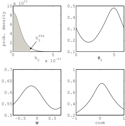
An example of the posterior pdfs for the four un-known pulsar parameters of PSR J0024−7204C (each marginalised over the three other parameters) is shown in Fig. 2. The pdfs in Fig. 2 are from the joint analysis

0 5

x 10−24 0

2 4 6 8 10x 10

23

h 0

prob. density

−0.5 0 0.5

0.5 0.55 0.6 0.65 0.7

ψ

−1 0 1

0.2 0.4 0.6 0.8 1

cosι

0 5

0.1 0.2 0.3 0.4 0.5

φ₀

h 0 95%

FIG. 2: The marginalised posterior pdfs for the four unknown pulsar parametersh0,φ0, cosιandψ, for PSR J0024−7204C

using the joint data from the three LIGO detectors over S3 and S4.

of the three LIGO detectors using the S3 and S4 data, all combined coherently. The shaded area in theh0

pos-terior shows the area containing 95% of the probability as given by Eq. (3.3). In this example the posterior on

h0 is peaked ath0 = 0, though any distribution that is

credibly close to zero is consistent with h0 = 0. Indeed

B. Binary models

Our previous known pulsar searches [2, 3] have ex-cluded pulsars within binary systems, despite the ma-jority of pulsars within our detector band being in such systems. To address this, we have included an additional time delay to transform from the binary system barycen-tre (BSB) to pulsar proper time, which is a stationary reference frame with respect to the pulsar. The code for this is based on the widely used radio pulsar timing soft-ware TEMPO [20]. The algorithm and its testing are discussed more thoroughly in Ref. [21].

There are five principal parameters describing a Kep-lerian orbit: the time of periastron,T0, the longitude of

periastron,ω0, the eccentricity,e, the period,Pb, and the

projected semi-major axis,x=asini. These describe the majority of orbits very well, although to fully describe the orbit of some pulsars requires additional relativistic pa-rameters. The basic transformation and binary models below are summarised by Taylor and Weisberg [17] and Lange et al. [22], and are those used in TEMPO. The transformation from SSB time tb to pulsar proper time T follows the form of Eq. (1.5) and is

tb=T+ ∆R+ ∆E+ ∆S, (3.5)

where ∆Ris the Roemer time delay giving the

propaga-tion time across the binary orbit, ∆Eis the Einstein delay

and gives gravitational redshift and time dilation correc-tions, and ∆S is the Shapiro delay and gives the general

relativistic correction (see Ref. [17] for definitions of these delays).

The majority of binary pulsars can be described by three orbital models: the Blandford-Teukolsky (BT) model, the low eccentricity (ELL1) model, and the Damour-Deruelle (DD) model (see Refs. [17, 20, 22] for further details of these models). These different models make different assumptions about the system and/or are specialised to account for certain system features. For ex-ample, the ELL1 model is used in cases where the eccen-tricity is very small, and therefore periastron is very hard to define, in which case the time and longitude of perias-tron will be highly correlated and have to be reparame-terised to the Laplace-Lagrange parameters [22]. When a binary pulsar’s parameters are estimated from radio ob-servations using TEMPO the different models are used accordingly. These models can be used within our search to calculate all the associated time delays and therefore correct the signal to the pulsar proper time, provided we have accurate model parameters for the pulsar.

IV. PULSAR SELECTION

The noise floor of the LIGO detectors increases rapidly below about 50 Hz, so pulsar targets were primarily se-lected on their frequency. The choice of a 50 Hz grav-itational wave frequency cut-off (pulsar spin frequency

of 25 Hz) is somewhat arbitrary, but it also loosely re-flects the split between the population of fast (millisec-ond/recycled and young) pulsars and slow pulsars.

All 154 pulsars with spin frequencies > 25 Hz were taken from the ATNF online pulsar catalogue [10] (de-scribed in Ref. [23]). The accuracy of these parameters varies for each pulsar and is dependent on the time span, density of observations and the noise level of the timing observations. Clearly it is important to ensure that pa-rameter uncertainties do not lead to unacceptable phase errors in the heterodyne. Pulsars are not perfect clocks, so the epoch of the parameters is also important as more recent measurements will better reflect the current state of the pulsar. Importantly, there is near-continuous mon-itoring of the Crab pulsar at Jodrell Bank Observatory, and as such its parameters are continuously updated [24]. Precise knowledge of the phase evolution of each target pulsar is vital for our analysis, and possible effects that may lead to a departure from the simple second-order Taylor expansion are discussed below.

A. Pulsar timing

Using TEMPO, we obtained the parameters of 75 pul-sars from the regular observation programs carried out at Jodrell Bank Observatory and the Parkes Telescope (see Ref. [25] for details of the techniques used for this). For 37 of these the timings spanned the period of S3. These same model parameters were used to extrapolate the pulsar phases to the period of S4. The effect of pa-rameter uncertainties on this extrapolation is discussed in§IV B, but is only important in its effect on the extrap-olated phase. For those pulsars observed during S3 the interpolation is taken to be free from significant error.

The parameters for 16 additional pulsars (for which new timings were not available) were taken directly from the ATNF catalogue, selected using criteria described in the following section. The parameters of the X-ray pulsar PSR J0537−6910 were taken from Ref. [26] and those for the Crab pulsar from the Jodrell Bank monthly ephemeris [24]. The remaining 61 pulsars (from the orig-inal list of 154) were not timed with sufficient confidence and were excluded from the search. This included many of the newly discovered pulsars (for example the 21 mil-lisecond pulsars in the Terzan 5 globular cluster [27]) for which accurate timing solutions have yet to be published. We therefore had a catalogue of 93 timed pulsars for our gravitational wave search.

B. Error propagation in source parameters

with all the binary orbital parameters. Some of these uncertainties are correlated, for example the error on fre-quency could affect the accuracy of the first frefre-quency derivative, and the binary time of periastron and longi-tude of periastron are also highly correlated.

We took a ‘worst-case scenario’ approach by adding and subtracting the quoted uncertainties from the best-fit values of all the parameters to determine the com-bination which gave a maximum phase deviation, when propagated over the period of the run (either S3 or S4), from the best fit phase value calculated over the same time period. For example if we assume φ(tS3) given by

Eq. (1.3) (ignoring for simplicity the φ0 and ¨ν terms)

is the best fit phase over the time span of S3, tS3, the

maximum phase uncertainty is

∆φerr = max

h

φ(tS3)±2π n

(ν±σν)(tS3±σtS3

+1

2( ˙ν±σν˙)(tS3±σtS3)

2_{+. . .}o i

, (4.1)

where theσs are the uncertainties on the individual pa-rameters. Correlations between the parameters mean that this represents an upper limit to the maximum phase uncertainty, sometimes greatly overestimating its true value.

There are 12 pulsars with overall phase uncertainty

> 30◦ _{in S3, which we take as the threshold of} ac-ceptability. A 30◦ _{phase drift could possibly give a} factor of ∼ 1 − cos 30◦ _{= 0.13 in loss of} sensitiv-ity for a signal. Nine of these are in binary sys-tems (PSRs J0024−7204H, J0407+1607, J0437−4715, J1420−5625, J1518+0205B, J1709+2313, J1732−5049, J1740−5340 and J1918−0642) and in five of theseT0and

ω0 contribute most to the phase uncertainty. For the

three isolated pulsars (PSRs J0030+0451, J0537−6910, and J1721−2457) the phase error is dominated by uncer-tainties in frequency and/or position.

Applying the same criterion to the time-span of S4 we find that PSR J1730−2304 rises above the limit. For this pulsar its parameter uncertainties do not affect it for the S3 analysis as it was timed over this period, how-ever when extrapolating over the time of the S4 run the uncertainties become non-negligible.

In total there are 13 pulsars rejected over the combined run. This highly conservative parameter check reduces our 93 candidate pulsars to 80.

C. Timing noise

Pulsars are generally very stable rotators, but there are phenomena which can cause deviations in this stabil-ity, generically known as timing noise. The existence of timing noise has been clear since the early days of pul-sar astronomy and appears as a random walk in phase, frequency or frequency derivative of the pulsar about the regular spin-down model given in Eq. (1.3) [28]. The strength of this effect was quantified in Ref. [28] as an

activity parameter A, referenced to that of the Crab pul-sar, and in Ref. [29] as a stability parameter ∆8. A is

based on the logarithm of the ratio of the rms residual phase of the pulsar, after removal of the timing model, to that of the Crab pulsar over an approximately three-year period. ∆8 is not based on the stochastic nature of the

Crab pulsar’s timing noise and and is defined for a fixed time (108_{s) as}

∆8= log

₁

6ν|ν| ר (10

8_s)3

. (4.2)

This assumes that the measured value of ¨ν is dominated by the timing noise rather than the pulsar’s intrinsic second spin-down derivative. Although generally true, this assumption is not valid for the Crab pulsar and PSR J0537−6910, where a non-timing noise dominated ¨

ν can be measured between glitches3_{. This quantity}

re-lates to the pulsar clock error caused by timing noise. The value of ¨ν is so small as to be unmeasurable for most pulsars, although an upper limit can often be de-fined. Arzoumanianet al. [29] deduce, by eye, a linear relationship between ∆8 and log ˙P of

∆8= 6.6 + 0.6 log ˙P , (4.3)

where ˙P =−ν/ν˙ 2 _{is the period derivative.}

As defined, ∆8is a somewhat imprecise indicator of the

timing noise, not least because the time span of 108

sec-onds chosen by Arzoumanianet al. was simply the length of their data set. A preferred measure may simply be the magnitude and sign of ¨P, but we shall continue to use the ∆8parameter as our timing noise magnitude estimate for

the current analysis. A thorough study of timing noise, comparing and contrasting the various measures used, will be given in Ref. [30] (also see Refs. [25, 31]).

There is a definite correlation between the ∆8

param-eters, spin-down rate and age. Young pulsars, like the Crab pulsar, generally show the most timing noise. The categorisation of the type of timing noise (i.e., phase, fre-quency or frefre-quency derivative) in Ref. [28] allowed them to ascribe different processes for each. The majority of pulsars studied showed frequency-type noise, possibly a result of random fluctuations in the star’s moment of in-ertia. The actual mechanism behind the process is still unknown, with Cordes and Greenstein [32] positing and then ruling out several mechanisms inconsistent with ob-servations.

Timing noise intrinsically linked to motions of the elec-tromagnetic emission source or fluctuations in the mag-netosphere, rather than the rotation of the pulsar, is im-portant in the search for gravitational waves as it may allow the relative phase of the electromagnetic and gravi-tational signals to drift. The implications of timing noise

3_{These two pulsars are among the most prolific glitchers, and in}

any global fit to their parameters the value of ¨νwould most likely

in this context are discussed by Jones [33]. He gives three categories of timing noise, not necessarily related to the three types of timing noise given by Cordes and Helfand [28], having different effects on any search. If all parts of the neutron star are strongly coupled on short timescales, there should be no difference between the electromag-netic phase and gravitational wave phase. If the tim-ing noise were purely a magnetospheric fluctuation then phase wandering caused by timing noise would not be seen in the gravitational wave emission. The third possi-bility, whereby the electromagnetic emission source wan-ders with respect to the mass quadrupole, could result from a weak exchange of angular momentum between the parts of the star responsible for electromagnetic and gravitational wave emission. Jones describes the ratio of the electromagnetic and gravitational timing noise phase residuals (∆Φ) by a parameter α= ∆Φgw/∆Φem, with

the three types of timing noise described above corre-sponding toα= 1, 0 and−Iem/Igw respectively, where

theIs represent the moments of inertia of the electromag-netic and gravitational wave producing components. In principle this factor could be included as another search parameter. However, given the cost of including an extra parameter in this search, and given that it is plausible that that all parts of a neutron star are tightly coupled on the timescales of interest here, we will assume rigid coupling between the two components, i.e set α = 1, corresponding to the gravitational and electromagnetic signals remaining perfectly in phase.

The Crab pulsar is regularly monitored [24] on timescales that are sufficiently short to allow its timing noise to be effectively removed using a second heterodyne procedure [34]. Like the Crab pulsar, PSR J0537−6910 is young, has a high glitch rate and also shows high levels of timing noise [26]. Unfortunately, unlike the Crab pulsar, we have no regular ephemeris for it that covers our data set, and timing irregularities are likely to be too great for historical data to be of use. We therefore have excluded PSR J0537−6910 from the analysis. For less noisy pulsars we still need a method of estimating the effect of timing noise on phase evolution that does not rely on continu-ous observation. One such estimate is the ∆8 parameter

given by Eq. (4.2), which can provide a measure of the cu-mulative phase error. For those pulsars with a measured ¨

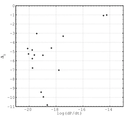
ν we use this estimate to obtain a corresponding value of ∆8 as shown in Fig. 3. This should provide a reasonable

estimate of the timing noise over the timespan of the pul-sar observation. Again we apply our criterion that cumu-lative phase errors of>30◦ are unacceptable. In Fig. 3 there are four pulsars (those with the four largest ∆8

values), with measured ¨ν, for which this is the case, and therefore timing noise could be a problem (having already noted the Crab pulsar and PSR J0537−6910 as excep-tions): PSRs J1748−2446A, J1823−3021A, J1913+1011, and J1952+3252. For pulsars with no measured ¨ν we use the approximate linear relation between the period derivative ˙P and ∆8 given in Eq. (4.3). The low ˙P

val-ues for these pulsars implies that timing noise will be

−20 −18 −16 −14

−11 −10 −9 −8 −7 −6 −5 −4 −3 −2 −1 0

log(dP/dt) ∆8

FIG. 3: The values of ∆8 for our selection of pulsars with

measured ¨ν.

negligible.

In addition to the above, there are some pulsars in globular clusters for which there is no ¨ν and for which

˙

P is negative ( ˙ν is positive), so no value of ∆8 can be

assigned either through Eqs. (4.2) or (4.3). For these pulsars the value of ˙ν (and therefore ¨ν) must be rather small to have been affected by motions within the cluster (discussed more in§VI), so timing noise should again be negligible.

For pulsars which were re-timed over the period of S3 timing noise will be negligible (for the S3 analysis at least) as any timing noise, which usually has variations on time-scales of several months to years, will have been ab-sorbed in the parameter estimation. PSRs J1748−2446A and J1823−3021A were re-timed over S3 meaning that their S3 results will stand, although the other two will not. However, being conservative we will remove all four pulsars with large values of ∆8, and PSR J0537−6910, in

which timing noise could be problematic, from the S4 and joint analysis. Note that PSR J0537−6910 is vetoed by both the parameter error criterion and our timing noise criterion.

This reduces our final number of well parameterised pulsar targets to 78 for the S3 analysis and 76 for the S4 and joint analyses. The 76 pulsars include 21 of the 28 from the previous study of Abbott et al. [3], and so through our selection criterion we lose the fol-lowing 7 previously analysed pulsars: PSRs J0030+0451, J1721−2457, J1730−2304, J1823−3021A, J1910−5959B, J1913+1011, and J1952+3252. The same selection rules were not applied over S2, especially of note was that no timing noise criterion was considered, which accounts for three of the pulsars we lose between the two analyses. Also our 30◦ _{rule was strictly applied, which the other} four pulsars just exceeded.

pulsars mentioned above, however the various parameter uncertainties preclude us setting upper limits on a total of 15 of these.

V. HARDWARE INJECTIONS

For analysis validation purposes simulated gravita-tional wave signals for a variety of sources (bursts, pul-sars, inspirals and stochastic) have been mechanically in-jected into the LIGO interferometers during science runs. During S2 two pulsar signals were injected [3]. This was increased to 10 injections in the LIGO instruments for S3 and 12 for S4 covering a wider range of signal param-eters. Extracting and understanding these injections has been invaluable in validating the analysis.

The hardware injection signals are produced using soft-ware (under LALApps [35]), which was largely developed independently of the extraction code. However, the codes do share the same solar system barycentring and detec-tor antenna response function routines, both of which have been extensively checked against other sources (e.g. checks against TEMPO in Refs. [1, 21]).

The signals were added into each of the three LIGO detectors via the position control signal going to the end test mass in one arm. Control signals in the digital servos that maintain optical cavities on resonance were summed with fake pulsar waveforms, modulating mirror positions to mimic the effect of a real spinning compact object (i.e. differential length motions with frequency and am-plitude modulations appropriate for a given sky position, frequency and spin-down). Furthermore, as the digital fake waveforms have to be converted to analog coil cur-rents of suspended optics, the injected waveforms have to be divided by the transfer function of the output chain (predominantly the pendulum), in order to produce the desired differential length response of the cavity.

The extraction of these injections is described in detail in Appendix A. They show the relative phase consistency between the detectors over the course of a run. This means that a joint analysis combining the data from all detectors is valid. The injection plots (see Figs. 7 and 8) show what we would expect our posterior plots to look like given a detection i.e. strongly peaked pdfs with very small probability at h0 = 0, as compared to those in

Fig. 2 whereh0 peaks at zero.

VI. RESULTS

A. Upper limits

Here we present 95% degree-of-belief upper limits on the amplitude of gravitational waves (h0) from the 78

pulsars identified above. The value ofh0 is independent

of any assumptions about the neutron star other than it is emitting gravitational waves at twice its rotation frequency. The results will also be presented in terms

of the pulsars’ equatorial ellipticity ε, which under the assumption of triaxiality is related toh0via Eq. (1.1) by

ε= 0.237

_h

0

10−24

r

1 kpc

1 Hz

ν

2₁₀38_{kg m}2

Izz

.

(6.1) To obtain an upper limit onεfrom that forh0we assume

a fiducial moment of inertia value of Izz = 1038kg m2.

We discuss below in Sec. VI B the effect of relaxing this assumption. Pulsar distances are taken from the ATNF catalogue [10] and are generally derived from the radio dispersion measures, with errors estimated to be of or-der 20%, although in some cases even this can be an underestimate. A critical review of pulsar distance mea-surements can be found in Ref. [36].

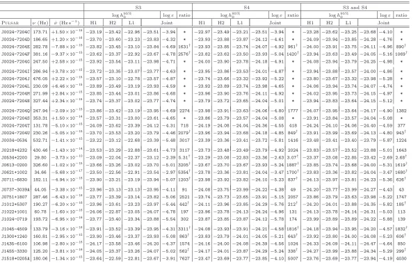
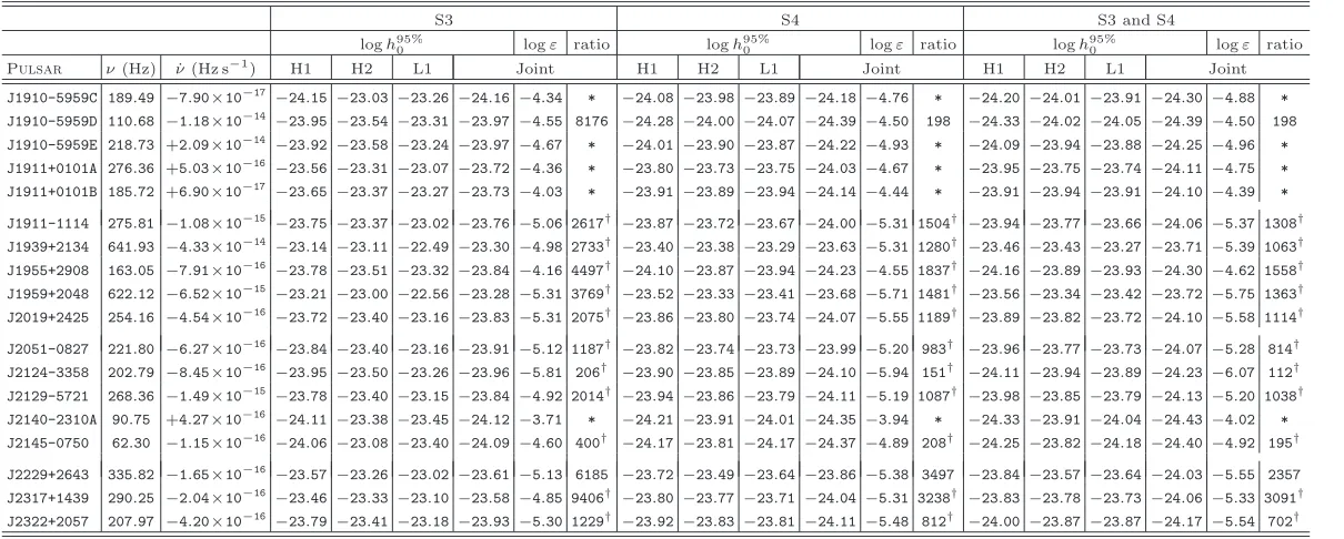
All upper limit results from the individual S3 and S4 runs along with results from the combined run, with and without GEO 600 included, are given in Appendix B in Tables III and IV. The GEO 600 data only provides comparable sensitivities to LIGO at frequencies greater than 1000 Hz, and are therefore only used in the search for PSR J1939+2134 (at the time the fastest known mil-lisecond pulsar) in S3, and additionally PSR J1843−1113 in S4 and the combined run. Inclusion of GEO 600 does not significantly change the joint upper limits for these pulsars. For the majority of pulsars the lowest up-per limits come from the combined S3/S4 data set, al-though for 7 pulsars (PSRs J0024−7204I, J0024−7204S, J0024−7204U, J1045−4509, J1802−2124, J1910−5959D and J1911+0101B) the S4 results alone provide a lower limit. The combined S3 and S4 run results are presented in histogram form in Fig. 4. Fig. 5 shows the results compared to a joint LIGO S4 upper limit estimate curve, taken as the best sensitivity during S4. The joint upper limit sensitivity curve for the three detectors can be esti-mated by combining the detector one-sided power spec-tral densities (PSDs) via

S(f) =

Tobs H1

Sh(f)H1

+ Tobs H2

Sh(f)H2

+ Tobs L1

Sh(f)L1

−1 ,(6.2)

h95%0 = 10.8

p S(f),

whereSh(f) is the PSD and Tobs is each detector’s live

time (using the associated duty factor of each interferom-eter during the run). The factor of 10.8 is given in Ref. [1] and was calculated through simulations with Gaussian noise4_.

The results are also compared to the upper limit de-duced from the observed spin-down via Eq. (1.2) making the assumption that all rotational energy is lost through

4_{In Ref. [3] a similar plot to Fig. 5 is shown for the S2 data using}

−24.50 −24 −23.5 2

4 6 8 10 12 14

log 10(h0)

no. of pulsars

−6 −4 −2

0 2 4 6 8 10 12 14

log 10(ε)

0 2 4

0 2 4 6 8 10 12

log

10 (spin−down ratio)

FIG. 4: Histograms of the log of amplitude, ellipticity, and ratio of spin-down to gravitational wave upper limits for the combined LIGO S3 and S4 run.

102 103

10−26

10−25

10−24

10−23

10−22

frequency (Hz)

h0

Joint sensitivity over S3 and S4 Joint design sensitivity for 1 year spin−down ULs

Joint ULs

FIG. 5: The combined S3 and S4 upper limit results on the amplitude of gravitational waves for 76 pulsars using LIGO data compared to the joint sensitivity curve.

gravitational wave emission. The spin-down limit is seen as a natural crossing point after which gravitational-wave data, including upper limits, have a likely bear-ing on the nature of the neutron star. The spin-down upper limit will obviously depend on ˙ν. This value how-ever, can be masked by radial and transverse motions of the object (see Ref. [37] for discussion of these ef-fects). The Shklovskii effect [38], in which the pulsar has a large transverse velocityv, will cause an apparent rate of change in the pulsar’s period of

˙

PS=

v2

rcP. (6.3)

Its 1/r dependence makes this effect more prominent for nearby pulsars. In the ATNF catalogue [10] values of the

intrinsic period derivative ˙Pint = ˙P−P˙Scan be obtained

where this effect has been corrected for. This provides a measure of intrinsic (rather than apparent) spin-down5

and, when available, is used in the spin-down ratio re-sults.

The observed value of ˙Pobs will also differ from its

in-trinsic value, ˙Pint, if the pulsar is accelerating – a likely

scenario in the gravitational field of a globular cluster [37]. Any line-of-sight component to the acceleration,

a||, will give an observed value of

˙

Pobs= ˙Pint+

a||

c P (6.4)

whereP is the spin period [39]. These effects can cause pulsars to have apparent spin-ups (seen in quite a large number of globular cluster pulsars) although are only strong enough to greatly affect pulsars with intrinsically small period derivatives. There are still many globular clusters for which the radial accelerations have not been measured, therefore no firm spin-down upper limit can be set, making the direct gravitational wave results a unique limit.

Highlights of the combined S3/S4 results include the tightest strain upper limit set on a pulsar ofh95%

0 = 3.2×

10−25_{for PSR J1603−7207, the smallest ellipticity atε=}

8.5×10−7 _{for PSR J2124−3358, and the closest upper}

limit to the spin-down limit at a ratio of 2.7 for the Crab pulsar (PSR J0534+2200).

5_{Note that the heterodyne procedure still needs to make use of the}

B. Dependence on the moment of inertia

The pulsar ellipticity results detailed above assume a moment of inertia of 1038_{kg m}2_{, which is the standard}

fiducial number used in the literature. However, modern theoretically computed equations of state (EOS) gener-ally predict somewhat larger moments of inertia for stars more massive than 1M⊙, a group which includes all neu-tron stars with measured masses (see Ref. [40]). There-fore the dependence on moment of inertia should be con-sidered.

Bejger, Bulik, and Haensel [41] give an overview of the theoretical expectations for the moment of inertia. Their Fig. 2 plots the moment of inertia vs. mass for several theoretically predicted types of EOS. The maxi-mum moment of inertia they find (after varying the mass of the star) is 2.3 times the fiducial value, with stars of 1.4M⊙ having moments of inertia 1.2–2.0 except for one outlying type of EOS. Typically the maximum moment of inertia occurs for a neutron star mass of 1.7M⊙ or more. Recently masses greater than 1.6–1.7M⊙ with 95% confidence have been measured [27, 42] for some systems, making this reasonable to consider. More re-cently Lackey [43] found the highest moment of inertia to be 3.3×1038_{kg m}2_{for EOS G4 of Lackey, Nayyar, and}

Owen [44]. This is a relativistic mean-field EOS simi-lar to the GNH family considered by Bejger, Bulik, and Haensel [41] but contains no exotic phases of matter such as hyperons or quarks. Consequently, we consider the range of theoretically predicted moments of inertia to be approximately 1–3×1038kg m2.

There have been recent attempts to infer neutron star moments of inertia from observations. Bejger and Haensel [45, 46] derived a value for the Crab pulsar’s moment of inertia by equating the spin-down power to the observed electromagnetic luminosity and inferred ac-celeration of the nebula. However, this (extremely high) value is dominated by the assumptions about the highly uncertain mass and mass distribution of the nebula as well as the relativistic wind from the pulsar, and thus cannot yet be considered to give a reliable value. The double pulsar system J0737-3039 shows great promise for tighter measurements of the moment of inertia (and con-straints on the EOS) in the near future [41, 47, 48, 49]. However, for the moment we are left with the theoretical range quoted above.

As suggested in Ref. [50], instead of using Eq. (6.1) to set a limit onε assuming a value ofIzz, one can use

it to set a limit on the neutron star quadrupole moment

≈Izzεwithout relying on any assumption aboutIzz. The

limit on the quadrupole moment can then be used to help define an exclusion region in theI-εplane. This exclusion region allows one to read off an upper limit on ε as a function of the EOS-dependent moment of inertia. The spin-down can also be used to provide exclusion regions via the relation

Izz = 5|ν|c˙

5

512Gν5

1

ε2. (6.5)

Theoretical contributions to the exclusion regions come from predictions of the maximum moment of inertia and ellipticity. In terms of the exclusion region, our observa-tional upper limits onh0are far from contributing except

for the Crab pulsar, to which we now turn.

C. The Crab pulsar - PSR J0534+2200

Of the known radio pulsars, the Crab pulsar has of-ten been considered one of the most promising sources of gravitational waves. This is due to its youth and large down rate, leading to a relatively large spin-down upper limit several orders of magnitude higher than for most other pulsars. The high rate of glitching in the pulsar also provides possible evidence of asymmetry. One glitch model favoured for the Crab pulsar involves a change in the pulsar ellipticity, and breaking of the crust, as the star settles to its new equilibrium state as it spins down [37]. In the 1970s, estimates of gravitational wave strains were spurred on by the experimenters pro-ducing novel technologies which allowed the possibility of probing these low strains, with Zimmermann [51] pro-ducing estimates of gravitational wave strains from the Crab pulsar ranging fromh0≈2×10−25−10−29.

The first searches for gravitational waves from the Crab pulsar were carried out using specially designed resonant bar detectors, with frequencies of around 60 Hz [6]. The most recent result using such a bar was from 1993 and gave a 1σ upper limit of h0 ≤ 2×10−22 [7].

This upper limit was passed in the LIGO S2 run, which gaveh95%0 = 4.1×10−23 [3]. Using Eq. (1.2), and taking

Izz = 1038kg m2 and r = 2 kpc, gives a spin-down

up-per limit for the Crab pulsar ofh0<1.4×10−24, about

a factor of 30 below the S2 observational upper limit. However, the S2 limit on the Crab was at the time the closest approach to the spin-down limit obtained for any pulsar.

Our new results for the Crab pulsar (and the other 77 targets) are shown in Table III. The results improve by up to an order of magnitude over those from the S2 run, and the majority of this improvement was between the S2 and S3 runs. The results for the Crab pulsar over the S2, S3 and S4 runs are plotted on theI–ε plane in Fig. 6. The solid lines in Fig. 6 mark the lower bound-aries of exclusion regions on this plane using our upper limits obtained for the different runs. The dashed black line marks the lower boundary of the upper limit from spin-down as given in Eq. (6.5). The dashed horizontal grey lines give lower and upper bounds on the moment of inertia of 1–3×1038_{kg m}2_{, as given by our arguments}

in §VI B. It can be seen that our experimental results currently only beat the spin-down limit for moments of inertia at values greater than double the maximum of our theoretical range. However, over this range the ratio of the gravitational to spin-down upper limit ranges from 2.7 at the lowest value to only 1.5 at the largest value.

10−4 10−3 10−2 10−1 1037

1038 1039 1040 1041 1042

ellipticity ε Izz

kgm

2

S2 S3 S4 S3/S4 spin−down

FIG. 6: The moment of inertia–ellipticity plane for the Crab pulsar over the S2, S3 and S4 runs. The areas to the right of the solid lines are the experimentally excluded regions. The horizontal lines represent theoretical upper and lower limits on the moment of inertia as mentioned in§VI B. Theoretical upper limits on the ellipticity are much more uncertain, the highest being a few times 10−4_.

strongest possible signal because we know that much of the spin-down energy of the Crab goes into powering the nebula through electromagnetic radiation and relativistic particle winds. Thus it is interesting to ask how far we would need to beat the spin-down limit to have a chance of detecting a signal allowing for what is known about the non gravitational wave spin-down. Palomba [52] uses the observed braking index 2.51 of the Crab pulsar with a simple model of spin-down through gravitational radia-tion (braking index 5) combined with some other mecha-nism (braking index a free parameter) to place an upper limit of aboutε≤3×10−4. This is about 2.5 times lower than the spin-down limit and nearly 7 times lower than our result (forIzz = 1038kg m2).

The Crab pulsar experienced two glitches between S3 and S4, a large glitch on 6th _{September 2004 and a}

smaller glitch on 22nd _{November 2004 [24]. The effect}

of glitches on the relative phase between the electromag-netic pulse and any possible gravitational wave signal is unknown, so there is uncertainty whether the (phase-coherent) combined S3/S4 result is valid. The combined result stands, but the reader should be aware that it in-cludes the assumption of trans-glitch phase coherence.

VII. ASTROPHYSICAL INTERPRETATION

We have produced new, tight, upper limits on grav-itational wave signal strength from a large selection of known pulsars and for the Crab pulsar we are very near the fiducial limit set by spin-down arguments.

It can be seen from Table III and Fig. 4 that, for the majority of pulsars, the gravitational wave detector

up-per limits are at least one hundred times above those from the spin-down argument, so is there anything that we can take from the results in terms of astrophysics?

First we should note that spin-down limits on grav-itational wave luminosity are plausible, but model de-pendent. They assume a model for the structure of the neutron star (for instance, that it is not accreting and is rigidly rotating, in addition to assumptions about its equation of state) and they take dispersion measure dis-tance as a consistently good measure of true disdis-tance. There is some considerable uncertainty associated with all of these assumptions. In contrast our observations set direct limits on a source’s gravitational wave strain.

Secondly, for globular cluster pulsars the spin-down measured from radio timing observations is a combina-tion of the spin-down intrinsic to the pulsar and acceler-ation along the line-of-sighta|| in the cluster’s gravita-tional potential (see Eq. (6.4)). In general, the magnitude and sign of the acceleration is unknown but the intrinsic

˙

Pint>0 of millisecond pulsars is usually small and often

smaller than the extrinsic contribution. Only if ˙Pobs<0

one can be sure thata||<0. Therefore, the limits derived from our gravitational wave observations provide the only direct limits on ˙Pint which are independent from biasing

kinematic effects. These can be combined with the ob-served spin-down to provide a limit on the acceleration in the cluster, i.e.a||≥c( ˙Pobs−P˙gwlimit)/P.

Finally, it is interesting to note that our ellipticity lim-its are well into the range permitted by some models of strange quark stars or hybrid stars (ε ∼a few times 10−4−10−5) and are reaching into the range permitted by more conventional neutron star EOSs (ε∼a few times 10−7_{) [53].}

Currently the fifth LSC science run (S5) is underway, and this promises to beat the Crab pulsar spin-down limit within a few months of its start. For many other pulsars we should be able to reach amplitude upper limits of

<1×10−25_{and ellipticities of∼1×10}−7_.

Acknowledgments

Foundation.

[1] R. J. Dupuis and G. Woan, Phys. Rev. D 72, 102002 (2005).

[2] B. Abbottet al. (LIGO Scientific Collaboration), Phys. Rev. D69082004 (2004).

[3] B. Abbottet al. (LIGO Scientific Collaboration), Phys. Rev. Lett.94181103 (2005).

[4] B. Abbott et al. (LIGO Scientific Collaboration), arXiv:gr-qc/0605028 (2006).

[5] P. Jaranowski, A. Kr´olak, and B. F. Schutz, Phys. Rev. D58, 063001 (1998).

[6] H. Hirakawa, K. Tsubono and M. K. Fujimoto, Phys. Rev. D17, 1919 (1978).

[7] T. Suzuki, First Edoardo Amaldi Conference on Gravi-tational Wave Experiments, 115 (1995).

[8] J. Houghet al, Nature303, 216 (1983).

[9] M. Hereld, PhD thesis, California Institute of Technology (1983).

[10] Australia Telescope National Facility Pulsar Catalogue

http://www.atnf.csiro.au/research/pulsar/psrcat/.

[11] R. J. Dupuis, PhD Thesis, University of Glasgow (2004). [12] F. Acerneseet al, Class. Quant. Grav.22, 869 (2005). [13] T. Creighton, Class. Quant. Grav.20, 853 (2003).

[14] http://einstein.phys.uwm.edu/PartialS3Results

[15] B. Abbottet al. (LIGO Scientific Collaboration), Phys. Rev. D72102004 (2005).

[16] B. Abbott et al. (LIGO Scientific Collaboration) “All-sky LIGO search for periodic gravitational waves in the S4 data”, in preparation.

[17] J. H. Taylor and J. M. Weisberg, Astrophys. J.345, 434 (1989).

[18] J. R. Smithet al., Class. Quant. Grav.21, S1737 (2004). [19] S. Hildet al., J. Phys.: Conf. Ser.32, 66 (2006).

[20] http://pulsar.princeton.edu/tempo.

[21] M. D. Pitkin and G. Woan, in preparation (2006). [22] C. Lange et al., Mon. Not. R. Astron. Soc. 326, 274

(2001).

[23] R. N. Manchesteret al., Astron. J.129, 1993 (2005). [24] Jodrell Bank Crab Pulsar Monthly Ephemeris

http://www.jb.man.ac.uk/research/pulsar/crab.html.

[25] G. Hobbs et al., Mon. Not. R. Astron. Soc. 353, 1311 (2004).

[26] F. E. Marshallet al., Astrophys. J.603, 682 (2004). [27] S. M. Ransomet al., Science307, 892 (2005).

[28] J. M. Cordes and D. J Helfand, Astrophys. J. 239, 640 (1980).

[29] Z. Arzoumanianet al., Astrophys. J.422, 671 (1994). [30] G. Hobbs, A. G. Lyne and M. Kramer, in preparation. [31] G. Hobbs et al., Mon. Not. R. Astron. Soc. 360, 974

(2005).

[32] J. M. Cordes and G. Greenstein, Astrophys. J.245, 1060-1079 (1981).

[33] D. I. Jones, Phys. Rev. D70, 042002 (2004).

[34] M. Pitkin and G. Woan, Class. Quant. Grav., 21, 843 (2004).

[35] http://www.lsc-group.phys.uwm.edu/daswg/projects/lalapps.html.

[36] D. A. Frail and J. M. Weisberg, Astron. J.100, 743-757 (1990).

[37] A. Lyne and F. Graham-Smith, Pulsar Astronomy,

Cam-bridge University Press (1998).

[38] I. S. Shklovskii, Soviet Astronomy13, 562 (1970). [39] E. S. Phinney, ASP Conf. Ser. 50: Structure and

Dynam-ics of Globular Clusters (1993).

[40] S. E. Thorsett and D. Chakrabarty, Astrophys. J.512, 288 (1999).

[41] M. Bejger, T. Bulik and P. Haensel, Mon. Not. R. Astron. Soc.364, 635 (2005).

[42] D. J. Niceet al., Astrophys. J.634, 1242-1249 (2005). [43] B. D. Lackey, Undergraduate honours thesis, The

Penn-sylvania State University (2006).

[44] B. D. Lackey, M. Nayyar and B. J. Owen, Phys. Rev. D

73, 024021 (2006).

[45] M. Bejger and P. Haensel, Astron. Astrophys.396, 917 (2002).

[46] M. Bejger and P. Haensel, Astron. Astrophys.405, 747 (2003).

[47] I. A. Morrisonet al., Astrophys. J.617, L135 (2004). [48] J. M. Lattimer and B. F. Schutz, Astrophys. J.629, 979

(2005).

[49] M. Krameret al., Science314, 5796, 97 (2006).

[50] M. Pitkinet al.(LIGO Scientific Collaboration), Class. Quant. Grav.22, S1277 (2005).

[51] M. Zimmerman, Nature271, 527 (1978). [52] C. Palomba, Astron. Astrophys.354, 163 (2000). [53] B. Owen, Phys. Rev. Lett.95, 211101 (2005).